Time drift of cosmological redshifts and its variance
Abstract
The contribution of cosmological perturbations to the time drift of the cosmological redshift is derived. It is shown that the dominant correction arises from the local acceleration of both the emitter and the observer. The amplitude of this effect is estimated to be of the order of 1% of the drift signal at , but can easily be lowered down to 0.1% by using many absorption lines and quasars.
I Introduction
The increasing observational evidences that the expansion of the universe is accelerating (see Ref. refsn; refdata and reference therein) has stimulated a rising interest to the reconstruction of its expansion history. An important outcome of these theoretical studies is to clarify the sensitivity of observational tests to dark energy properties and to assess how each could be corrupted by extra-noise from other cosmological effects. Comprehensive investigations of these nuisances have been carried out on “standard” tests, like SNIa, weak lensing, BAO, CMB, ISW or clusters of galaxies.
In contrast, very few focussed on the time drift effect that changes the observed redshift of an object as function of time. The recent claim that it may drive the conceptual design of instrument for next generation giant telescopes raised the need that similar attention should be paid to the theoretical ground of this novel technique. Interestingly, such an observation may lead to a better understanding of the physical origin of the recent acceleration refde; refde2 and to a determination of the dark energy equation of states Lake07 as well as constraints on dark energy models demodels or tests of the variation of fundamental constants constant; Molaro.
As first pointed out by Sandage Sandage, in a homogeneous and isotropic spacetime, the time drift of the observed redshift is directly related to the Hubble function by
| (1) |
Given the most likely ranges of cosmological parameter values derived from observations, in a CDM model the typical amplitude of the redshift drift is of order on a time scale of yr, for a source at redshift . This corresponds to a spectroscopic tiny velocity shift, , of . Fig. 1 (left panel) shows the time drift as function of redshift for the standard CDM model and a dark energy models with an equation of state changed by only 10% (), all other parameters being kept constant. Both curves have similar shape but the difference the drifts between a standard CDM model and cosmological models tends to zero at hight redshift. Fig. 1 (right panel) depicts this difference for two models with either or .
The feasibility of this measurement is most challenging and impossible with present-day astronomical facilities. However, it was recently revisited Loeb in the context of the new generation of Extremely Large Telescopes11 1 http://www.eso.org/projects/e-elt/Publications/ ELT_SWG_apr30_1.pdf (ELT), arguing that with such outstanding collecting areas one could measure velocity shifts of order over a 10 year period from the observation of the Lyman-alpha forest on QSO absorption spectra. In particular, it is one of the main science driver to design the COsmic Dynamics EXperiment (CODEX) spectrograph Pasquini1; Pasquini2 for the future European ELT (E-ELT).
The performances of CODEX and its capability to measure a time drift of very distant objects were estimated using Monte-Carlo simulations of quasar absorption spectra. The expected velocity accuracy of this experiment can be written as follows (see Ref. Pasquini1)
provided the absorption lines are resolved. denotes the signal-to-noise ratio, for a pixel scale of and is the number of quasars. Thus, spectroscopic measurements of about 40 quasars with ten years apart can reach a accuracy. This is within the reach of a CODEX instrument mounted on a meter ELT by observing a 16.5th magnitude QSO during 2000 hrs Pasquini1.
Many systematic effects that may spoil the time drift signal, such as Earth rotation, proper motion of the source, relativistic corrections etc., are discussed in Ref. Pasquini1. The acceleration of the Sun in the Galaxy seems more a serious problem because its amplitude may be of the same order than the cosmic signal. However, it has not been measured yet, so its nuisance is still unknown. On the other hand, subtle contaminations like accelerations produced by large scale structures have never been estimated in the error budget. The purpose of this work is to address this issue and to estimate whether it may hamper the cosmological interpretation of the time drift.
II Cosmological perturbations
Eq. (1) relates the time drift of the observed redshift to the Hubble function, assuming a perfectly homogeneous and isotropic Friedmann-Lemaître spacetime. In the real universe, however, velocity terms arising from cosmological perturbations add up as noise contributions and increase the scatter of the redshift drift around its mean value.
The distribution of the redshift drift can be predicted using the expression of to first order in the cosmological perturbations. It is derived in the Appendix A of this work. At first order in the metric perturbations and in it writes
| (2) |
with
| (3) |
This formula involves both Bardeen potentials, and , and the peculiar acceleration, . A dot denotes a derivative with respect to observer proper time and is the direction of observation. and refer to the observer and emitter respectively (see the Appendix more precise definitions of all the variables involved in this equation).
The first term at the right hand side of Eq. (3) clearly arises from the local position of the observer. The second term of Eq. (3) encodes Doppler effect due to the relative motion of the observer and the source as well as the equivalent of the integrated Sachs-Wolfe term SW; pubook. Eq. (3) is the analog of the (direction dependent) temperature anisotropy of the cosmic microwave background (CMB) compared to the mean CMB temperature.
III Estimate of the variance
The variance of can be split into contributions coming from the time dependence of the gravitational potentials, , and from the peculiar acceleration, .
The estimation of demands a full description of the time evolution of the potential, both at emission and observing times. In the following we derive it and discuss its properties using the linear cosmological perturbation theory. The validity of this approach will be more thoroughly addressed in the next section.
Using the linear theory of structure growth, the density contrast can be split as , where comprises all details on the initial conditions. The growth rate is the growing solution of the equation
| (4) |
where is the time dependent reduced density parameter for the gravitating matter (see ref. revue for details). On sub-Hubble scales, Einstein equations imply that and .
As the redshift increases, the dynamics of the universe is closer and closer to the one an Einstein-de Sitter Universe. is therefore almost constant and is expected to vanish. This is no longer true at low redshift, when the cosmological constant (or the spatial curvature) starts to dominate. Instead, the time evolution of the potential writes
| (5) |
where comprises the intrinsic evolution of the potential produced by the growing perturbations. In a flat CDM, is explicitly given by
| (6) |
where and where is a hypergeometric function.
Using Eq. (5) it is then easy to express the r.m.s. of from the r.m.s. of the mass density fluctuations, , as derived from the Poisson equation. More precisely
| (7) |
where is the power spectrum of the density contrast, , and are the Fourier modes of . To estimate , we adopt the prescription by Bond et al. bbks for the transfer function and the normalization . The redshift dependence of the power spectrum is then the one of the growing mode, , normalized to unity at .
Turning to the gravitational potential, it appears that, in the standard model of cosmology with a primordial spectrum of index , the amplitude of the potential fluctuations is IR divergent. However, since the previous calculation is only valid for sub-horizon modes, it is necessary to introduce a cut-off for modes typically beyond the Hubble scale. The expected potential fluctuations then drop to more realistic amplitudes of . It follows that, for a source at redshift , the r.m.s. of induced by the time variation of the gravitational potential is
| (8) |
which is of order , a
small number indeed.

The contribution of the peculiar acceleration, , is less obvious to derive because we do not have a complete theory that describes the expected distribution of the local line-of-sight acceleration. However, in the cosmological linear theory not only are the metric components supposed to be small (as explicitly used above), but also the density contrast and the velocity gradients (compared respectively to unity and ), see Ref. revue.
The Lyman-alpha forest is believed to be dominated by low density clouds of intergalactic medium, with individual accelerations primarily triggered by large-scale structures. Assuming then linear theory holds in our context, the local acceleration writes , so that
| (9) |
In terms of the dimensionless divergence , the linear continuity equation reduces to at linear order. This implies that the Fourier components of the velocity, density contrast and potential are related by and . Using our previous estimate of , one easily derives the r.m.s. of the two contributions to ,
| (10) |
that depends on the emission time only through the factor , and
| (11) |
where .
These two terms are independent and should be summed quadratically. The resulting r.m.s. of depicted on Fig. 1 (right panel) shows is the dominant contribution at all redshifts. It rises to a percent level from to . At , , while is ten times smaller. Both terms have similar behaviour and are basically unchanged for any realistic flat cosmology having and effective close to , but note that this is a priori not the case for any model.
IV Discussion
Assuming the cosmological time drift derived from QSO absorption lines by the Lyman-alpha forest may be contaminated by extra-acceleration of clouds by massive structures, it is legitimate to question the validity of the linear regime approximation used throughout this work.
Let us first consider the acceleration of an absorbing Lyman-alpha
cloud. On large scales, clouds are located inside filaments
infalling towards massive clusters or super-clusters of galaxies.
Assume, then, the acceleration is due to the gravitational
attraction of a super-cluster with typical mass of order
, localized at 10 Mpc from the cloud. The
Newtonian acceleration is about . In comparison, the
Hubble acceleration is so that . This ratio may change by one
order of magnitude, depending on the mass and length scales one
may consider for clusters, super-clusters or filaments, but is
always sufficiently small to keep the linear approximation valid.
It is also worth noticing its amplitude is close to theoretical
expectations derived in the previous Section. We therefore
speculate the simple interpretation of our theoretical estimate as
being primarily due to the acceleration of the nearest rich
cluster is pertinent22
2
Liske et al. (in preparation)
also estimated the contamination of the drift signal produced by
peculiar motions. In contrast to our analysis done in a full
General Relativity context, they simply used Special Relativity
formalism. Note that peculaccel derived the peculiar
acceleration of strong gravitational potentials like clusters of
galaxies but to predict the peculiar velocity drift over several
decades produced by nearby systems on a test particle. Both
results agree with our predictions.. To confirm this and get more
sophisticated description of accelerations the
use of numerical simulations is indeed necessary.
In practice, a time drift is not measured from a single absorption line but by averaging several lines spread over a spectral range defined by the spectrograph. If the acceleration of Lyman-alpha clouds is primarily driven by clusters of galaxies located around their neighborhood, then clouds are not dynamically independent and accelerations of closeby clouds are correlated. We are thus interested in the variance of , averaged over a bound comoving distance along the line of sight,
It is related to the variance from correlations obtained on a single line by
where the coefficient depends on the physical size over which the average is performed. is the redshift range explored by the spectrograph at the mean redshift : . For a CDM universe, it corresponds to a comoving distance of , with Mpc. can be computed from the correlation of the acceleration field,
as
| (12) |
where is the size of the comoving radial distance over which the average is performed.
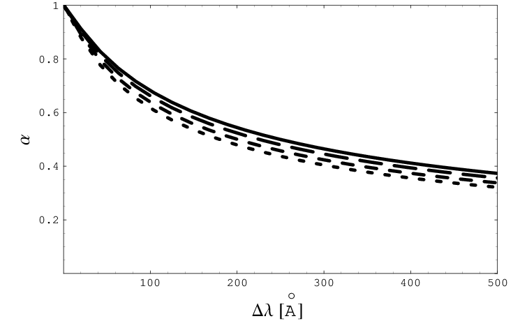
If we could naively split the Lyman-alpha forest along a line if sight into radial bunches of physically decoupled cloud systems, without correlated accelerations, would provide an estimate of the number of bunches. From an observational point of view, expresses the effective number of absorption line systems without correlated acceleration probed by a spectrograph covering a wavelength range around the mean redshift . It increases when the spectral coverage of the spectrograph increases (see Fig. 2). For example, if , and , that is (see Fig. 2) respectively, then is 0.69, 0.55, and 0.38, and 2.1, 3.3 and 6.9. However, only takes into account one light of sight. If we average over randomly selected lines of sight, then we expect that
| (13) |
Hence, the spectral range of the spectrograph together with the number of lines of sight can easily drop the contribution of cosmological perturbation to the variance budget below a level.
It is interesting to notice that the theoretical values of derived in the previous paragraph can easily be interpreted and predicted from simple physical arguments. The spectral range of a CODEX-like spectrograph as described in Ref. Pasquini1, is . At a redshift of , it corresponds to and to a comoving length of Mpc. If we assume that the coherence scale of the velocity field is the typical size of the super-cluster (30 Mpc), then CODEX can probe about 10 independent systems per line of sight. This is of the same order as for discussed above, which confirms its interpretation as an effective number of uncorrelated cloud systems. It also simply explains why , which is nothing but the inverse square root of this number.
V Conclusion
In order to measure the cosmological time drift of the redshift, many systematic effects will have to be understood. Besides the systematic errors of astrophysical origin that may affect the observation of the Lyman-alpha forest, large scale structures will induce a dispersion of . This work addresses this issue.
First, we have derived the expression of the time drift of cosmological redshift at first order in the perturbation. This was then used to estimate its variance and then to demonstrate it depends on two main effects, the accelerations and the local gravitational potential at both the source and observer positions.
The contributions at the observer position have not been discussed further. High precision astrometric observations with GAIA will soon provide exquisite knowledge of the motion of the Earth in the Milky Way. It will pinpoint all local acceleration terms with enough accuracy to remove this contribution easily gaiaref.
In contrast, the contributions at the source position are much more difficult to subtract. In the linear regime, we have shown that the gravitational potential contribution is negligible while the acceleration of the source is typically of the order of 1% at . We argue a dominant contribution to this term is the acceleration of galaxy clusters near the source.
In order to understand whether the amplitude of this variance can be reduced, we have estimated the effect of averaging the signal over several absorption lines. One can either profit from the total spectral range covered by the spectrograph to measure the drift from all lines detected along a line of sight, provided correlated acceleration contributions are taken into account, or use the mean drift over many randomly selected lines of sight. The first option reduces the variance by the square root of the number of uncorrelated clouds systems along a line of sight, the second by the square root of the number of independent lines of sight. For an instrument having the current specifications of the CODEX spectrograph, it is then easy to drop the contribution of large-scale structures to the total variance of the time drift down to a 0.1% level.
Acknowledgements: We thank Jochen Liske and Luca Pasquini for providing Ref. Pasquini1 before publication and for their comments, Patrick Petitjean for useful discussions, and Eric Linder his useful comments. We also thank Stéphane Charlot and Jean-Gabriel Cuby for organizing the Programme National de Cosmologie discussion on ELT which triggered these questions.
References
- (1)
A. Riess et al., Astrophys. J. 607 (2004) 665;
P. Astier et al., Astron. Astrophys. 447 (2006) 31. - (2)
D. Spergel et al., Astrophys. J. Supp. 148 (2004)
175;
D. Eisenstein et al., Astrophys. J. 633 (2005) 560. - (3) J.-P. Uzan, Gen. Relat. Grav. 39 (2007) 307, [astro-ph/0605313].
- (4) B. Ratra and P.J.E. Peebles, Rev. Mod. Phys. 75 (2003) 559.
- (5) K. Lake, [astro-ph/0703810].
- (6)
P.-S. Corasaniti, D. Huterer, and A. Melchiorri,
Phys. Rev. D 75 (2007) 062001;
A. Balbi and C. Quercellini, [arXiv:0704.235];
H. Zhang, W. Zhong, and Z.-H. Zhu, [arXiv:0705.4409]. - (7)
J.-P. Uzan,
Rev. Mod. Phys. 75 (2003) 403;
J.-P. Uzan, [astro-ph/0409424]. - (8) P. Molaro et al., Proc. IAU Symposium 198 (2005) 1, [astro-ph/0601264].
- (9) A. Sandage, Astrophys. J. 136 (1962), 319.
- (10) A. Loeb, Astrophys. J. 499 (1998), L111.
- (11)
Liske et al 2008 (in preparation);
L. Pasquini et al., The Messenger 122 (2005) 10. - (12) L. Pasquini et al., Proc. IAU Symposium 232 (2005) 193.
- (13) L. Amendola, A. Balbi and C. Quercellini, [arXiv:0708.1132].
- (14) R.K. Sachs and A.M. Wolfe, Astrophys. J. 147 (1967) 73.
- (15)
P. Peter and J.-P. Uzan,
Cosmologie primordiale,
Belin (Paris, France, 2005);
F. Bernardeau, Cosmologie, CNRS Editions (Paris, France, 2007). - (16) F. Bernardeau et al., Phys. Rep. 367 (2002) 1.
- (17) J.M. Bardeen et al., Astrophys. J. 304 (1986) 15.
- (18) J.-P. Uzan and F. Bernardeau, Phys. Rev. D 63 (2001) 023004.
- (19) http://www.rssd.esa.int/SA-general/Projects/ GAIA_files/LATEX2HTML/node138.html.
Appendix A Time drift at first order in the perturbation
The redshift is defined as the ratio of the wavelengths measured at the observer and the emission (galaxy) positions, both in their rest-frame. It can be expressed in terms of the tangent timelike vector to the observer (labelled ) and emitting galaxy (labelled ), , and the tangent vector to the null geodesic joining to as
| (14) |
We want to express the redshift and its time drift at first order in the perturbations around a Friedmann-Lemaître spacetime with general metric with
| (15) |
where , i.e. we chose to work in the Newtonian gauge and have neglected the effect of gravity waves.
It is clear that if is the tangent vector to a null geodesic of then is the tangent vector to a null geodesic of . Decomposing as , where is a constant, the geodesic equation reduces to (see e.g. Ref ubcorde for details)
| (16) |
where is an affine parameter along the null geodesic, and a prime refers to a derivative with respect to the conformal time.
At first order in the perturbations, the vector field is explicitly given by . We then deduce that . Thus
| (17) |
Integrating Eq. (16), one derives that . Therefore, the redshift writes
| (18) |
where we have shifted to the conformal time. This equation indeed mimics exactly the standard Sachs-Wolfe formula SW.
At the background level, the observer and emitter are comoving so that their proper time corresponds to the cosmic time. It follows that , so Eq. (18) implies , where . Shifting back to cosmic time, we get the standard expression for the time drift of a source located at redshift , that is Eq. (1).
At first order, one has to take into account the motion of the observer and the emitter, as well as the metric perturbations. This will manifest in the difference between the cosmic time and proper time.
If at the proper time , the observer was located in () and had a proper velocity , then at a proper time
- 1.
the cosmic time is , up to terms in and
- 2.
the observer has moved to so that he is located in
(19)
The null geodesic is still evaluated at the background level so that , where is the direction of observation, and the emitter is now located . This implies that
| (20) |
Thus, plugging these new positions in Eq. (18), we obtain that with
| (21) |
where a dot refers to a derivative with respect to observer proper time. This expression gives the full redshift drift at first order in the metric perturbations and in .