EFI-07-32
NSF-KITP-07-192
Bubbling Calabi-Yau geometry
from matrix models
Nick Halmagyi
Enrico Fermi Institute, University of Chicago
Chicago, IL 60637, USA
and
Takuya Okuda
Kavli Institute for Theoretical Physics, University of California
Santa Barbara, CA 93106, USA
Abstract
We study bubbling geometry in topological string theory. Specifically, we analyse Chern-Simons theory on both the 3-sphere and lens spaces in the presence of a Wilson loop of an arbitrary representation. For each three manifold, we formulate a multi-matrix model whose partition function is the Wilson loop vev and compute the spectral curve. This spectral curve is closely related to the Calabi-Yau threefold which is the gravitational dual of the Wilson loop. Namely, it is the reduction to two dimensions of the mirror to the Calabi-Yau. For lens spaces the dual geometries are new. We comment on a similar matrix model relevant for Wilson loops in AdS/CFT.
1 Introduction and summary
A useful aspect of duality between a gauge theory and a gravitational system is the emergence of spacetime through dynamics of gauge theory. Deeper understanding of emergent geometry should help us find new formulations of string theory and quantum gravity that may be used to address fundamental questions in physics.
In gauge/gravity duality, the vacuum state corresponds to a certain background spacetime, and inserted operators to excitations. The fields of gauge theory backreact significantly to the insertion of some operators. The corresponding gravitational dual is a new geometry that shares the asymptotics with the original background. A bubble of new cycles supported by flux appears, and the new spacetime is thus called the bubbling geometry. The bubbling phenomenon was originally found for local operators [1], and was generalized to Wilson loops [2, 3, 4] in AdS/CFT. It is useful to introduce a matrix model which captures the dynamics of all the relevant fields that respond to the operator insertion [7, 8]. One is able to visualize the backreaction in terms of eigenvalue distributions, which in turn encode the bubbling geometry on the gravity side.
The current work studies the topological string version of bubbling phenomena [5], which naturally extend the Gopakumar-Vafa gauge/gravity duality [6]. More specifically we consider Chern-Simons theory on or lens space with Wilson loop insertions. The Wilson loop operator is defined as
| (1.1) |
where is the gauge field and is integrated along the unknot. For we take the unknot that generates the fundamental group. The trace is evaluated in an arbitrary representation of . Throughout the paper the symbol also denotes the corresponding Young tableau, and we parametrize it as in Figure 1. Each edge length be it or , will correspond to the size of a new cycle in the bubbling geometry.
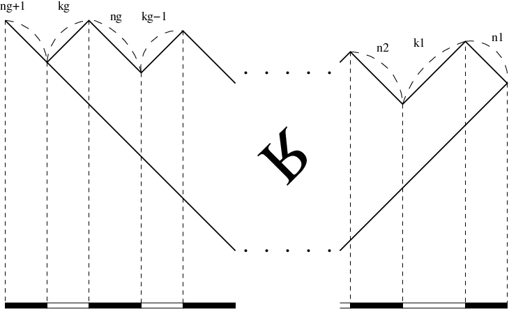
Building on the earlier work [9, 10], we formulate a matrix model whose partition function is the vev of the Wilson loop in or . We then study the eigenvalue dynamics in the large limit and derive the spectral curve. For the spectral curve is precisely the mirror of the bubbling toric Calabi-Yau geometry identified as the gravitational dual of the Wilson loop in [5]. The topology of this threefold depends on the data encoded in the Young tableau : its toric web diagram is shown in Figure 2(a)
For the lens spaces , the backreaction of the fields to the Wilson loop leads to additional classical vacua, and the path-integral splits into sectors corresponding to the different vacua. Because the matrix model we formulate computes the Wilson loop vev in each sector, we propose that for given , and , a single Wilson loop insertion is dual to a sum over bubbling geometries. Each term in the sum is the toric Calabi-Yau that is mirror to the spectral curve which we derive. The summed geometries have the same toric data shown in Figure 2(b)11 1 To take the limit in Figure 2, one need to apply an transformation. except different values of Kähler moduli. As in the case, the topology of the geometry depends on the Young tableau data.
 |
 |
| (a) | (b) |
The paper is organized as follows. Section 2 focuses on the case. In subsection 2.1 we present the matrix model for a Wilson loop in . In subsection 2.2 we derive the matrix model from physical arguments. Specifically we present it as an open string field theory of a D-brane configuration that realizes the Wilson loop. Then we algebraically derive the matrix model in subsection 2.3. In subsection 2.4, we solve the matrix model in the large limit and derive the spectral curve, which is the mirror of the bubbling Calabi-Yau found in [5].
Section 3 deals with lens space , and is structured in parallel with section 2. For each vacuum of the gauge theory with Wilson loop insertion, we derive the spectral curve. We propose that the mirror toric Calabi-Yau is the bubbling geometry dual to the Wilson loop.
Appendix A summarizes the notation regarding the Young tableau data. In appendix C we study alternative matrix models that compute the Wilson loop vev. The models are the direct analog of the matrix models for Yang-Mills considered in [11]. Appendix D is targeted at readers interested in AdS/CFT. We use the algebraic techniques in subsection 2.3 to formulate a matrix model, whose partition function is the vev of the supersymmetric circular Wilson loop in Yang-Mills. In this formulation it is very easy to derive the eigenvalue distributions for the Wilson loop found in [12, 13, 14, 11].
2 Bubbling Calabi-Yau for from a matrix model
2.1 Matrix model for a Wilson loop in
The realization that the open topological A-model can be reduced to a matrix model first appeared in Marino’s work [9], and a B-model version of this idea was subsequently derived by Dijkgraaf and Vafa [15]. Both derivations are of course mirror to each other as was demonstrated for certain examples in the nice work [10]. We are interested here in the A-model, which is of course equivalent to Chern-Simons theory [16], possibly with instanton corrections [16, 17, 18].
Marino’s observation for Chern-Simons theory on with the gauge group was that the partition function is
| (2.2) | |||||
where the topological string coupling constant is identified with the Chern-Simons coupling constant, , and is the Haar measure on with unusual integration range. On the second line we specialized to the case , and each is integrated from to . This observation by itself may not be overwhelming since it is a reformulation of Witten’s classic result for the partition function [19]. The main utility is the generalization to different manifolds, where they carry topological data [9, 10, 20, 21] and to Wilson loops which we describe in the current work.
One very interesting feature of (2.2) however is that it secretly knows about the geometric transition of Gopakumar and Vafa [6]. While Chern-Simons theory is equivalent to the open A-model on the deformed conifold, the spectral curve of (2.2) is directly related to the resolved conifold. If the Calabi-Yau threefold mirror to the resolved conifold is defined by the equation , the spectral curve is then given by . The orientifold case was worked out in [22]. Our main interest in this paper is to generalize this aspect to include the insertion of Wilson loop operators. Wilson loops in the topological gauge/gravity duality have been considered before by Ooguri and Vafa [23]. The current work and the previous work [5, 24, 25] extends this in two ways. Firstly, the full backreaction of the Wilson loop is taken into account, as explained in [24] this means the Wilson loop vev can be expressed in terms of purely closed string enumerative invariants. Secondly we provide a dictionary for a single Wilson loop in a particular representation , whereas in [23] a sum of Wilson loop insertions was considered where the summation is over representations.
Wilson loop operators
| (2.3) |
are specified by two pieces of data: the representation of the gauge group and a curve in which the gauge field is integrated over. We will be considering all representations of such that the and in Figure 1 are large and our will be the unknot.
The relation between Chern-Simons theory and the matrix model was extended to include Wilson loops in [10]:
| (2.4) |
We will show that the vev of the Wilson loop is in fact the partition function of the following matrix model:
| (2.5) | |||||
with
| (2.6) |
This is a Gaussian -matrix model with certain interactions which in the next section we explain from the target space viewpoint.
2.2 Physical derivation of the matrix model
In this subsection we derive the matrix model (2.5) as the world-volume theory in a D-brane configuration that is equivalent to the Wilson loop insertion. Further geometric transition of the branes leads to the purely closed string geometry in Figure 2(a), and the three steps are summarized in Figure 3. As we will describe, the essential details in each step can be found in the earlier work [5, 24, 25].
We start with the deformed conifold geometry given by the equation
| (2.7) |
where is the complex structure parameter that we take to be real positive. The geometry has the structure of fibration over . Let us denote the basis cycles of by and . In the base , degenerates along one line and degenerates on another. The minimal is obtained by fibering this along a line interval that connects the two loci.
We wrap branes on thus engineering the Chern-Simons theory. In addition we place a stack of branes22 2 Recall that is the number of rows in . wrapping a non-compact three cycle of topology . The cycle intersects along a circle that is identified with . These branes were introduced in [23] where the partition function obtained after integrating out the bifundamental - strings was shown to be a generating function for Wilson loop vevs. The generating function is a summation over representations of and the common to and is the defining curve of the Wilson loop. Since is non-compact one should enforce a boundary condition at infinity for the gauge field on the stack of branes which wrap . In [23] this was implicitly done by fixing the background holonomy of the gauge field along .
A different boundary condition isolates a single Wilson loop in the representation [24]. So this brane construction is equivalent to the Wilson loop insertion. See Figure 3(a). This boundary condition is equivalent to the gauge field having a nontrivial holonomy matrix along the cycle which encodes the data of .
 |
 |
 |
|---|---|---|
| (a) | (b) | (c) |
First, the above brane configuration is equivalent to another system that has a new set of non-compact D-branes, distributed along the locus where degenerates [25]. The new system has only D-branes wrapping the . As we review in Appendix B, a stack of non-compact branes sits at distance away from the for . See Figure 3(b).
Second, by considering the new ambient geometry of Figure 3(c) with more complex structure moduli given by
| (2.8) |
the non-compact branes can be compactified without changing the physics. This is a legitimate maneuver since it reduces to the deformed conifold (2.7) by making the complex structure moduli infinite and A-model depends only on Kähler moduli. The result is the D-brane system from which we can derive the matrix model (2.5).
We now have a daisy chain of Chern-Simons theories all of them on an and there are then annulus instantons which connect them [18]. The representation of the Wilson loop determines all the necessary data, in particular the -th Chern-Simons theory has gauge group , . We get annulus instantons by integrating out the massive bifundamental open strings [23]. Since the mass of the string between the -th and the -th spheres is , the interactions generated from such annulus instantons are summarized as
| (2.9) |
where is the Chern-Simons action, and is the holonomy along the unknot in the -th . Given this field theory description, we can now reduce it to a matrix model [10]:
| (2.10) |
By redefining -independent), we finally obtain (2.5). It is a nontrivial consistency check that the physical derivation here gives the values of holonomy that we need to agree with the algebraic derivation in the next subsection.
Third and finally, we can go one step further in the target space analysis though we have completed our task in this subsection, When each in Figure 3(c) undergoes a conifold transition the resulting closed string geometry is the toric Calabi-Yau manifold whose web diagram is shown in Figure 2(a). This is the Calabi-Yau manifold which is referred to as the bubbling geometry [5]. We will see in subsection 2.4 that the eigenvalue dynamics in the matrix model demonstrates the geometric transition.
2.3 Algebraic derivation of the matrix model
We now provide an algebraic derivation of (2.5). Our starting point is (2.4). Using a standard formula for the character of this can be written as
| (2.11) |
where is as usual the number of boxes in the -th row of . Now we expand this ratio of determinants into something more compatible with the matrix model:
| (2.12) | |||||
Since are dummy variables the summation over the permutation group produces identical terms, so we can write
At this point the Wilson loop insertion has been recast into a linear term in the exponential and a certain denominator term. There will be partial cancellation of this denominator term against the measure and also against the linear term. We relabel the variables as
where we recall that the Young tableau has blocks of rows. Then
The integers and are defined in Appendix A. This can be further simplified, using the trivial fact that integration variables are dummy variables, to
| (2.13) | |||||
where are defined in (2.6) and we have use the relations
| (2.14) |
At this point we essentially have an -matrix model with interactions between the matrices given by the last line in (2.13).
2.4 Spectral curve as the bubbling geometry dual to a Wilson loop in
Matrix models have an associated geometry called the spectral curve. One can think of as a single Gaussian matrix model with somewhat complicated insertion, or alternatively as we have demonstrated, as an -matrix model with certain simpler interactions. Taking the latter point of view, we now derive the spectral curve and explain its string theory interpretation.
The equations of motion for are
| (2.15) |
To solve them we define the resolvents33 3 The resolvents in another natural definition are simply related to the as .
| (2.16) |
We now assume that the eigenvalues distribute themselves into distinct cuts along the real axis, then write (2.15) an equation on the -th cut:
| (2.17) |
where and are the values of just above and below the cut, respectively. It will be convenient to rewrite this as
| (2.18) |
To derive the spectral curve, we generalize the complex analysis technique used in [26] to solve the Chern-Simons matrix model for . The crucial step in solving this model is to find a set of functions of the resolvents which are regular on the whole -plane where is of course valued. Then the asymptotics of will allow us to fix these functions exactly and finally extract the equation for the spectral curve. The technical reason that we will be able to solve this model exactly is that the interaction terms in the equation of motion can be written polynomially in terms of the resolvents. This is not the case for the related Yang Mills matrix models described in appendix D and also in [11].
We first define some new quantities
| (2.19) |
where and . Equation (2.18) implies that and are exchanged as one goes through the -th cut, leaving any symmetric polynomial of invariant under the process. The symmetric polynomial is regular on all of the cuts, and the only singularities are at . Let us now recall the definition of the -th elementary symmetric polynomials :
| (2.20) |
Together with the definition (2.16) of the resolvents, the asymptotics as determine the exactly in terms of Young tableau data:
| (2.21) | |||||
The coefficients are given by
| (2.22) |
where we introduced .
In fact the appear as the coefficients of in the expansion of the function
| (2.23) | |||||
and this vanishes upon substituting for . So we arrive at an equation for the spectral curve of the matrix model (2.5):
| (2.24) |
where are valued variables.
Since is of degree in , the spectral curve is obtained by gluing cylindrical sheets. In particular (2.24) is satisfied by the total resolvent through substitution , and the sheet on which is naturally defined has cuts. By going through the -th cut (), one moves to the -th sheet as changes to See Figure 4(a).
 |
 | |
| (a) | (b) |
This Riemann surface is related to a Calabi-Yau threefold in a way which is by now well known, namely the threefold is given by
| (2.25) |
where are valued. It is a feature of the mirror symmetry work of Hori-Vafa [27] that we can write down the toric fan directly from the Riemann surface data above. The recipe is to insert a vertex on the integral 2-dimensional lattice for each monomial appearing in (2.24). By connecting the vertices with suitable edges44 4 In the limit of large and (the large volume limit in the case, but not in the case), the difference between the GLSM algebraic coordinates [28] and our moduli is suppressed. The mirror curve of the GLSM in this limit agrees with our spectral curve including the coefficients, with the choice of internal edges in Figure 4(b) one obtains a graph, and the three-dimensional cone over this graph is the toric fan of the bubbling Calabi-Yau. The two dimensional graph is the dual graph of the toric web diagram, so from Figure 4(b) we see agreement with the previous work [5].
For concreteness we now work out the simplest case when is a rectangle. In this case the nontrivial data is
| (2.26) |
and
| (2.27) | |||||
with , and so the spectral curve is explicitly given by
| (2.28) |
2.5 Eigenvalue distribution
The exact eigenvalue distribution can be obtained by solving (2.24) for via and by computing the eigenvalue density along the cuts. Here we apply force balance to derive the approximate distribution when
| (2.29) |
Force balance is easier to understand intuitively.
We make the assumption, to be justified a posteriori, that
| (2.30) |
Because the last term in (2.15) becomes constant we have
| (2.31) |
We expect that when is large, the eigenvalues of spread over a large region, allowing us to approximate the function in (2.31) by a step function. If we order the eigenvalues so that for any , it follows that
| (2.32) |
Along the -th cut that has width , the eigenvalues of are distributed uniformly. The -th and cuts are distance apart from each other.55 5 Since is the holonomy along , its eigenvalue distribution is different from the distribution (B.63) of holonomy . In particular the eigenvalues are quantized in unit of . It should be possible to physically explain (2.32) using the fact that the matrix model captures the Wilson loop in a non-canonical framing [10]. We can thus justify the approximations above when and are all large. See Figure 5. As discussed above, this sheet is connected to other sheets through the cuts as shown in Figure 4(a).

3 Bubbling Calabi-Yau for lens space from a matrix model
3.1 Matrix model for a Wilson loop in lens space
A simple generalization of the topological A-model on is the orbifold [10]. The particular orbifold action is such that is the lens space . This space is defined by the equation
| (3.33) |
for complex variables and , together with identification
| (3.34) |
We study the Wilson loop
| (3.35) |
along a circle that is the generator of the fundamental group. We assume that the circle is the unknot.
The Chern-Simons theory on has many vacua. Since the equation of motion is solved by a flat connection, the vacua are in one-to-one correspondence with the -dimensional representations of . The group is abelian, so any such representation is a sum of one-dimensional ones. A one-dimensional representation is specified by an integer . Thus a vacuum is specified by a partition of :
| (3.36) |
Here is the number of times the -th irrep appears. The contribution of this vacuum to the partition function is given by
| (3.37) |
This matrix model was formulated in [9], and was studied for example in [10, 26, 29, 30].
According to the prescription in [10] (see also [31]), the contribution from this vacuum to the Wilson loop vev is given by
| (3.38) |
where is a vector of integers
| (3.39) |
The spectral curve for this matrix model can be derived [26] and it agrees with the string theory prediction [29].
For a large representation with large values of and , we expect a large backreaction of fields to the Wilson loop insertion. We propose that the gauge field path-integral has now more saddle points. Each saddle point specified by before insertion splits into many each of which is specified by non-negative integers satisfying the constraints
| (3.40) |
We will argue that the contribution to the Wilson loop vev from the saddle point specified by the is given by the multi-matrix model
| (3.41) | |||||
Wilson loops in the lens space matrix model have also been considered in the interesting recent work [31] and it would be of interest to apply their methods to the spectral curve in this paper.
3.2 Physical derivation of the matrix model
We now derive the matrix model from a D-brane configuration that realizes the Wilson loop in a lens space.
Let us recall that is a orbifold of the deformed conifold given by (2.7). The orbifold action is generated by
| (3.42) |
and the action on the given by (so ) defines the lens space . Since the only acts on the phases, is still a fibration of over . Let us redefine to be the 1-cycle corresponding to the generator of the fundamental group, and the 1-cycle given by the phase rotation of . We use the axes of the two cylinders (given by ) and the direction as the base . The cycle degenerates at and so does at . The cycle never degenerates.
 |
 |
 |
|---|---|---|
| (a) | (b) | (c) |
We engineer Chern-Simons theory by wrapping D-branes on the . To insert a Wilson loop along the knot , we consider D-branes that wrap the non-compact cycle in which is contractible. See Figure 6(a). The boundary condition on the branes picks out the Wilson loop insertion in representation , as explained in [5]. The boundary condition induces holonomy
| (3.43) |
along the contractible cycle . By fibering the over a semi-infinite line ending on the locus where degenerates, we obtain a 3-manifold in which is non-contractible. We can consider a configuration of D-branes wrapping this 3-manifold. Is the configuration equivalent to the one we started with, as in the case? We assume it is, and we will see evidence below. The basic nontrivial cycle in the new 3-manifold is , and the holonomy along it is given by
| (3.44) |
because is contractible. See Figure 6(b).
As in the case, it is natural to split the non-compact branes into stacks with the -th stack containing branes. We can now replace by the orbifold of the large dual geometry given by the equations (2.8). This is possible because (2.8) are invariant under the orbifold action. The non-compact branes are now replaced by compact ones wrapping copies of lens space . Thus we reach the desired system of D-branes, whose world-volume theory is copies of Chern-Simons theory on lens space , interacting via Ooguri-Vafa operators. The system is shown in Figure 6(c).
To write down the matrix model, we need to choose the vacuum of the theory. We have a Chern-Simons theory on the -th lens space. As reviewed in the previous subsection, the theory has many vacua corresponding to the choice of a flat connection. Let us choose the vacuum specified by the partition . Then according to the prescriptions in [10], the contribution to the Wilson loop vev from this vacuum is given by
| (3.45) | |||||
By redefining the variables as -independent), we obtain (3.41). It is remarkable that we get the holonomy , including the factor of , which is necessary to be consistent with the algebraic derivation. The success gives us confidence in the assumption we made above.
This brane construction makes it clear what the dual bubbling geometry should be. It should be the toric Calabi-Yau shown in Figure 2(b), where all the copies of lens space have undergone geometric transition. This proposal will be confirmed in subsection 3.4 by deriving the spectral curve of the matrix model, and showing that it is the mirror of the toric Calabi-Yau.
3.3 Algebraic derivation of the matrix model
The vector of integers in (3.37) breaks the invariance down to the product subgroup and subsequently the symmetry to . Nonetheless the Wilson loop is in the representation of and as such we cannot immediately apply all the steps we used to solve the case in section 2.3. The workaround is to consider a generating function of matrix integrals, one term of which will correspond to the Wilson loop vev . This generating function will have symmetry and thus we need only the technology used in section 2.3 to solve this case as well.
So we will consider the generating function with variables
| (3.46) | |||||
The coefficient of in (3.46) is . Since all the are dummy variables on the same footing, we can straightforwardly repeat the analysis of section 2.3 to arrive at
| (3.47) | |||||
where the eigenvalues have been divided into groups ( is again the number of groups of rows in ). To understand the coefficient of it is best to divide up the eigenvalues into and also such that
| (3.48) |
So clearly we have the constraints (3.40) and for each choice of non-negative integers which satisfies these constraints, we have the following contribution to :
| (3.49) | |||||
This is the matrix model (3.41) in the eigenvalue basis. We now solve the matrix model and derive its spectral curve.
3.4 Spectral curve as bubbling geometry for a Wilson loop in lens space
We now derive the spectral curve associated to (3.49) that captures the contribution of the particular vacuum specified by the integers . Since the gauge theory sums up such contributions, the Wilson loop is actually dual to a sum over geometries.
The equation of motion for that follows from (3.49) is
| (3.50) | |||||
and so we first define several resolvents
| (3.51) |
In terms of these we can write (3.50) as an equation on the -cut:
| (3.52) |
Following the same procedure as in section 2.4 we define some new variables66 6 Despite identical nomenclature these variables are of course unrelated to those in section 2.4.
| (3.53) |
where . Then the spectral curve is again given by (recalling once more that are valued variables)
| (3.54) |
where
| (3.55) | |||||
The difference with section 2.4 lies in the asymptotics of the elementary symmetric polynomials, from which we can determine their structure:
| (3.56) |
Some coefficients are easily determined:
where . The remaining are complex structure parameters that are determined by demanding that for the integral around the -cut. We can again write down the toric fan of the bubbling Calabi-Yau geometry directly from the spectral curve by plotting the monomials . See Figure 7(a).
 |
 | |
| (a) | (b) |
We see that this toric threefold is a daisy chain of lens spaces, and the role of the complex structure deformations of the spectral curve is to desingularize each lens space. An interesting new feature of this geometry is the presence of nontrivial four-cycles.
3.5 Eigenvalue distribution
As in the case, when all and are large, the interactions between and can be neglected. The eigenvalue distribution for each is then that of a single lens space obtained in [26]. According to [26], the eigenvalues of are distributed along a cut at parallel to the real axis. See Figure 7(b). This sheet is connected to other sheets, each through cuts. The resulting topology is that obtained by fattening the toric web in Figure 2(b).
Acknowledgments
N.H. and T.O. acknowledge the hospitality of the Simons Workshop at Stony Brook as well as the summer program at the Aspen Center for Physics, where part of this work was done. T.O. also thanks the Michigan Center for Theoretical Physics and the Enrico Fermi Institute for hospitality. The research of T.O. is supported in part by the NSF grants PHY-05-51164 and PHY-04-56556 and that of N.H. is supported by a Fermi-McCormick Fellowship and NSF Grants PHY-0094328 and PHY-0401814.
Appendix
Appendix A Summary of Young tableau data
The Young tableau has rows of length such that . It also has columns of length such that . We also define , and . The integers , and satisfy the relations
| (A.57) |
and
| (A.58) |
See also Figure 1. We also denote by the number of rows in , so .
Other useful sets of quantities are
| (A.59) | |||||
| (A.60) | |||||
and
| (A.61) | |||||
| (A.62) |
Appendix B Area of the annulus diagrams
Here we explain the identification in subsection 2.2.
The non-compact D-branes with the boundary condition has background holonomy [25] (gauge equivalent to the position relative to the compact branes on )
| (B.63) |
along the cycle. When we split the non-compact branes into stacks, the average value of the holonomy in the -th stack is
| (B.64) |
Since this is the distance from the , it is natural to define . The parameters () are then the positions of copies of in the new geometry given by (2.8). is the area of the annulus between the and the -th stack of non-compact branes. See Figure 3(b). Note that (B.64) can be written as (-independent).
Appendix C Alternative matrix models for a Wilson loop in
Here we discuss two alternative matrix models whose partition functions are the Wilson loop vev for Chern-Simons on . The first is
| (C.65) | |||||
Here is an unitary matrix. The second is
| (C.66) | |||||
for which is a unitary matrix.
These models are obtained from (2.4) by the same algebraic manipulations that led to similar multi-matrix models for Yang-Mills in [11].
C.1 Physical derivation
Here we give a physical derivation of the matrix model (C.65) from a D-brane configuration.
We begin with the configuration of compact and non-compact D-branes (Figure 3(a)) that we discussed in subsection (2.2). On the non-compact branes we impose the boundary condition to picks out the Wilson loop from the annulus diagrams between the branes.
We now consider a new configuration that realizes the Wilson loop insertion. We modify the geometry and introduce another locus on which degenerates. By fibering the over a line interval that connects the two loci where degenerates, we get a cycle of topology . We wrap D-branes around this cycle while placing external fundamental strings in an appropriate configuration. This configuration of the fundamental strings is that they insert the Wilson loop in the one-dimensional representation [25].77 7 is the rank totally anti-symmetric representation of and is one-dimensional. Additionally we place non-compact D-branes that end on the second locus where shrinks. We choose the boundary condition to be , where the Young tableau is obtained from by removing the first columns (Figure 9). The external strings and annulus diagrams from the non-compact branes insert to the branes the Wilson loop
| (C.67) |
Since is obtained by gluing two copies of solid torus by identifying their boundaries, the path-integral there reduces to the inner product. Thus from the annulus diagrams between the and , the path-integral picks out the combination that inserts the Wilson loop into . See Figure 8(a).
 |
 |
|---|---|
| (a) | (b) |
We can repeat this process (Figure 9) and show that the following configuration is equivalent to the Wilson loop insertion. The total geometry is given by the same equation (2.8) as in subsection 2.2, with one locus where shrinks, and parallel loci where shrinks. D-branes wrap the original . We also wrap D-branes on the between the -th and -th loci where shrinks. Finally we place fundamental strings, along the -th locus, that insert the Wilson loop in the representation into the -th . See Figure 8(b).

C.2 Solving (C.65)
Now that we know the physical origin of the matrix model (C.65), let us here solve it in the large limit. In terms of the eigenvalues, the matrix model can be written as88 8 The quantities and in this subsection are not to be confused with the quantities denoted by the same symbols in other parts of the paper.
| (C.68) | |||||
Proceeding as in subsection 2.4, by defining the resolvents
| (C.69) |
we express the saddle point equations as
| (C.70) |
on the -cuts and
| (C.71) |
on the -cuts, for Note that we have defined . These equations state that the following quantities are permuted as one goes through a cut:
| (C.72) |
where is the familiar quantity defined in (A.61). The asymptotic behavior of as is the same as that of in subsection 2.4. The rest of the analysis then goes exactly in the same way, leading to the spectral curve (2.24). In particular here can be identified with the quantity denoted by the same symbol there. It was found there that has branch cuts, while with shares with just the -th cut. One can now show using (C.72) that shares with the first of these cuts, and thus the -th cut consists of the eigenvalues of , ,…, and .
How do we interpret the different kinds of eigenvalues that lie along the same cut? We believe that these eigenvalues form bound states due to attractive forces, as explained in [11] for a matrix model that describes a Wilson loop in super Yang-Mills. The -th cut has --…-) bound states.
C.3 Solving (C.66)
Let us also solve (C.66), which in terms of eigenvalues reads99 9 The quantities and in this subsection are not to be confused with the quantities denoted by the same symbols in other parts of the paper.
| (C.73) | |||||
Again by defining the resolvents
| (C.74) |
the saddle point equations can be written as
| (C.75) |
on the -cuts,
| (C.76) |
on the -cuts, and
| (C.77) |
on the -cuts for , where we defined . From these equations we see that the following quantities are permuted as one goes through a cut:
| (C.78) |
where are defined in (A.61). The asymptotic behavior of as is that of , but as , behaves like , and like for . and share the same asymptotics, hence so do and . One concludes that the spectral curve of this model is the one found in subsection 2.4.
What is the explanation of the difference between and ? The functions are all holomorphic on the zero-th sheet except on the cuts along the real axis. While
| (C.79) |
for that is positively large enough, for negatively large we have
| (C.80) |
Thus are not continuous, and we believe that the discontinuities arise due to the -cuts () that lie in the imaginary direction as in [11].
Appendix D An improved matrix model for Yang-Mills
This appendix is targeted at readers who are interested in Wilson loops in the AdS/CFT context.
It is believed [8, 32] that the correlation functions of circular loops in Yang-Mills are captured by the Gaussian matrix model. The precise correspondence states in particular that
| (D.81) |
The left-hand side is the normalized expectation value of the circular supersymmetric Wilson loop in the Yang-Mills with gauge group . The right-hand side is normalized by using the partition function which is the integral without the insertion of . is the standard hermitian matrix measure, and is the ’t Hooft coupling. In the absence of operator insertions, the eigenvalues are distributed according to the Wigner semi-circle law in the large limit.
By applying the same algebraic manipulation as we did in subsection 2.3, we conclude that the vev of a circular Wilson loop is given by several Gaussian matrix integrals correlated by interactions:
| (D.82) | |||||
Here is an hermitian matrix. This is the direct analog of the second expression in (2.13). We used the symbol to denote the number of blocks in as in [4, 11], so in the notation of Figure 1.
Using this multi-matrix model, it is remarkably easy to obtain the eigenvalue distribution and reproduce the Wilson loop vevs for the representations that are realized by a D3-brane [12, 13], D5-brane [12, 14], and bubbling geometry [11]. In particular, for an with large and , the gravitational dual is a smooth bubbling geometry. Since is pulled to the right by the linear potential in (D.82) with coefficient , is much larger than if . Then the interaction between and can be neglected. It then follows that for each the eigenvalues are distributed around according to the semicircle law with half width .
References
- [1] H. Lin, O. Lunin, and J. M. Maldacena, “Bubbling AdS space and 1/2 BPS geometries,” JHEP 10 (2004) 025, hep-th/0409174.
- [2] S. Yamaguchi, “Bubbling geometries for half BPS Wilson lines,” Int. J. Mod. Phys. A22 (2007) 1353–1374, hep-th/0601089.
- [3] O. Lunin, “On gravitational description of Wilson lines,” JHEP 06 (2006) 026, hep-th/0604133.
- [4] E. D’Hoker, J. Estes, and M. Gutperle, “Gravity duals of half-BPS Wilson loops,” JHEP 06 (2007) 063, arXiv:0705.1004 [hep-th].
- [5] J. Gomis and T. Okuda, “Wilson loops, geometric transitions and bubbling Calabi- Yau’s,” JHEP 02 (2007) 083, hep-th/0612190.
- [6] R. Gopakumar and C. Vafa, “On the gauge theory/geometry correspondence,” Adv. Theor. Math. Phys. 3 (1999) 1415–1443, hep-th/9811131.
- [7] D. Berenstein, “A toy model for the AdS/CFT correspondence,” JHEP 07 (2004) 018, hep-th/0403110.
- [8] N. Drukker and D. J. Gross, “An exact prediction of N = 4 SUSYM theory for string theory,” J. Math. Phys. 42 (2001) 2896–2914, hep-th/0010274.
- [9] M. Marino, “Chern-Simons theory, matrix integrals, and perturbative three-manifold invariants,” Commun. Math. Phys. 253 (2004) 25–49, hep-th/0207096.
- [10] M. Aganagic, A. Klemm, M. Marino, and C. Vafa, “Matrix model as a mirror of Chern-Simons theory,” JHEP 02 (2004) 010, hep-th/0211098.
- [11] T. Okuda, “A prediction for bubbling geometries,” arXiv:0708.3393 [hep-th].
- [12] S. A. Hartnoll and S. P. Kumar, “Higher rank Wilson loops from a matrix model,” JHEP 08 (2006) 026, hep-th/0605027.
- [13] S. Yamaguchi, “Semi-classical open string corrections and symmetric Wilson loops,” JHEP 06 (2007) 073, hep-th/0701052.
- [14] S. Yamaguchi, “Wilson loops of anti-symmetric representation and D5- branes,” JHEP 05 (2006) 037, hep-th/0603208.
- [15] R. Dijkgraaf and C. Vafa, “Matrix models, topological strings, and supersymmetric gauge theories,” Nucl. Phys. B644 (2002) 3–20, hep-th/0206255.
- [16] E. Witten, “Chern-Simons gauge theory as a string theory,” Prog. Math. 133 (1995) 637–678, hep-th/9207094.
- [17] D.-E. Diaconescu, B. Florea, and A. Grassi, “Geometric transitions and open string instantons,” Adv. Theor. Math. Phys. 6 (2003) 619–642, hep-th/0205234.
- [18] M. Aganagic, M. Marino, and C. Vafa, “All loop topological string amplitudes from Chern-Simons theory,” Commun. Math. Phys. 247 (2004) 467–512, hep-th/0206164.
- [19] E. Witten, “Quantum field theory and the Jones polynomial,” Commun. Math. Phys. 121 (1989) 351.
- [20] C. Beasley and E. Witten, “Non-abelian localization for Chern-Simons theory,” J. Diff. Geom. 70 (2005) 183–323, hep-th/0503126.
- [21] S. Garoufalidis and M. Marino, “On Chern-Simons Matrix Models,” math/0601390.
- [22] N. Halmagyi and V. Yasnov, “Chern-Simons matrix models and unoriented strings,” JHEP 02 (2004) 002, hep-th/0305134.
- [23] H. Ooguri and C. Vafa, “Knot invariants and topological strings,” Nucl. Phys. B577 (2000) 419–438, hep-th/9912123.
- [24] J. Gomis and T. Okuda, “D-branes as a Bubbling Calabi-Yau,” JHEP 07 (2007) 005, arXiv:0704.3080 [hep-th].
- [25] T. Okuda, “BIons in topological string theory,” arXiv:0705.0722 [hep-th].
- [26] N. Halmagyi and V. Yasnov, “The spectral curve of the lens space matrix model,” hep-th/0311117.
- [27] K. Hori and C. Vafa, “Mirror symmetry,” hep-th/0002222.
- [28] D. R. Morrison and M. Ronen Plesser, “Summing the instantons: Quantum cohomology and mirror symmetry in toric varieties,” Nucl. Phys. B440 (1995) 279–354, hep-th/9412236.
- [29] N. Halmagyi, T. Okuda, and V. Yasnov, “Large N duality, lens spaces and the Chern-Simons matrix model,” JHEP 04 (2004) 014, hep-th/0312145.
- [30] Y. Dolivet and M. Tierz, “Chern-Simons matrix models and Stieltjes-Wigert polynomials,” J. Math. Phys. 48 (2007) 023507, hep-th/0609167.
- [31] V. Bouchard, A. Klemm, M. Marino, and S. Pasquetti, “Remodeling the B-model,” arXiv:0709.1453 [Hep-th].
- [32] J. K. Erickson, G. W. Semenoff, and K. Zarembo, “Wilson loops in N = 4 supersymmetric Yang-Mills theory,” Nucl. Phys. B582 (2000) 155–175, hep-th/0003055.