Bifurcations in the regularized Ericksen bar model

In the late eighties J. M. Ball suggested that an interesting and important question in material science would be to understand the dynamical creation of microstructure [3]. A model for creating microstructure would be a dynamical system with a Lyapunov functional that does not reach its infimum value on, say, the set of $W^{1,2}_{0}(0,1)$ functions, the infimum value being achieved instead by a gradient Young measure. Thus one might expect to obtain microstructure dynamically, hoping that as the Lyapunov functional decreases along trajectories, translates in time will form a minimizing sequence.

One of the candidates for such a process proposed by Ball et al. in [4] is Ericksen’s model of an elastic bar on an elastic foundation [6]. This is given by

on the interval $[0,1]$ with the Dirichlet boundary conditions

Here $u:=u(x,t)$ is the lateral displacement of the bar, $\beta$ measures the strength of viscoelastic effects (the term $\beta u_{xxt}$ provides the dissipation of energy mechanism) and $\alpha$ measures the strength of bonding of the bar to the substrate. $W^{\prime}(u_{x})$ is the (non-monotone) stress/strain relationship; in what follows we specifically take the double well potential

It is easily checked that

is a Lyapunov function for (1.1).

Friesecke and McLeod [8] proved that (1.1) admits an uncountable family of steady states that are energetically unstable but locally asymptotically stable. They also showed that initial data evolves, roughly, to a saw-tooth pattern with the same lap number, (i.e minimum number of non-overlapping intervals where the pattern is monotone) as the initial data. In other words, as Friesecke and McLeod put it in the title of their paper [7], dynamics is a mechanism preventing the formation of finer and finer microstructure. These results go some way to explain the earlier numerical results of Swart and Holmes [19].

Müller [18] considered the regularized version of the Ericksen model,

on the interval $[0,1]$ with the double Dirichlet boundary conditions

The main thrust of Müller’s sophisticated analysis was to describe the global minimizer of the associated energy functional,

Before we continue, we need to define periodicity more precisely. Consider a stationary solution $u_{0}$ of (1.5). Take its odd extension to $[1,2]$ and identify the points $x=0$ and $x=2$. If the resulting function is $D_{2k}$-periodic on the circle for some $k\in{\mathbb{Z}}$, we say that $u_{0}$ is periodic. Then Müller’s result is that the global minimizer is a periodic function with a precisely defined dependence of the period on $\alpha$ and $\gamma$. He also suggested the following conjecture:

Müller’s Conjecture [18]: Local minimizers of $E_{2}$ are periodic.

Recently, Yip [26] has proved this conjecture for solutions of small energy where $W$ has the form

In this case many calculations of energy of equilibria can be done explicitly. This case, with more general boundary conditions, was also considered in [20, 24]. Nucleation and ripening in the Ericksen problem with the above form of free energy density is considered from a more thermodynamical point of view by Huo and I. Müller [15].

Finally, in a related paper [23], an extension of Ericksen’s model to system of two elastic bars coupled by springs as a model for martensitic phase transitions is mainly studied numerically.

The dynamics of the regularized Ericksen bar (1.5) was investigated in [16], where global existence of solutions, existence of a compact attractor and convergence to equilibria was proved. Furthermore, the case of $\alpha=0$ was investigated in detail and an almost complete characterization of the structure of the attractor was given in that case. A. Novick–Cohen has observed that if $\alpha=0$, the set of stationary solutions of (1.5) is precisely the same as for the Cahn–Hilliard equation, which was thoroughly investigated in [10, 11]; more work exploiting this connection between (1.5) and the Cahn-Hilliard equation is in preparation [12]. In particular, the stationary solutions of (1.5) for the double Dirichlet boundary conditions correspond to the Cahn-Hilliard equation with mass zero. As a consequence the bifurcation diagram of the stationary solutions of (1.5) with $\alpha=0$ contains only supercritical pitchfork bifurcations from the trivial solutions; only the branches without internal zeros can be stable.

Other studies of the dynamics of (1.5) include the work of Vainchtein and co-workers [21, 22, 25], who considered, in particular, time-dependent Dirichlet boundary conditions (loading/unloading cycles) in order to study hysteresis effects.

In this paper we would like to

• •

  present some evidence towards verifying Müller’s conjecture and reformulate it;

• •

  explain how the situation for $\alpha=0$ for (1.5) can be reconciled with the result of Friesecke and McLeod for (1.1) alluded to above.

In very recent related work, Healey and Miller [13], have considered the two-dimensional version of the problem with hard loading on the boundary, using methods of global bifurcation theory and numerical continuation techniques, concentrating on primary bifurcating branches and characterizing their symmetry.

We use methods of local bifurcation theory. We start by obtaining the primary and secondary bifurcation points and presenting the results of numerical continuation using AUTO [5]. In section 3 we apply directly the Lyapunov-Schmidt theory as detailed in [9]; this suggests a mechanism for the restabilization of unstable solutions. The analysis has uncovered an interesting pattern of primary branch connections which we analyse in section 4. To conclude we present two further conjectures, these are based on the local analysis backed up with the numerical observations.

We start by reviewing the bifurcation structure of the problem. As shown in [16], the eigenvalues $\nu_{k}$ of the linearization of (1.5) around the trivial solution $u=u_{t}=0$ satisfy

Hence we have the following lemma.

For example, if $\alpha=25$, $k_{1}=2$, $k_{2}=3$, $k_{3}=1$, $k_{n}=n$ for $n>3$. In other words at $\alpha=25$, based on the eigenfunctions $\sin(k\pi x)$, the first bifurcating solution branch has one internal zero, the second has two internal zeros, the third has no internal zeros and the $nth$ has $n-1$ internal zeros.

As we will be working in the $(\alpha,\;1/\gamma)$ plane, it is convenient to use (2.9) to define

Thus the curves $\Gamma_{k}$ are the curves on which the linearization has in its kernel the eigenfunction $\sin(k\pi x)$. Note that $\Gamma_{k}$ has the vertical line $\alpha=k^{2}\pi^{2}$ as an asymptote.

We can also determine the double zero eigenvalue points. The curves $\Gamma_{k}$ and $\Gamma_{l}$ will intersect at a point where

The corresponding values $\gamma_{k,l}$ can be found from

We call these bifurcation points $(k,l)$ bifurcations. Note that one can concoct any $(k,l)$ bifurcation point, but never a bifurcation point of multiplicity higher than two. From these double zero eigenvalue points curves of secondary bifurcation points emanate and we denote these by $\Gamma_{k\ell}$.

To present a plausible scenario for restabilization of unstable equilibria, we are interested in the structure of stationary solutions of (2.11) in a neighbourhood of a $(k,k+1)$ bifurcation point, when $d\Phi(0,\alpha,\gamma)$ has a double zero eigenvalue with eigenfunctions $v_{k}=\sin(k\pi x)$ and $v_{k+1}=\sin((k+1)\pi x)$. To examine this we apply the Lyapunov-Schmidt theory as described in [9].

Set

and let $Y=C^{0}((0,1))$. We let $L$ denote the linearization :

Let us examine the symmetries of (2.11). Define on $X$ two operators, $R_{1}$ and $R_{2}$ by $R_{1}u=-u$ and $R_{2}u(x)=u(1-x)$. It is easily seen that the group $\{I,R_{1},R_{2},R_{1}R_{2}\}$ is isomorphic to ${\mathbb{Z}}_{2}\oplus{\mathbb{Z}}_{2}$, that $\Phi$ commutes with this group, i.e.

and that if $k$ is even,

Hence the theory of [9, Chapter X] is applicable.

In the Lyapunov-Schmidt framework (see [9, Chapter VII]),

where $M$ is the orthogonal complement to $\hbox{ker}\,L$. Similarly,

where $N$ is the orthogonal complement of the range of $L$. Since $L$ is self-adjoint, $N=\hbox{ker}L$, so we take $(v_{k},\,v_{k+1})$ to be a basis of both the kernel of $L$ and of $N$.

By the theory of bifurcations with ${\mathbb{Z}}_{2}\oplus{\mathbb{Z}}_{2}$ symmetry, the bifurcation equation will be of the form

where

From now on we fix $\alpha$ at a point $\alpha_{k,k+1}$, and do not any longer indicate the dependence on $\alpha$. We take our distinguished parameter to be $\lambda=1/\gamma$ and let it vary through the critical value $1/\gamma_{k,k+1}$. Clearly,

which means that the case of positive $g_{i\gamma x}$, say, corresponds to the case of negative $g_{i\lambda x}$, so we are in case (A) of [9, p. 430]. Then varying $\alpha$ will unfold the degenerate bifurcation.

By [9, Appendix 3] (see also (1.14) in [9, Chapter VII]), and since $d^{2}\Phi\equiv 0$ by oddness, we get, for example, for $g_{1}$,

with similar expressions holding for the partial derivatives of $g_{2}$.

Note that, for example,

Hence

Similarly,

For $a$ and $b$ we have

Now to compute $B$ and $C$:

Hence

Since the second integral is zero, we have that

Now we can reduce the bifurcation equation to normal form. First note that

so that indeed we are in case (A) of [9, p. 430].

By Proposition 2.3 of [9, p. 424] the bifurcation diagram is determined by the modal parameters

Now,

and

Hence for all $k$, $m\geq 2$, but $n$ can be either smaller or larger than one. If $m>1$, $n>1$, we are in region (1) of [9, p. 433]; if $m>1$, $n<1$, we are in region (2).

This picture of local bifurcations from a double zero eigenvalue readily leads to a number of interesting conclusions.

Let us first take the situation where both $m$ and $n$ are larger than one. The first such bifurcation is the (3,4) one. So assume that $k\geq 3$.

Consider the curves $\Gamma_{k}$ and $\Gamma_{k+1}$ in the $(\alpha,1/\gamma)$ plane. For $\alpha<\alpha_{k,k+1}$, $\Gamma_{k}$ lies below $\Gamma_{k+1}$, and at the bifurcation point $(\alpha_{k,k+1},1/\gamma_{k,k+1})$ the situation reverses. The theory of Golubitsky and Schaeffer tells us that there are two branches of secondary bifurcations, which we call $\Gamma_{k+1,k}$ and $\Gamma_{k,k+1}$, from the $(k+1)$-st and the $k$-th primary curves, respectively, such that close to the double eigenvalue point $\Gamma_{k,k+1}$ lies to the left of the vertical line $\alpha=\alpha_{k,k+1}$ and $\Gamma_{k+1,k}$ lies to the right, see Fig. 4 (a). These two curves of bifurcations form a wedge, which we call $K_{k}$. If below the wedge, to the left of $\alpha_{k,k+1}$ the unstable manifold of solutions on the $k$-th primary branch has dimension $0$ and that of the $(k+1)$-st branch has dimension $1$, then to the right of $\alpha_{kl}$ under the wedge these dimensions switch, while in the interior of the wedge both the $k$-th and the $(k+1)$-st primary branches are stable.

In the case of $m>1$, $n<1$, using [9, Lemma 2.5, p. 426] we have that that both $\Gamma_{k+1,k}$ and $\Gamma_{k,k+1}$ lie to the left of the vertical line $\alpha=\alpha_{k,k+1}$, with $\Gamma_{k,k+1}$ lying above $\Gamma_{k+1,k}$; as before, this defines a wedge $K_{k}$ in which both the $k$-th and the $(k+1)$-st branches are stable. This case is illustrated in Fig. 4 (b) and confirms the numerical observation in Fig. 3.

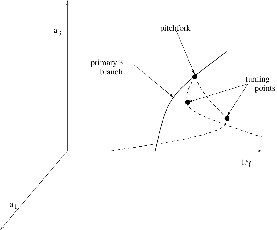
During the process of numerical continuation of branches of solutions, we discovered an interesting “loop” structure connecting each $k$-th and $3k$-th primary branch (see Fig. 1). We give a simple treatment based on Fourier mode truncations. We will investigate the $(1,3)$ bifurcation in detail. By a scaling theorem of Aston [2], the structure of all $(k,3k)$ bifurcations is the same.

As the required computations are pretty involved, we proceed as follows: (1) we use $\alpha$ and $\gamma$ as our parameters; this has the effect of changing hyperbolae into straight lines; (2) we work on the interval $[0,\pi]$, which allows us to get rid of many multiples of $\pi$; and (3) we use MAPLE [17] throughout, particularly its polynomial manipulation abilities, such as the computation of resultants and of Gröbner bases, and polynomial factorization.

Thus, we are looking at

with double Dirichlet boundary conditions.

Since we are close to the $(1,3)$ bifurcation point, we use the ansatz $u=a_{1}\sin(x)+a_{3}\sin(3x)$. Multiplying equation (4.12) by each of $\sin(kx)$, $k=1,\,3$ in turn, integrating from 0 to $\pi$ and simplifying, we get the algebraic system

Let us examine (4.13) in more detail. We need to work out what the curves $\Gamma_{1}$ and $\Gamma_{3}$ look like, and where they intersect. Putting $a_{3}$ ($a_{1}$) to zero in the first (second) of the equations of (4.13) gives that

These curves are plotted in Fig. 5. Thus in the $(\alpha,\gamma)$ plane above $\Gamma_{1}$ there are no non-trivial solutions of (4.13). We see that the $(1,3)$ bifurcation point is at $(\alpha,\gamma)=(9/10,1/10)$ where the two curves intersect.

Now let us see whether (4.13) will give us a loop, and what this loop really means. To have a loop we must have a solution with $a_{1}=0$ and $a_{3}\neq 0$ of equations (4.13).

In other words, we need to solve simultaneously for $a_{3}$ the equations

and

These solutions for $a_{3}$ are the values of $a_{3}$ on the pure $a_{3}$ branch at which a (pitchfork) bifurcation occurs. There are two equations in one unknown, $a_{3}$, so for solvability they define a relation between $\alpha$ and $\gamma$. The form of this relation can be found by taking the resultant of the above two equations with respect to $a_{3}$ and is given by

This straight line of course intersects the lines $\Gamma_{1}$ and $\Gamma_{3}$ at $(9/10,1/10)$ and as the slope is positive, such bifurcation points only exist for $\alpha<9/10$. For example, it can be checked numerically that if $\alpha=8/10$, the (secondary) bifurcation from the $a_{3}$ branch is at $\gamma=.09542483660$.

We now turn our attention to the nature of the “loop”. For $\alpha<9/10$ there is no pure $a_{1}$ branch. The mixed mode branch bifurcates at $\gamma=1-\alpha$; the pure $a_{3}$ branch bifurcates off $\Gamma_{3}$. It has a secondary bifurcation, a pitchfork, in the $a_{1}$ direction, on the line (4.14). One of these branches then hits the primary mixed branch and they disappear in a saddle node bifurcation. In fact, it is possible to work out where the turning points are. They are given by the following relation connecting $\alpha$ and $\gamma$:

Equation (4.15) is obtained as follows: first divide the first of the equations of (4.13) by $a_{1}$ and then compute the purely lexicographic Gröbner basis of these two equations using the ordering $a_{3}>a_{1}$. This results in a basis with two elements for the ideal generated by the two original equations. One of these basis elements is found to be a polynomial in $a_{1}$ only. We can then take the resultant of this polynomial in $a_{1}$ with its derivative to obtain an enormous polynomial in $\alpha$ and $\gamma$, eliminating $a_{1}$. Some of the roots of this polynomial correspond by construction to turning points, so it is just a matter of factorizing the resultant and picking the right term to obtain $P_{1}(\alpha,\gamma)$. If in $P_{1}(\alpha,\gamma)$ we set $\gamma=1/10-\gamma_{1}$, $\alpha=9/10-\alpha_{1}$, we obtain a homogeneous polynomial of degree 4,

If we now set $\gamma_{1}=h\alpha_{1}$, Descartes’ rule of signs tells us that we will have two real solutions $h_{1}$ and $h_{2}$ of $P_{2}(\alpha_{1},h\alpha_{1})/\alpha_{1}^{4}=0$. Using Maple to compute them, we obtain the approximations for the curves of turning points,

In Fig. 5 we plot in (a) $\Gamma_{1}$, $\Gamma_{2}$, the pitchfork bifurcations given by (4.14) and the curves of turning points as determined by (4.15) local to the bifurcation point. We also illustrate schematically the bifurcations in $a_{1}$,$a_{3}$,$1/\gamma$ space.

Remark: this phenomenon can also be analysed in the framework of bifurcations with hidden symmetries [1, 14, 13].

We showed in section 3 that there are wedges $K_{k}$ in parameter space $(\alpha,1/\gamma)$ where both the $kth$ and $(k+1)st$ branches are stable. Unfortunately though this analysis is only local in nature. Local to the bifurcation point our numerics of section 2.1 agrees with the local analysis we have presented. This lends some confidence to the numerics. If we combine the local analysis with our observations from the numerical continuation in Fig. 3, we make the following conjectures.

Conjecture 1. The wedges $K_{k}$ are non-empty for all $\gamma<\gamma_{k,k+1}$. Along the curves $\Gamma_{k+1,k}$, as $\alpha\rightarrow 0$, $1/\gamma\rightarrow\infty$, while along $\Gamma_{k,k+1}$, $1/\gamma\rightarrow\infty$ as $\alpha\rightarrow\widetilde{\alpha_{k}}\neq 0$.

This automatically means that the curves $\Gamma_{k,k+1}$ and $\Gamma_{l+1,l}$ intersect if $l>k$. The upshot of this conjecture is that the different wedges $K_{k}$, $K_{l}$ intersect, and increasingly so as $\gamma\rightarrow 0$, which for each $N$ creates regions of parameter values in which there are $N$ different stable equilibria. This is partially consistent with the Friesecke and McLeod result, at least for $\alpha<\widetilde{\alpha_{1}}$. Furthermore we can give a reformulation of Müller’s conjecture that we stated in the introduction, namely

Müller’s conjecture. All stable equilibria are created by the above mechanism.

The two statements of this conjecture are equivalent as all the stabilized branches have $D_{2k}$ symmetry for some $k$.

To conclude we propose another conjecture.

Conjecture 2. If $\alpha>k^{2}\pi^{2}$, there are no equilibria with less than $(k-1)$ internal zeroes.

This is again based on the local analysis combined with the steady state bifurcation picture given in section 2.1, the hope is this may be easier to prove than the other two. Note that if this conjecture is true, then for $\alpha>k^{2}\pi^{2}$, an initial condition without internal zeroes will have to evolve at least $k-1$ interfaces.

References

- [1] D. Armbruster and G. Dangelmayr, Coupled stationary bifurcations in no-flux boundary value problems, Math. Proc. Camb. Phil. Soc. 101 (1987), 167–192.
- [2] P. Aston, Scaling laws and bifurcations, in: Singularity Theory and its Applications, Warwick 1989, part II, M. Roberts and I. Stewart, eds., Lecture Notes in Mathematics 1463, Springer-Verlag, Berlin 1991, pp. 1–21.
- [3] J. M. Ball, Dynamics and minimizing sequences, in: Problems Involving Change of Type, K. Kirchgässner, ed., Lecture Notes in Physics 359, Springer-Verlag, Berlin 1990, pp. 3–16.
- [4] J. M. Ball, P. J. Holmes, R. D. James, R. L. Pego, and P. J. Swart, On the dynamics of fine structure, J. Nonlin. Science 1 (1991), 17–70.
- [5]
E. J. Doedel, A. R. Champneys, T. F. Fairgrieve, Y. A.
Kuznetsov, B. Sanstede, and X. Wang, AUTO 97: Continuation and
Bifurcation Software for ODEs,
http://www.maths.surrey.ac.uk/personal/st/B.Sandstede/publications/auto97.pdf - [6] J. Ericksen, Equilibrium of bars, J. Elasticity 5 (1975), 191-202.
- [7] G. Friesecke and J. B. McLeod, Dynamics as a mechanism preventing the formation of finer and finer microstructure, Arch. Rat. Mech. Anal. 133 (1996), 199–247.
- [8] G. Friesecke and J. B. McLeod, Dynamic stability of non-minimizing phase mixtures, Proc. Royal Soc. London A 453 (1997), 2427–2436.
- [9] M. Golubitsky and D. G. Schaeffer, Singularities and Groups in Bifurcation Theory, Springer-Verlag, New York 1985.
- [10] M. Grinfeld and A. Novick-Cohen, Counting stationary solutions of the Cahn–Hilliard equation by transversality arguments, Proc. Royal Soc. Edinburgh A 125 (1995), 351–370.
- [11] M. Grinfeld and A. Novick-Cohen, The viscous Cahn-Hilliard equation: Morse decomposition and structure of the global attractor, Trans. AMS 351 (1999), 2375-2406.
- [12] M. Grinfeld and A. Novick-Cohen, in preparation.
- [13] T. J. Healey and U. Miller, Two-phase equilibria in the anti-plane shear of an elastic solid with interfacial effect via global bifurcation, Proc. Royal Soc. A 463 (2007), 1117–1134.
- [14] G. W. Hunt, Hidden (a)symmetries of elastic and plastic bifurcation, Appl. Mech. Rev. 36 (1986), 1165–1186.
- [15] Y. Huo and I. Müller, Interfacial and inhomogeneity penalties in phase transitions, Continuum Mech. Thermodyn. 15 (2001), 395–407.
- [16] W. D. Kalies and P. J. Holmes, On a dynamical model for phase transformation in nonlinear elasticity, Fields Inst. Commun. 5 (1996), 255-269.
- [17] E. Kamerich, A Guide to Maple, Springer–Verlag, New York 1999.
- [18] S. Müller, Singular perturbations as a selection criterion for periodic minimizing sequences, Calc. Var. 1 (1993), 169–204.
- [19] P. J. Swart and P. J. Holmes, Energy minimization and the formation of microstructure in dynamic anti-plane shear, Arch. Rat. Mech. Anal. 121 (1992), 37–85.
- [20] L. Truskinovsky and G. Zanzotto, Ericksen’s bar revisited: energy wiggles, J. Mech. Phys. Solids 44 (1996), 1371–1408.
- [21] A. Vainchtein, Dynamics of phase transitions and hysteresis in a viscoelastic Ericksen’s bar on an elastic foundation, J. Elasticity 57 (1999), 243–280.
- [22] A. Vainchtein, Stick-slip interface motion as a singular limit of the viscosity-capillarity model, Math. Mech. Solids 6 (2001), 323–341.
- [23] A. Vainchtein, T. J. Healey, and P. Rosakis, Bifurcation and metastability in a new one-dimensional model for martensitic phase transition, Comput. Methods Appl. Mech. Engrg. 170 (1999), 407–421.
- [24] A. Vainchtein, T. Healey, P. Rosakis, and L. Truskinovsky, The role of the spinodal region in one-dimensional martensitic phase transitions, Physica 115D (1998), 29–48.
- [25] A. Vainchtein and P. Rosakis, Hysteresis and stick-slip motion of phase boundaries in dynamic models of phase transitions, J. Nonlinear Sci. 9 (1999), 697–719.
- [26] N. K. Yip, Structure of stable solutions of a one-dimensional variational problem, Control, Optim. Calc. Variations 12 (2006), 721–751.