Shear viscosity of a hadronic gas mixture
Abstract
We discuss in detail the shear viscosity coefficient and the viscosity to entropy density ratio of a hadronic gas comprised of pions and nucleons. In particular, we study the effects of baryon chemical potential on and . We solve the relativistic quantum Boltzmann equations with binary collisions (, and ) for a state slightly deviated from thermal equilibrium at temperature and baryon chemical potential . The use of phenomenological amplitudes in the collision terms, which are constructed to reproduce experimental data, greatly helps to extend the validity region in the - plane. The total viscosity coefficient increases as a function of and , indirectly reflecting energy dependences of binary cross sections. The increase in direction is due to enhancement of the nucleon contribution while the pion contribution diminishes with increasing . On the other hand, due to rapid growth of entropy density, the ratio becomes a decreasing function of and in a wide region of the - plane. In the kinematical region we investigated MeV, GeV, the smallest value of is about 0.3. Thus, it never violates the conjectured lower bound . The smallness of in the hadronic phase and its continuity at (at least for crossover at small ) implies that the ratio will be small enough in the deconfined phase . There is a nontrivial structure at low temperature and at around normal nuclear density. We examine its possible interpretation as the liquid-gas phase transition.
I Introduction
Shear viscosity of a hot QCD matter has been attracting much attention in recent years. The major reason for that is the intriguing experimental discovery that the matter created in heavy-ion collisions at Relativistic Heavy Ion Collider (RHIC) in Brookhaven National Laboratory could be close to a perfect fluid RHIC. This unexpected result has driven people to think about strongly-interacting quark-gluon plasma (abbreviated as “sQGP”) which may be realized at temperature just above the critical temperature . As a result of strong-coupling nature, sQGP is thought to have very small shear viscosity, which is however not directly confirmed yet in a satisfactory way. In fact, only a few things are understood about sQGP because we will not be able to investigate it within standard perturbative QCD techniques. The only technique available now (except for lattice simulations which are not analytic methods) is the one based on the AdS/CFT correspondence, which relates strongly-coupled supersymmetric Yang-Mills theories to weakly-coupled gravity theories.
There is an interesting outcome from the AdS/CFT analysis in relation to the shear viscosity: It has been conjectured that there would be a lower bound in the “shear viscosity coefficient to the entropy density ratio” (or simply the “viscosity to entropy ratio”) KSS. We call this “the KSS bound” after authors’ names of Ref. KSS. The lowest value is satisfied by several super Yang-Mills theories in the large limit (strong coupling limit), which suggests that the bound could be universal. Of course, there is no guarantee for this bound to hold in real (non-supersymmetric) QCD whose gravity dual is not found, but interestingly enough, the values of extracted from RHIC experiments Gavin and from lattice simulations Nakamura; Meyer seem to be small enough and close to the lower bound.
On the other hand, there is an important empirical observation which can be seen in many substances such as helium, nitrogen, and water: The ratio has a minimum at or near the critical temperature Kapusta (see also Hirano). More precisely, the ratio shows a cusp at for the first order transition, while it has a convex shape for the crossover with its bottom around the (pseudo) critical temperature. Since this behavior is observed in many substances, it is expected to be universal. Recall that the phase transition in QCD is most probably crossover at least for low densities. Therefore, what we naturally expect for the QCD matter from the two observations mentioned above is that the ratio will have the minimum at , and the numerical value at that point will be close to the KSS bound . It is of primary importance to check whether this expectation is indeed the case or not, and to understand the properties of the QCD matter around not only for . These considerations motivated us to investigate the shear viscosity in QCD from the hadronic phase . Notice that we can indirectly study the properties of sQGP from below because physical quantities such as the ratio will be continuous at for the crossover transition.
Transport properties of a meson gas have been studied by several people. Many of the calculations are based on the Boltzmann equations with the Chapman-Enskog method which is a standard approach for weak dissipative phenomena, especially for computing transport coefficients deGroot. Differences among several papers Gavin2; Prakash; Davesne; Dobado1; Dobado2 include kinetic or statistical properties of particles (relativistic or nonrelativistic, quantum or classical), species of mesons (pions, kaons, etc.), and the cross sections in the collision terms. For example, Ref. Dobado1 treated a nonrelativistic quantum pion gas with the binary cross section given by the leading order chiral perturbation theory (LO-ChPT). Recently, similar problems have been revisited in relation to the KSS bound Chen1; Dobado3. In Ref. Chen1, the ratio computed with the cross section in LO-ChPT turned out to violate the KSS bound for temperature beyond MeV, and it was speculated that such violation could be related to the existence of phase transition. However, soon after that, it was shown in Ref. Dobado3 that the KSS bound is not violated in a pionic gas if one computes the shear viscosity with a phenomenological cross section using the experimental phase shifts. What we have learned from these papers is the following: (i) we have to be careful when we use the cross section from effective field theories, and (ii) the ratio of a relativistic pion gas is small enough at relatively large temperature , but does not violate the KSS bound .
At this point, there comes a natural question: how does change if one adds nucleons to the pure pion gas? Naively, we expect that the ratio will decrease as number of nucleons is increased because the pion cross section will effectively enhance in the presence of nucleons, yielding smaller shear viscosity, while the entropy will increase. Thus, there is a chance that the ratio could violate the KSS bound if the bound does not change. Notice that the pion-nucleon gas is the minimum requisite which allows us to study the effects of baryon chemical potential . Therefore, it is quite interesting and important to investigate the dependence of in the pion-nucleon gas. Such investigation will also urge people to study the (possible) -dependence of the KSS bound. In fact, the “universality” of the KSS bound has not been tested at finite baryon chemical potential.
Most recently, the authors of Ref. Chen1 have applied their framework to the pion-nucleon gas to study the behavior of in the - plane Chen2. However, their focus was not on the KSS bound but on the new finding: a valley structure in at low temperature and large chemical potential which they argued would correspond to the nuclear liquid-gas phase transition. Although this is a very interesting suggestion, their results should be critically checked since they are based on the effective field theories whose validity region is severely limited. On the other hand, a realistic calculation of the viscosity in the pion-nucleon gas was performed some time ago by Prakash et al. Prakash. Remarkably, they used the binary cross sections in the collision terms, which roughly reproduce experimental data. However, unfortunately, the dependence on baryon chemical potential was not investigated in detail. Besides, this calculation is based on classical Boltzmann equations, and thus cannot be applied to relatively large chemical potential where the effects of Fermi statistics is expected to be large.
In view of the present situation mentioned above, what we should do is rather evident: for the purpose of studying the dependence of the shear viscosity and the ratio in a pion-nucleon gas, we treat the relativistic quantum Boltzmann equations with binary cross sections which are determined to reproduce experimental data. We are very careful about the range of validity of our framework. We also check whether the valley structure found in Ref. Chen2 indeed exists even with the phenomenological cross sections. It is also important to compare our results with those from hadron cascade simulations. For example, the shear viscosity coefficient is computed for a meson gas in Ref. Muronga and for a meson-baryon gas in Ref. Muroya.
The paper is organized as follows: in the next section, we explain the relativistic quantum Boltzmann equations for a dilute pion-nucleon gas, and define the cross sections we use in the collision terms. We treat the small deviation from the thermal equilibrium to the linear order (the Chapman-Enskog method), and give the shear viscosity coefficient through the solutions to the Boltzmann equations. In Sect. III, we present our numerical results for a pure pion gas and a pion-nucleon gas mixture. We introduce a criterion which measures the validity region of the calculations. The use of phenomenological cross sections is very important to enlarge the range of validity. We discuss in detail the effects of chemical potential on and and examine the interpretation of the valley structure as the liquid-gas phase transition. Summary is given in the last section.
II Kinetic theory of a hadronic gas mixture
II.1 Quantum Boltzmann equations
We first explain our theoretical framework which is necessary for computing the shear viscosity coefficient. Consider a dilute gas of pions () and nucleons () in which particles interact with each other through binary collisions. Nonequilibrium processes such as relaxation to thermal equilibrium can be described by kinetic equations for one particle distribution functions and (below, we suppress -dependence). For simplicity, we assume that the gas is isospin symmetric, and thus and are isospin averaged distributions. The relativistic quantum Boltzmann equations (more precisely, the Uehling-Uhlenbeck equations) of this hadronic gas mixture are then given by
| (1) | |||
| (2) |
where and the collision terms are defined as
| (3) | |||||
| (4) | |||||
We have used shorthand notation and are the degeneracy factors , . For the collisions between the same species (, ), we have added a factor . The factors and represent the Bose-Einstein and Fermi statistics of particles, respectively. Finally, in the integrants are invariant measures with the scattering amplitudes squared: For example,
| (5) |
where is the elastic scattering amplitude for . Explicit form of the scattering amplitudes will be shown at the end of this section. These are the basic ingredients of the kinetic theory.
Before we discuss how to solve the Boltzmann equations (1) and (2), we need to know the equilibrium states. We define them without solving the full Boltzmann equations: They are given by the distributions which make the collision terms vanish. Namely, . These conditions are easily satisfied by the following Bose-Einstein and Fermi-Dirac distributions if the common temperature and hydrodynamic velocity are used
| (6) | |||||
| (7) |
where is the baryon chemical potential. The parameters , and can, in principle, depend on the coordinates (local equilibrium), but when we compute quantities in thermal equilibrium, we simply select the rest frame so that .
In evaluating the entropy density, we use the expression in the equilibrium state as is done in the literature because the deviation from the equilibrium is assumed to be small. Namely, by using the grand partition functions for and ,
| (8) | |||
| (9) |
one obtains the total entropy density as follows:
II.2 Shear viscosity coefficient
The shear viscosity coefficient is defined through the deviation of spatial components of the energy momentum tensor in the linear order with respect to fluctuation from the equilibrium. Consider a nonequilibrium state which is slightly deviated from the global equilibrium. Small deviation of the space components of energy momentum tensor can be divided into traceful and traceless parts:
| (10) | |||||
| (11) |
where is a space component of the hydrodynamic four velocity (which is common for and )
Eq. (10) is the definition of the shear and bulk viscosity coefficients and . The flow vector , as well as and , is in principle arbitrary and can depend on spatial coordinates. But below we consider the case where only the flow vector depends on the coordinates, and in particular, its divergence is vanishing: and . This situation corresponds to considering only the shear viscosity coefficient and ignoring all the other transport coefficients such as bulk viscosity or heat conductivity.
If one knows distributions as the solutions to the Boltzmann equations (1) and (2), one can explicitly compute the (deviation of) energy momentum tensor:
| (12) | |||||
As mentioned above, we consider only the deviation that originates from the shear. Then, it is quite convenient to parametrize and as follows ():
| (13) | |||
| (14) |
where we have introduced new quantities to be determined by the Boltzmann equations.
Substituting Eqs. (13) and (14) into Eq. (12) and comparing the result with Eq. (10), one finds the shear viscosity coefficient as a function of unknown functions :
| (15) | |||||
The unknown functions (or equivalently, the deviations ) are numerically determined by solving the Boltzmann equations that are linearized with respect to . This procedure corresponds to the lowest order Chapman-Enskog method. Here we discuss only the outline of the procedure to solve the Boltzmann equations. More details are discussed in Appendix B.
After the linearization, the Boltzmann equations (1), (2) become a coupled linear equations for and . Following Ref. Dobado1, we solve these equations in the functional space spanned by the orthogonal polynomials . Let us expand by these bases:
| (16) |
where is a polynomial of the order , and is the coefficient independent of . Notice that and are not equivalent to each other. Indeed, they are defined so that they satisfy the following different orthogonal conditions:
| (17) |
| (18) |
The normalization factors and are not chosen to be 1. Instead, we choose the polynomial so that the coefficient of the term with the highest degree is unity (such polynomials are called ”monic”). Namely, the first three polynomials have the following form:
Parameters , and are uniquely determined by the orthogonal conditions (thus independent of the dynamics). In fact, has unknown parameters, which are uniquely determined by orthogonal conditions with lower polynomials (). Thus, and in Eqs. (17) and (18) are known after we completely determine . Practically, the expansion (16) is well approximated by the first few terms. Thus, in the present analysis, we take only the first three terms:
| (19) | |||
| (20) |
where we have used the definition . The coefficients are numerically determined. Once we know these coefficients, we can compute the shear viscosity coefficient from Eq. (15). We have checked that the results do not change even if we take up to the fourth terms .
Two comments are in order about our formulation. Firstly, we recall that the expansion of in Eq. (16) is a familiar technique in solving the Boltzmann equation by the Chapman-Enskog method. If one treated a classical Boltzmann equation, measure of the orthogonal condition would be given by a much simpler distribution, the Maxwell-Boltzmann distribution. In this case, the polynomials that satisfy the orthogonal condition are given by famous functions, the Sonine polynomials Chapman. For the quantum Boltzmann equation, however, the measure in the orthogonal condition is given by either the Fermi-Dirac or Bose-Einstein distribution, as shown in Eqs. (17) and (18). In this case, the polynomials satisfying them are not known, and we have to find them order by order.
Secondly, note that the shear viscosity coefficient defined by Eq. (15) may be formally written as
| (21) |
It apparently looks ‘additive’ with respect to each contribution. Indeed, if one considers a pion gas system without nucleons, one finds exactly the same expression as the first term of Eq. (15). One might then be tempted to conclude from the expression (21) that the inclusion of nucleons always contributes to enhance the value of shear viscosity. However, such argument does not make sense because the function itself will change by the inclusion of nucleons. We will see later that indeed decreases as the effects of nucleons become large (i.e., with increasing chemical potential).
II.3 Scattering amplitudes of binary collisions
Let us show the explicit expression of the scattering amplitudes in the collision terms (3), (4), and (5). Note that we have assumed factorization of the scattering amplitudes from the products of one-particle distributions in the collision terms. This is physically natural in a dilute gas where each collision is simply treated as an independent binary collision (ignoring higher order multiparticle correlations). Therefore, as long as we consider a dilute gas system where the Boltzmann equation is applicable, it is reasonable to use the amplitudes for two particle scatterings in the vacuum (free space). This is a great merit in computing transport coefficients. If one follows the microscopic Kubo formula to compute the transport coefficients, it is quite nontrivial how to include the effects of physical processes. On the other hand, if one uses the Boltzmann equation, one can easily incorporate the physical cross sections in the collision terms, which is however less justified from the first principle. In the present paper, we examine two different parametrizations for the scattering amplitudes. One is based on theoretical calculations, while the other is constructed from the experimental data. More precisely, we use the amplitudes from the low energy effective field theory (EFT) on the one hand, and the phenomenological amplitudes designed to reproduce experimental data of the elastic scatterings on the other hand.
Scattering amplitudes based on EFT are the following. First of all, the isospin-averaged scattering amplitude is given by the leading order Chiral Perturbation Theory (LO-ChPT) Weinberg:1978kz:
| (22) |
where is the pion decay constant ( MeV), and are the Mandelstam variables for the scattering .
Next, for the scattering, we use the results of low energy effective theory (LO heavy baryon ChPT) Fettes:1998ud. The isospin averaged scattering amplitude in the Center-of-Mass (CM) frame is
| (23) |
where and are, respectively, the magnitude of pion momentum, and the scattering angle in the CM frame. Two functions and are
where is the nucleon axial charge, and is the pion energy in the CM frame. Note that the overall factor in Eq. (23) is not the same as in Ref. Chen2 though both are based on Ref. Fettes:1998ud. This is because we have used the standard normalization factor for the spinors instead of which was adopted in Ref. Fettes:1998ud.
Lastly, let us consider the scattering. In the low energy EFT, scattering amplitudes in the CM frame for fixed spin and isospin can be parametrized in terms of the scattering length and the effective range as
| (24) |
where is the magnitude of nucleon momentum in the CM frame. For each process, parameters and are determined to fit the low energy experimental data with the contribution from Coulomb force removed. Their numerical values are shown in table I. They are taken from Ref. scef:
| system | parameter | ||
|---|---|---|---|
| (fm) | —– | ||
| 2.79 (fm) | —– | ||
| (fm) | —– | ||
| 2.84 (fm) | —– | ||
| (fm) | 5.42 (fm) | ||
| 2.73 (fm) | 1.73 (fm) |
In low energy scattering, the dominant contribution to the amplitude is given by the -wave (orbital angular momentum ). Thus, we construct the spin-isospin averaged scattering amplitude from the expression (24) for the -wave with appropriate weight factors of spin and isospin. Details of the spin-isospin average are explained in Appendix A.


In summary, the scattering amplitudes based on EFT are given by Eqs. (22), (23), and (24). It should be emphasized that all these expressions of the scattering amplitudes are valid only in a limited region of kinematics. LO-ChPT (for case) is usually considered to be valid for 1 GeV with being the magnitude of pion momentum. In the heavy baryon ChPT for the case, there is an additional expansion parameter , which gives almost the same limitation as for the case. Lastly, for the case, the differential cross section (24) is valid only for small , or equivalently, small scattering energy near the threshold. This fact implies that the validity of results derived from the Boltzmann equations will also be restricted to a small region in the - plane, as we will discuss later.
With this limitation in mind, it is quite important to consider physical scattering amplitudes in order to check the usefulness of, or more importantly to go beyond, the low energy EFT. To this end, we have constructed phenomenological amplitudes from the experimental data (differential cross sections) by fitting the coefficients of the partial-wave expansion. The fit was performed to the data up to GeV ( MeV) in the scattering, GeV ( MeV) in the scattering, and GeV ( MeV) in the scattering. Details of the fitting procedure are discussed in Appendix A. In Fig. 1, we compare elastic cross sections of the two different parametrizations. The elastic cross sections from the phenomenological amplitudes are almost identical with the experimental data (not shown) in the energy regions shown in the figures. Peaks in and cross sections are -meson and resonances, respectively. As mentioned above, the range of validity of LO-ChPT (for cases) is 1 GeV for the pion momentum. Thus, if one applies this limitation to the momentum of colliding particles in the CM frame, one finds for the scattering energy with GeV for the scattering, and 2.4 GeV for the scattering. Indeed, as evident from the figure, deviation of LO-ChPT from the phenomenological cross sections is already sizable well below the upper limits (mainly because of the -meson and resonances). For example, in the case, LO-ChPT gives the same tendency as the phenomenological cross section up to MeV ( MeV), but beyond that the deviation is not small. Therefore, it would be safe to consider the validity region of LO-ChPT to be
| (25) |
which is of course within GeV. Later we will use this limit to evaluate the maximum temperature up to which LO-ChPT is applicable. From the figures, it is obvious that the difference of two parametrizations becomes larger and larger with increasing energies. The and cross sections from LO-ChPT monotonically increase and become too large compared to the actual physical cross sections. We will see in the next section that this difference greatly affects the numerical value of the shear viscosity.
III Numerical results
III.1 Pion gas
Let us first discuss the case with only pions. This is important for properly understanding the effects of nucleons in the next subsection and, at the same time, for checking the validity of our calculation compared with the existing results Chen1; Dobado3. As we mentioned before, our formalism for the gas can be easily reduced to the case with only pions (by setting the nucleon degeneracy factor , for example). Then, the shear viscosity coefficient is given by the first term of Eq. (15), and we determine by solving the Boltzmann equation (1) with the collision term given by the first term of Eq. (3). The expansion of with respect to the orthogonal polynomials was taken up to the third order to ensure the convergence of the result.
III.1.1 Range of validity
Before presenting our numerical results, we clarify the range of validity in temperature for two parametrizations of the scattering amplitudes. As we already specified in Eq. (25), LO-ChPT is valid only in a limited kinematical regime: MeV, while the phenomenological amplitude is by construction valid up to GeV. These conditions can be translated to the limitation in temperature in the following way. Consider the binary collisions in thermal equilibrium. Since each collision takes place between particles in thermal equilibrium, the scattering energy squared will fluctuate around its mean value with a width . The average and the width (standard deviation) may be defined by
| (26) | |||
| (27) |
Because the scattering energy squared of most of the collisions are below , one can regard as (a measure of) the highest energy squared at temperature . So, one may interpret the validity condition of LO-ChPT as GeV2, and thus obtain the validity condition for temperature with given by GeV2. In Fig. 2, we show and as functions of temperature. From the figure, one can read MeV. Therefore, we may conclude that the results of LO-ChPT are reliable only up to MeV. On the other hand, the phenomenological amplitude is valid up to GeV2. Therefore, we expect from the figure that the results of the phenomenological amplitude will be reliable up to temperature close to MeV.


There is another important check for the validity of our framework. It is the applicability of the Boltzmann equations. Recall that in deriving the Boltzmann equations, one assumes that a two-point correlation function can be factorized into a product of two one-point functions (one particle distributions ). This is physically acceptable when the density of particles is small enough. This condition is normally expressed as
| (28) |
where is the mean-free path
| (29) |
with being the cross section, and is the interaction range, meaning that each collision takes place independently. If we define the interaction range by the Compton length of pions: , then the validity condition for the Boltzmann equation reads . Alternatively, if we define through the cross section as , we obtain another expression . Both expressions give similar restriction on temperature. Figure 3 shows the ratio as a function of temperature, where the (phenomenological) cross section is estimated by its thermal average. One finds at MeV, which manages to satisfy the inequalities. At this temperature, the mean-free path of pions is estimated as fm, which is consistent with the literature MFPath. As the temperature is decreased, the mean-free path becomes longer, and the Boltzmann description gets better and better.
Combining these two results, we may conclude that the phenomenological analysis of a pion gas based on the Boltzmann equation will be valid up to temperature MeV which is much higher than the LO-ChPT limit MeV, but lower than the critical temperature MeV. However, we notice that there is a caveat to this conclusion. In fact, even though we have satisfactory description of scatterings in wider kinematical regime, we have to worry about at least two other effects as temperature increases. The first one is the effects of other (heavier) degrees of freedom such as kaons, and the second is the possible modification of pions in thermal enviornment. Both are however beyond the scope of the paper and we leave them for future problems.
III.1.2 Shear viscosity coefficient
Figure 4 shows the shear viscosity coefficient as a function of temperature . Open diamonds () and open triangles () are based on numerical solutions to the Boltzmann equations with the phenomenological amplitudes and LO-ChPT, respectively. Remarkably, the two results show quite different behavior. While the result of LO-ChPT decreases with increasing , that of the phenomenological amplitude shows the opposite behavior.
Qualitative behavior of two different results can be easily understood by using rough estimate of the viscosity coefficient. In classical transport theory for a dilute gas of one component, the shear viscosity coefficient is expressed in terms of the mean-free path , Eq. (29), as follows:
| (30) |
where is the particle number density, is the average momentum, and is the binary cross section. Thus, the shear viscosity coefficient is inversely proportional to the cross section. As we already saw in Fig. 2, the typical energy in the scattering increases with temperature. This means that average cross section indirectly depends on temperature. Notice also that the average momentum roughly increases like (because ). Therefore, temperature dependence of the shear viscosity coefficient is essentially determined by the interplay between those of and . For example, if the average cross section increases rapidly as a function of (faster than ), is a decreasing function of . But if is almost constant, is an increasing function of . Based on these considerations and Fig. 1, we can easily deduce the followings: As for the temperature dependence of the shear viscosity, we expect that is slightly smaller than at low temperature (because ), while at high temperature. More precisely, since of the ChPT monotonically increases as while that of the phenomenological amplitude does not grow, we expect that the shear viscosity decreases in the ChPT case while the opposite happens in the phenomenological case.

Now let us come back to Fig. 4, where we also show the rough estimate (30) with two different parametrizations. For the (average) cross section in the rough estimate (30), we evaluate it at the average momentum , i.e., .11 1 One can evaluate by its thermal average similarly as in Eq. (26), but the qualitative behavior is the same as . Comparing the results of the Boltzmann equations and of the rough estimate (30), we find that qualitative agreement of the results in two different ways of computation. Nontrivial behavior of the rough estimate for the phenomenological amplitude (filled diamond points) is due to the resonance shape of the elastic cross section in Fig. 1. Indeed, the valley around MeV corresponds to the meson peak around GeV2 in the cross section (According to Fig. 2, GeV2 is translated into MeV, which is further diminished due to in the numerator of ). In the Boltzmann equations, such structure is further washed out by thermal average. From these analyses, we now understand that the behavior of the numerical results of the Boltzmann equations is largely due to the energy dependence of the cross sections used in the collision terms. In particular, the decreasing of LO-ChPT at relatively high temperature MeV is an artifact of too large cross section outside of the validity region of LO-ChPT. On the other hand, our most reliable result (open diamonds in Fig. 4) shows linear increase with temperature for MeV. This behavior is consistent with that of hadronic resonance gas models Gyulassy; Gavin2. Moreover, our result is also consistent with that of Ultrarelativistic Quantum Molecular Dynamics (UrQMD) for a meson gas Muronga, which also gives linear dependence on , and GeVfm GeV-3 at MeV.
III.1.3 The ratio

Figure 5 shows our numerical results of the ratio as a function of temperature . Dashed and solid lines correspond to the results of LO-ChPT and the phenomenological amplitude, respectively. In both cases, is a monotonically decreasing function of . Notice that the result of LO-ChPT violates the conjectured bound (the KSS bound, shown as the dotted line) at around the critical temperature MeV. On the other hand, from the phenomenological amplitude keeps well above the KSS bound up to temperature . These are consistent with the results of Refs. Chen1; Dobado3.
Since the entropy density is common in both cases , behavior of can be understood by that of itself. For example, we saw that decreases in LO-ChPT, while it increases in the phenomenological case. Such difference affects on the ratio : it decreases faster in the LO-ChPT case than in the phenomenological one. Also there is a crossing point for the two results of at MeV (see Fig. 5), and this point coincides with that of the shear viscosity (see the open diamonds and open triangles in Fig. 4).
It has been argued in Ref. Chen1 that violation of the KSS bound suggests the existence of phase transition (or crossover transition) in order for the KSS bound to remain valid. This kind of argument is of course dangerous because the precise value of depends on the amplitude in the collision term, and the result of Ref. Chen1 is based on LO-ChPT, whose applicability is limited to MeV as we already discussed in detail. In fact, more reliable result with the phenomenological amplitude does not violate the KSS bound even around the critical temperature. Therefore, “violation of the KSS bound” cannot be the signature of phase transition. Instead of seeing violation of the KSS bound, we propose to check the other property to catch the indication of phase transition. As we mentioned in Introduction, Ref. Kapusta suggests that the ratio has a minimum around the (pseudo-) critical temperature . If this is indeed the case, it implies that (for crossover transition) the curve of as a function of temperature will have a convex form around , and the slope will decrease as temperature approaches from the left. (This kind of argument will hold as far as the temperature is not too far away from the critical end point.) What we observed in Fig. 5 for the phenomenological amplitude is indeed the decrease of the slope with increasing temperature. Thus, even if the ratio is still well above the conjectured bound, we can anticipate the existence of phase transition.

In Fig. 6, we show the (absolute value of) slope of the ratio for the phenomenological amplitude. Recall that we have estimated the border of validity region of our calculation to be MeV. Thus, we use the results around MeV for linear extrapolation towards higher temperature. More precisely, we approximate the curve around at some temperature as
| (31) |
Then the slope is approximated by a linear function of . The critical temperature may be defined by the temperature where the slope is zero: . Namely,
| (32) |
where and on the left-hand side of a convex function . The result of linear extrapolation at MeV is shown on the same figure. Remarkably, the temperature at which the straight line cuts the horizontal axis is 173 MeV, which is quite a reasonable result as the critical temperature. In addition to this, one can guess the value of at by using the approximation (31):
| (33) |
If one substitutes numerical values at MeV, namely, , MeV-1 and MeV-2 which are read from Figs. 5 and 6, one finds at . These results should be understood with reservation at least for two reasons. First of all, there is ambiguity in the choice of , which will affect the values of and . However, in fact, cannot be taken arbitrary because we need to take as close to as possible for the linear extrapolation to be accurate. To obtain reasonable values of and , the largest possible value for is preferable. Since the choice 140 MeV is the upper limit of our validity region, we expect that the estimated value MeV is the best value of our calculation. Therefore, even if there might be some ambiguity in selecting , we can say that we have chosen the best value. The second source which might change the values of and is the possible contributions from heavier mesons. Since such contributions become more important as , our results with only pions become better as we depart from (which is however not desirable for determination of ). Still, we expect our results are not so bad because at MeV such heavier particles can be ignored, and even at MeV, number of kaons amounts to only 20% of total particles.
For the crossover transition, the ratio will be continuous at the (pseudo) critical temperature . This immediately implies that the numerical value of determined above is relevant even in the deconfined phase. Our result is well above the KSS bound, but is small enough compared to the weak-coupling QCD result (see for example, Fig. 4 of Ref. Kapusta). In this sense, the QCD matter around could be “strongly interacting”. However, we should be careful when we draw such a conclusion from the value of . In fact, the smallness of the ratio is not a direct consequence of large cross section which may be realized by a strongly interacting matter. In our calculation with the phenomenological amplitude, the cross section does not grow a lot (in contrast with the LO-ChPT) and the viscosity even increases as . Still, since the entropy increases faster than , the ratio becomes a decreasing function of temperature. Therefore, the smallness of the ratio is realized in a nontrivial way.
III.2 Pion-nucleon gas
Let us now present the numerical results for a dilute gas. As advocated in Introduction, addition of nucleons to a pion gas enables us to study the effects of baryon chemical potential. We discuss how the results of a pion gas presented in the previous subsection change under the influence of the chemical potential.
III.2.1 Range of validity
We start again by the discussion on the range of validity of our framework. Since we have to take the and collisions into account in the gas, we introduce the average scattering energy squared between particles and ( or ):
| (34) |
For the scattering, this is of course equivalent to Eq. (26) and depends only on . But for the and scatterings, the average values depend on both and . Similarly as before, we further define the standard deviation by , and regard as a measure of the highest energy of the scattering at temperature and baryon chemical potential .

In Fig. 7, we show the values of on the - plane. Recall that the fit to experimental data in the scatterings is by construction valid up to GeV2. However, in fact, our parametrization works well up to slightly higher value GeV2. Therefore, we define the borderline of the validity region by temperature and chemical potential that satisfy GeV2. The result is shown on the same figure 7 by a thick solid curve. The maximum temperature is about 130 MeV or slightly smaller than that, while the chemical potential is not restricted up to GeV. If we perform the same analysis for the scattering, the borderline defined by GeV2 locates outside of the region of our interest MeV, GeV. On the other hand, the validity region of the low energy EFT is severely restricted. For example, if we take the maximum value of to be 1.88 GeV (beyond which the phenomenological fit starts to deviate from the low energy EFT fit, see Appendix A), then the borderline defined by GeV2 is very close to the horizontal axis (see Fig. 7). Even if we relax the condition to higher value GeV2, allowed region is still very narrow.

Let us also examine the validity condition for the Boltzmann equations. The criterion is again given by Eq. (28), but now pion’s mean-free path should be modified in the presence of nucleons, and we have to separately consider nucleon’s mean-free path, too. According to classical transport theories, the mean-free path of -th component in a mixed gas is modified as Kennard
| (35) |
where is the mean-free path of a pure gas of -th component, and is the cross section between -th and -th components. Therefore, the mean-free paths of pions and nucleons are respectively given by
| (36) | |||
| (37) |
Consider the condition for nucleons. If one takes mb as a typical value of the cross section (twice of the saturating value at high energy, see Fig. 1) and uses again for the interaction range, then the condition for nucleons can be estimated as with fm-3 being the normal nuclear density. This condition is physically quite reasonable since we do not expect standard Boltzmann description useful at normal nuclear matter density. To obtain more precise restriction depending on and , we need to use Eqs. (36) and (37) and estimate each condition by replacing and by their thermal averages. In Fig. 8, we show the lines for several values of the ratio in the - plane. For simplicity, we used for both pions and nucleons. In the region of low baryon density where pions are dominant degrees of freedom for transport phenomena, we show the ratio for pions . The line for (solid line) is consistent with the previous result shown in Fig. 3. We may regard this line as the border of the validity of the Boltzmann equations at low densities. On the other hand, at large chemical potential and low temperature, transport phenomena is dominated by nucleons. The lines for the ratio are shown in the figure. We may again regard the line as the borderline, which reaches at . This condition is more restrictive than that of Fig. 7.
Combining these two analyses, we may conclude that our framework is valid in a wide region of the - plane, whose boundary is roughly given by (a quarter of) the elliptic curve connecting (130MeV, 0) and (0, 950MeV). The first point (130MeV, 0) is specified by the measure of the highest scattering energy squared, and the last point (0, 950MeV) is from the validity limit of the Boltzmann equations.
T = 50 MeV T = 100 MeV


III.2.2 Shear viscosity coefficient
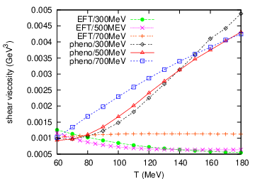
In Fig. 9, we show temperature dependence of at different values of chemical potential MeV. Comparison is made between the results of the low energy EFT and the phenomenological amplitudes. These temperature dependence is qualitatively consistent with the previous results of the pion gas (see Fig. 4). As for the dependence, however, the shear viscosity coefficient shows nontrivial behavior. In particular, in the window 80 MeV 130 MeV, it increases with increasing . This is not quite understandable at first because we expect that the cross section of scattering will effectively enhance in the presence of nucleons while the effects of nucleon viscosity may be ignored at lower density, meaning that the shear viscosity will decrease. To understand what really happens when , let us again consider a rough estimate of the shear viscosity of a mixed gas. Let the shear viscosity coefficient of a pure gas of particle species be where is the number density, is the average momentum, and is the mean-free path. Then the shear viscosity coefficient for component gas is given by the sum of each viscosity with modified mean-free path given in Eq. (35) Kennard:
Thus for the gas mixture, we obtain
| (38) | |||||
where we have used the approximation . In the two extreme limits and , the formula (38) reduces to and , respectively. Therefore, this formula interpolates a pure pion gas at low and a pure nucleon gas at high . Notice that the pion contribution is always smaller than due to the presence of interaction, as we alluded before in relation to Eq. (21). This is exactly what we expected. On the other hand, it is not straightforward to predict the behavior of the total shear viscosity. If one plots the rough estimate (38) as a function of assuming that the cross sections are constant and are of the same order, one finds that decreases at small values of (small ), but turns into increase at large (large ). If one changes the numerical value of cross sections a little, then the curve turns into monotonic increase. In fact, both can happen in reality depending on temperature. In Fig. 10, we have plotted at MeV and 100 MeV as a function of . While the total viscosity behaves differently in these two panels, one can see monotonic decrease (increase) of (), namely, the interplay between and at both temperatures. Therefore, the increase of with increasing observed in Fig. 9 can be understood as a result of enhancement of .
III.2.3 The ratio


Figure 11 shows temperature dependence of the ratio of the gas at different values of baryon chemical potential MeV. The left-hand side is the results of the low energy EFT, while the right-hand side, the phenomenological amplitudes. The ratio shows qualitatively the same behavior as in the pion gas system (Fig. 5): (i) Both the results (EFT and phenomenological amplitudes) are monotonically decreasing functions of , (ii) at lower while opposite at higher , and (iii) the ratio of the EFT violates the KSS bound at around while that of the phenomenological amplitudes does not. Notice that the inclusion of chemical potential works to reduce the value of . As a result, for the ratio of the EFT, the temperature at which the curve cuts the KSS bound becomes smaller. On the other hand, for the result of the phenomenological amplitudes, the flattening of the curves seems to occur at lower temperature with increasing . If this is indeed the symptom of crossover transition as we discussed before, one can say that the (pseudo) critical temperature will decrease with increasing , which is consistent with what we know from lattice simulations or effective models. 22 2 One can try to determine the values of from the slope of each curve as in the pion gas case, but we do not perform such extrapolation for two reasons: First, it is practically very difficult to obtain reliable results since the highest temperature allowed for the Boltzmann equations gradually decreases with increasing , as shown in Fig. 8. Second, the chiral phase transition at moderate values of will be most likely of the first order, for which the ratio will show a discontinuity and the slope will not necessarily zero at . Position of the critical end point may be detected from the behavior of the ratio endpoint, but we do not expect our Boltzmann equations can describe the precise structure of the phase transition. We will discuss similar problems in relation to the nuclear liquid-gas phase transition in Sect.III.B.4.
Our result at and MeV is consistent with that of “URASiMA” (Ultra-Relativistic AA collision Simulator based on Multiple scattering Algorithm)Muroya which is a Monte-Carlo event generator of hadronic collisions. It includes both elastic and inelastic scatterings whose cross sections are given by experimental data. The numerical coincidence of the ratio from different frameworks is very interesting. In fact, the essential difference of URASiMA from our framework is the presence of inelastic collisions. But as far as we consider small deviation from thermal equilibrium, inelastic collisions which will change particle numbers (such as or ) would not be so important, and it seems reasonable to obtain the same result from two different frameworks.
Phenomenological


As we already saw in Fig. 9, the shear viscosity coefficient increases in the window 80 MeV130 MeV with increasing . However, in the same window, the ratio does decrease. This clearly implies that the reduction of at MeV is due to the increase of entropy.
In Fig. 12, we show the dependence of the ratio at temperature MeV (left) and at low temperature MeV (right). Recall that the ratio decreases with increasing in Fig. 11 where MeV was shown. This is consistent with the left figure, and in agreement with our original expectation as we mentioned in Introduction. On the other hand, the right figure shows a new structure: There is a valley at large MeV. We will discuss later the physical implication of this structure.
Let us comment again the point made in the last paragraph of the previous subsection. The ratio becomes less than 0.3 at MeV and MeV. This is small enough and is close to the KSS bound compared to other systems such as water. However, as shown in Figs. 9 and 10, the shear viscosity itself grows as the system approaches phase boundary (). Therefore, even if the ratio is small enough, the system cannot be treated, strictly speaking, as a perfect fluid with . Sometimes ideal hydrodynamics is used to describe the matter after hadronization in heavy-ion collisions, but one will have to take into account the effects of viscosity for a realistic simulation.
III.2.4 Valley structure at large and low
In the right panel of Fig. 12
(low temperature MeV), we pointed out
a valley structure at high baryon chemical potential,
which was not seen in higher temperature (left panel).
Let us look at this new structure in more detail and
examine its possible interpretation.
We recall again Ref. Kapusta, where it was suggested that
the ratio would give a minimum at the phase transition
temperature. If this is true for other control parameters,
in particular, chemical potential, and if there is phase transition
under the change of chemical potential, it is natural to
expect that the ratio would exhibit a valley structure
with its minimum at the critical chemical potential .
In other words, if one finds
a valley structure in the direction, one can expect
some kind of phase transition around the minimum. This is what
we observed in Fig. 12. Then, what kind of
phase transition could be related to this valley structure?
The valley locates at low temperature MeV and
at high chemical potential MeV (which is however
not enough for the quark-hadron phase transition).
This is the region where we can see the
liquid-gas phase transition. 33
3
Notice that all
the examples (except for the QCD phase transition)
discussed in Ref. Kapusta are about the liquid-gas
phase transitions. At low MeV and around normal nuclear density,
there is a critical line (possibly first order) separating
a nucleon gas phase and a nuclear matter (liquid). This line
terminates at around MeV Liquid-gas,
and above that temperature,
there is no distinction between a gas and a liquid. Therefore,
if the valley indeed corresponds to the liquid-gas phase transition,
it should disappear when the temperature go far beyond MeV.
In Fig. 13, we show the transition of the valley structure
from MeV up to MeV. The right panel
is the results of the phenomenological amplitudes.
Clearly, with increasing temperature, the valley becomes shallow,
which supports the interpretation that the valley
structure indeed corresponds to the liquid-gas phase transition.
There are several comments about this.
EFT Phenomenological


Although the liquid-gas phase transition is a phenomenon
in the hadronic phase, it is not obvious whether the Boltzmann
equations (valid for a dilute gas) correctly describe the transition
to liquid phase. Notice that the region where liquid-gas phase
transition takes place is close to the border of the validity
region of the Boltzmann equations, and thus it is not surprising
that there might exist another phase (i.e., liquid phase) outside
the region of validity. Still, it would be safe to reserve that
reliable information from our analysis should be only the tendency
towards phase transition. We do not expect we can
describe precise structure of phase transition such as the order
of transition and the temperature dependence of the critical
chemical potential (Our result is that the minimum of
the valley moves to the right with increasing ,
as opposed to common expectation). In order to describe the transition
correctly, we will have to include the effects of higher-order
correlations to the Boltzmann equations, or start from different
models (such as the - model) which are more
appropriate for nuclear matter, both of which, however, are
beyond the scope of the present paper.
As mentioned in Introduction, a similar valley structure
was already reported in the calculation with the low energy
EFT Chen2 and the authors of Ref. Chen2
claim that it is related to the liquid-gas phase transition.
We have done the same calculation with
our own parametrizations of low energy EFT, and obtained
consistent results with Ref. Chen2 as shown in
the left panel of Fig. 13.
Unlike the results of the
phenomenological amplitudes (the right panel),
the valley persists even
at higher temperature. As we repeated several times,
since the range of validity of the low energy EFT is severely
restricted (see the discussion about Fig. 7),
it is quite dangerous
to draw any conclusions about the physics outside of the validity
region. However, a similar valley structure is observed even in our
calculation with the phenomenological amplitudes, and thus our
calculation partially supports the results of low energy EFT.
Since the entropy in our calculation is evaluated by using free particle distributions , there is no information about phase transition in the denominator of . However, if there is a real phase transition, entropy will of course show nontrivial change around or . For example, in the liquid-gas transition of water, both the shear viscosity and the entropy have nontrivial structure around , and contribute to give a convex shape of the ratio . We emphasize that, in our calculation, the valley structure of is not the result of entropy. If we treated actual entropy, the structure would emerge in more pronounced way.
IV Summary
We have performed a detailed calculation of the shear viscosity coefficient and the viscosity to entropy ratio in a wide region of the hadronic - plane. Our formalism is based on the relativistic quantum Boltzmann equations, and we found that it is very important to use phenomenological amplitudes for the scattering amplitudes in the collision terms in order to obtain reliable results. On the other hand, the validity region of the low energy effective field theories is severely restricted, and reliable results based on them are also limited to a small region of - plane. We found that the ratio decreases (for MeV) under the inclusion of nucleon degrees of freedom, but still keeps above the conjectured KSS bound in the region we investigated ( MeV, MeV). Since the shear viscosity coefficient itself increases with increasing temperature, the behavior of the ratio is largely due to the entropy. At low temperature MeV and high baryon chemical potential MeV, we found a valley structure in the ratio. There is some argument about the relationship between such structure and phase transition, and we expect that the valley structure found in our calculation would correspond to the liquid-gas phase transition.
Acknowledgments
The authors are grateful to E. Nakano for discussion
and to H. Hayakawa for explaining them the essence of the
Chapman-Enskog method. Two of the authors (KI and HO)
are thankful to S. Muroya for his encouragements and
constructive comments. Lastly, one of the authors (HO) thanks
A. Dote for useful advises on the fitting method of
experimental data.
Appendix A Phenomenological amplitudes
In this Appendix, we explain the phenomenological amplitudes we used in the kinetic equations. Since the scattering amplitude (squared) is related to the differential cross section in the CM frame as
| (39) |
with being the Mandelstam variable (scattering energy squared), we discuss only the differential cross sections.
A.1 scattering
Consider the partial-wave expansion of the isospin averaged elastic differential cross section. Taking up to -wave scattering () yields a very nice description of the experimental data:
| (40) | |||||
where 4 in the overall factor comes from the identical factor, and are the scattering angle and the magnitude of momentum in the CM frame, and is the -th order Legendre polynomial (). The numerical factors in the last line are from isospin and orbital angular momentum . For example, the last term corresponds to scattering and thus is from the isospin weight for and for . The phase shift depends on and . Since the total wavefunction of a system must be symmetric under the exchange, only three phase shifts are possible. It is known that the energy dependence of the phase shifts are well parametrized by the following function Colangelo:2001df:
| (41) |
where the parameters are determined to fit the data up to GeV ( 550 MeV) and are shown in table II:
In this table, dimensionful parameters are redefined so that the mass dimension is provided by . For example, since has mass dimension , we define and . This phenomenological parametrization describes the experimental data very well. We use this for the scattering amplitude.
A.2 scattering
Let us now turn to the scattering. Consider the partial-wave expansion of the isospin averaged differential cross section:
| (42) | |||||
The coefficients
are functions of and are determined from the experimental data. More precisely, each function is expressed by a superposition of 30 Gaussians: For example, for , we use
where positions and widths of Gaussians are found by trial and error. We use different values of positions and widths for different . This kind of technique is sometimes used in describing nuclear many body wavefunctions. By using these functions and taking the maximum angular momentum , we can fit the experimental data piNdata up to GeV ( 770 MeV). Notice that this parametrization works very well at relatively high scattering energies, but in fact its quality becomes worse at small scattering energies. This is due to the factor in Eq. (42). If one absorbed this factor into the coefficients and performed the same Gaussian fitting, quality of the fit would be better even at low scattering energies. However, we decided to start from the conventional expression shown in Eq. (42), and to find another parametrization for the low energy data. We have interpolated the parametrization proposed in Ref. EWei which is compactly represented for the scattering amplitude:
where and are the isospin vectors of a pion and a nucleon respectively, and are the momenta of incoming particles in the CM frame, and lastly is the Pauli matrix. The parameters are determined as shown in table III (dimensionful parameters are again redefined by using so that they become dimensionless).
These two different parametrizations are smoothly matched at MeV (=79 MeV), giving a very nice parametrization of the experimental data for a wide region of scattering energies.
A.3 scattering
Let us finally discuss the scattering. In the text we discussed only the -wave scattering, but here we treat arbitrary orbital angular momentum. We define the spin-isospin averaged differential cross section
| (43) | |||||
where and in the right-hand side are the differential cross sections with isospin and spin specified. One can further decompose each contribution depending on the value of orbital angular momentum . (Notice that the total system must be antisymmetric under the exchange of two particles: .)
| (44) | |||||
| (45) | |||||
| (46) | |||||
| (47) |
Inserting these into Eq. (43), we obtain the spin-isospin averaged differential cross section separately for even and odd :
| (48) |
When , this gives the spin-isospin averaged scattering amplitude used in the parametrization of low energy effective theory.
Restriction to the -wave alone may be a good approximation at low scattering energy, but to obtain a parametrization which describes the data in much wider range of energies, we have to include larger . To do this, we again perform the partial-wave expansion of the spin-isospin averaged differential cross section (43) and fit the energy-dependent coefficients by using the Gaussian superposition. We define the coefficients similarly to Eq. (42):
| (49) |
Since the low energy data are already described well by the parametrization (24) and the parameters given in table I, we adopt them as the low energy part of the global parametrization. We use them up to MeV ( GeV), and beyond that, we switch to the partial-wave expansion (49). For actual fitting of the experimental data NNonline, we divide the rest of the region into two:
(i) 6.762 MeV MeV
(MeV)
(ii) 48.76 MeV MeV
(1879 MeV 2043 MeV)
In each region, we determine the coefficient similarly as in the case for scattering, so that the curve is smoothly connected at the matching points MeV and MeV. In region (i), the highest value of the angular momentum is taken to be 6, while in region (ii), much higher value 16. We performed the fit up to MeV ( 2043 MeV).
Appendix B Solving the linearized Boltzmann equations
In this Appendix, we discuss how to solve the Boltzmann equations (1) and (2). First of all, recall that the local equilibrium state is defined by the distributions which make the collision terms (the right hand side of the Boltzmann equations) vanishing [see Eqs. (6), (7)]. However it should be noticed that the local equilibrium is not the solution to the Boltzmann equations: Indeed, the parameters and characterizing are dependent on the coordinates, which implies that the left hand side of the Boltzmann equations (which have coordinate derivative ) do not vanish. With this in mind, the Boltzmann equations linearized with respect to the deviations from the local equilibrium can read as follows (leading order of the left hand side does not contain ):
| (50) | |||
| (51) |
where the notation for the collision term is for example (see Eq. (3))
| (52) | |||||
This corresponds to the lowest order Chapman-Enskog method. So far, the deviations are in principle arbitrary, but for the purpose of computing the shear viscosity coefficient , we can restrict only to the deviations that are directly from the shear . Thus we ignore any other effects except the shear.
By using the particle number conservation and the energy-momentum conservation , the left hand sides of Eqs. (50) and (51) can be rewritten as
| (53) | |||||
| (54) |
where is defined in Eq. (11). Notice that this functional form was the motivation for defining new quantities in Eqs. (13), (14). Indeed, with respect to , the right hand sides of Eqs. (50) and (51) can be expressed rather compactly. Introducing further the following notation,
| (55) |
the linearized Boltzmann equations (50) and (51) can be expressed as (, etc.)
| (56) | |||||
| (57) | |||||
These are the equations for . As explained in the text, we solve these equations by restricting to a finite dimensional functional space. More precisely, we expand in terms of orthogonal polynomial functions [see Eq. (16)] and approximate the series by the first three terms [see Eqs. (19) and (20)]. The expansion coefficients (, ) in Eqs. (19) and (20) are determined as follows: we multiply Eq. (56) by (), Eq. (57) by (), and integrate them over . Then, by using the orthogonal conditions (17), (18), we will obtain six independent equations for the coefficients (). The resulting equations are still complicated but can be solved in a numerical way.
References
- (1) For an overview of the RHIC results, see the special volume ”First three years of operation of RHIC”, Nucl. Phys. A757, issues 1-2 (2005).
- (2) P. Kovtun, D. T. Son and A. O. Starinets, Phys. Rev. Lett. 94, 111601 (2005) [arXiv:hep-th/0405231].
- (3) S. Gavin and M. Abdel-Aziz, Phys. Rev. Lett. 97, 162302 (2006) [arXiv:nucl-th/0606061].
- (4) A. Nakamura and S. Sakai, Phys. Rev. Lett. 94, 072305 (2005) [arXiv:hep-lat/0406009]; Nucl. Phys. A 774, 775 (2006) [arXiv:hep-lat/0510039]; PoS LAT2005, 186 (2006) [arXiv:hep-lat/0510100].
- (5) H. B. Meyer, arXiv:0704.1801 [hep-lat].
- (6) L. P. Csernai, J. I. Kapusta and L. D. McLerran, Phys. Rev. Lett. 97, 152303 (2006) [arXiv:nucl-th/0604032].
- (7) T. Hirano and M. Gyulassy, Nucl. Phys. A 769, 71 (2006) [arXiv:nucl-th/0506049].
- (8) S. R. De Groot, W. A. Van Leeuwen and C. G. Van Weert, “Relativistic Kinetic Theory. Principles and Applications,” (Amsterdam, Netherlands: North-holland, 1980, 417p)
- (9) S. Gavin, Nucl. Phys. A 435, 826 (1985).
- (10) M. Prakash, M. Prakash, R. Venugopalan and G. Welke, Phys. Rept. 227, 321 (1993).
- (11) D. Davesne, Phys. Rev. C 53, 3069 (1996).
- (12) A. Dobado and S. N. Santalla, Phys. Rev. D 65, 096011 (2002) [arXiv:hep-ph/0112299].
- (13) A. Dobado and F. J. Llanes-Estrada, Phys. Rev. D 69, 116004 (2004) [arXiv:hep-ph/0309324].
- (14) J. W. Chen and E. Nakano, Phys. Lett. B 647, 371 (2007) [arXiv:hep-ph/0604138].
- (15) A. Dobado and F. J. Llanes-Estrada, Eur. Phys. J. C 49, 1011 (2007) [arXiv:hep-ph/0609255].
- (16) J. W. Chen, Y. H. Li, Y. F. Liu and E. Nakano, “QCD Viscosity to Entropy Density Ratio in the Hadronic Phase,” arXiv:hep-ph/0703230.
- (17) A. Muronga, Phys. Rev. C 69, 044901 (2004) [arXiv:nucl-th/0309056].
- (18) S. Muroya and N. Sasaki, Prog. Theor. Phys. 113, 457 (2005) [arXiv:nucl-th/0408055].
- (19) S. Chapman and T.G. Cowling, “The Mathematical Theory of Non-uniform Gases, Third edition” (Cambridge, 1970)
- (20) S. Weinberg, Physica A 96, 327 (1979).
- (21) N. Fettes, U. G. Meissner and S. Steininger, Nucl. Phys. A 640, 199 (1998) [arXiv:hep-ph/9803266].
- (22) A. Sitenko and V. Tartakovskii, “Theory of Nucleus” (Kluwer, Netherlands, 1997)
- (23) P. Gerber, H. Leutwyler, and J.L. Goity, Phys. Lett. B246 (1990) 513.
- (24) P. Danielewicz and M. Gyulassy, Phys. Rev. D 31, 53 (1985).
- (25) E. H. Kennard, “Kinetic Theory of Gases, with an Introduction to Statistical Mechanics” (McGraw-Hill, New York, 1938).
- (26) R. A. Lacey et al., Phys. Rev. Lett. 98 (2007) 092301 [arXiv:nucl-ex/0609025].
- (27) J. B. Natowitz et al., Phys. Rev. C 65, 034618 (2002) [arXiv:nucl-ex/0106016], J. B. Elliott et al. [EOS Collaboration], Phys. Rev. C 67, 024609 (2003) [arXiv:nucl-ex/0205004], L. G. Moretto, J. B. Elliott and L. Phair, Phys. Rev. C 72, 064605 (2005) [arXiv:nucl-ex/0507015].
- (28) G. Colangelo, J. Gasser and H. Leutwyler, Nucl. Phys. B 603, 125 (2001) [arXiv:hep-ph/0103088].
- (29) P. Bareyre, C. Bricman and G. Villet, Phys. Rev. 165 (1968) 1730, R. Koch and E. Pietarinen, Nucl. Phys. B 336 (1980) 331.
- (30) T. Ericson and W. Weise, “Pions and Nuclei” (Clarendon, Oxford, 1988)
- (31) Experimental data of nucleon-nucleon scattering are available from online at http://nn-online.org/