The Discrete Fundamental Group of the Order Complex of $B_{n}$Thanks: ^∗ Supported by an NSA grant, #H98230-05-1-0256

In this paper we give an application of a discrete notion of homotopy theory ($A$-theory hereafter) to subspace arrangements, which yields an unexpected connection between word problems on the symmetric group and the computation of the first Betti number of the $k$-equal arrangement in ${\mathbb{R}}^{n}$. More importantly, in order to compute those Betti numbers we were led to introduce new combinatorial techniques for evaluating the rank of the discrete fundamental group of the 1-skeleton of the permutahedron. It is those techniques that we believe will be useful for computing the discrete fundamental group of the 1-skeleton of other polytopes.

Since the early 1980’s, subspace arrangements have been extensively studied both by topologists and combinatorialists. One of the reasons for such activities is the fact that certain complexity theory problems arising in computer science have a reformulation in terms of subspace arrangements, thus yielding a beautiful interaction between combinatorics, topology, geometry, and complexity theory. Björner gives a nice account of this interaction in [6] and [7].

On the other hand, $A$-theory is a recently introduced notion of discrete homotopy theory for graphs and simplicial complexes that was originally developed, in the mid 90’s, in the context of social and technological networks. See [3] for a survey of this topic, and [4], [12], [13], [14], [15], for applications. More recently, Dochtermann introduced a different notion of homotopy of graph maps. His notion is based on the categorical product of graphs rather than on the cartesian product. For a nice account of the relation between these two notions of homotopy see [10] and [11].

In 2001, Babson [3] (and independently Björner [5]) proved that the discrete fundamental $A$-group, $A_{1}^{n-3}(\Delta(B_{n})),$ of the order complex of the boolean lattice is isomorphic to the fundamental group, $\pi_{1}(M_{n,3}),$ of the complement, $M_{n,3},$ of the real $3$-equal arrangement. Namely,

where $M_{n,3}={\mathbb{R}}^{n}-V_{n,3}$ with

In [9], Björner and Welker showed that in fact the cohomology groups, $H^{i}(M_{n,k}),$ of the complement of the $k$-equal arrangements are free. Furthermore, they give formulae for some of the non-vanishing rank of the cohomology groups. From these formulae one can deduce that the first Betti number for the (real) complement of the $3$-equal arrangement is equal to

Their proof is quite intricate and relies on the Goresky-MacPherson and the Ziegler-Živaljević formulae and on some combinatorial methods for computing the homotopy type of partially ordered sets. A different approach, based on non-pure shellability of the lattice $\pi_{n,k}$ (the lattice of intersections of the subspaces associated with the $k$-equal arrangement) can be found in [8].

Because of the above isomorphism (1), one realizes that computing the rank of the abelianization of $A_{1}^{n-3}(\Delta(B_{n}))$ will also yield the first Betti number of $M_{n,3}.$ We show here how to compute this rank using only combinatorial arguments on $\Gamma(B_{n}),$ the $1$-skeleton of the permutahedron, a graph that $A$-theory associates with $\Delta(B_{n}).$ As it turns out, every discrete homotopy argument can be reformulated in terms of word problems for the symmetric group $S_{n},$ making the arguments simple and, we hope, shedding new light on the theory of subspace arrangements.

In Section $2,$ we review the fundamental notions of $A$-theory that are needed throughout this article. In a nutshell, the discrete fundamental group, $A_{1}^{q}(\Delta)$ of a simplicial complex $\Delta$ is a certain quotient of its (classical) fundamental group, $\pi_{1}(\Delta)$. In order to compute the rank of this group a graph $\Gamma_{\Delta}$ is constructed. Next, viewing $\Gamma_{\Delta}$ as a $1$-dimensional simplicial complex, one attaches $2$-cells to all of its $3$ and $4$-cycles, after which it suffices to compute the fundamental group of this $2$-cell complex. In practice, one is left to count the number of equivalence classes (under an appropriate equivalence relation) of cycles of $\Gamma_{\Delta}$ of length at least 5, which is equal to $\text{rank\ }A_{1}^{q}(\Delta)^{ab}$ when the group is free.

In the case of the order complex of the boolean lattice, $\Delta(B_{n}),$ the associated graph is $\Gamma(B_{n}).$ The $n!$ vertices of $\Gamma(B_{n})$ can be identified with the permutations of the symmetric group $S_{n},$ and there is an edge between two permutations $\sigma$ and $\tau$ if there exists a simple transposition, $s_{i}=(i\ i+1),$ such that $\sigma=\tau s_{i}.$ Note, we multiply permutations from right to left. Moreover, in order to compute the rank of $A_{1}^{n-3}(\Delta(B_{n}))^{ab}$ it will suffice to find the number of equivalence classes of $6$-cycles in $\Gamma(B_{n})$. Note that in $\Gamma(B_{n})$ every primitive $6$-cycle (one that is not the concatenation of two $4$-cycles) can be associated with a pair of consecutive simple transpositions $s_{i}$ and $s_{i+1}.$ While the permutahedron is a well studied polytope (see for e.g. [18]), some of the properties needed to compute the above mentioned rank come to light when we realize that $\Gamma(B_{n})$ can be obtained by taking the cartesian product of smaller graphs and then removing some of the edges. The crux of the argument relies on the fact that the maximal chains of the direct product of two graded posets $L_{1},\ L_{2}$ can be expressed as a shuffle of maximal chains from $L_{1}$ and $L_{2}.$ The various constructions involved are described in Sections 3 and 4. For greater details the interested reader may wish to consult the second author’s Ph.D. thesis [16].

Section 5 contains the main theorem of this paper. Namely, (and somewhat informally) two $6$-cycles, $C_{1}$ and $C_{2}$ of $\Gamma(B_{n})$ associated with the simple transpositions $s_{i}$ and $s_{i+1}$ are in the same equivalence class if and only if there exists an integer $k\geq 1$ such that

where the $\tau_{j}$ are transpositions disjoint from $s_{i}$ and $s_{i+1}.$ From this result it is relatively easy to compute the total number of equivalence classes of $6$-cycles, that is

In order to prove the main theorem we translate the notion of $G$-homotopic loops in $\Gamma(B_{n})$ to an equivalent notion on a set of words (on the alphabet $\bf{S}$ of all simple transpositions of $S_{n}$) that are naturally associated to the loops in $\Gamma(B_{n}).$ Two words are equivalent if one can be obtained from the other by a series of transformations involving only operations of the form $s_{j}^{2}=1$ and $s_{k}s_{j}=s_{j}s_{k}$ for $|k-j|\geq 2.$ This translation facilitates the burden of the proof of the main result. In this paper, all transpositions are simple, and thus we shall write transposition in lieu of simple transposition.

In this section we briefly review some of the basic concepts of discrete homotopy that will be needed throughout the rest of this paper. All details can be found in [2] and [1].

Let $I_{n}$ be the path on $n+1$ vertices, with vertices labeled from $0$ to $n$, and let $I$ be the infinite path with vertices labeled $0,1,2,\ldots.$ Two based graph maps $f,g:\Gamma\rightarrow\Gamma^{\prime}$ of simple graphs are $G$-homotopic (written $f\simeq_{G}~g$) relative to $v_{0}^{\prime}$ and $v_{1}^{\prime},$ if there is an integer $n$ and a graph map $F:\Gamma\Box I_{n}\rightarrow\Gamma^{\prime}$ such that

1. (1)

   $F(v,0)=f(v)$ and $F(v,n)=g(v)$ for all $v\in V$

2. (2)

   $F(v_{0},j)=v_{0}^{\prime}$ and $F(v_{1},j)=v_{1}^{\prime}$for $0\leq j\leq n$.

Given a simple graph $\Gamma$ with distinguished vertex $v_{0},$ let $A^{G}_{1}(\Gamma,v_{0})$ be the set of all equivalence classes of based graph maps $f:I\rightarrow\Gamma$ such that $f(0)=v_{0}$ and $f(m)=v_{0}$ for all $m\geq N_{f},$ where $N_{f}$ is a positive integer that depends on $f.$ Concatenation of loops is well-defined on this set and it is easy to show that $A^{G}_{1}(\Gamma,v_{0})$ is indeed a group. As in classical topology, if $\Gamma$ is connected, the discrete fundamental group $A^{G}_{1}(\Gamma,v_{0})$ is independent of the choice of base vertex. In this case, we refer to $A^{G}_{1}(\Gamma)$ simply as the $A_{1}$-group of $\Gamma$.

Figure 1 shows an example of two $G$-homotopic graph maps, $f,g:I\rightarrow\Gamma$ where $\Gamma$ is a cycle of length $4.$ Graph map $f$ corresponds to going around the 4-cycle once, while $g$ is the constant map $v_{0}$. The vertices of the graph (grid) $I\Box I_{2}$ are labeled with the image of a $G$-homotopy from $f$ to $g$. The $G$-homotopy $F$ is itself a graph map, and as such must preserve all adjacencies. Thus for each horizontal or vertical edge $(v_{i},v_{j})$ in the grid, we must have either $(v_{i},v_{j})$ is an edge of $\Gamma$, or $v_{i}=v_{j}$.

Furthermore, it is straightforward to show that any based graph map from $I$ to the 4-cycle is $G$-homotopic to the constant map $g$, so the $A_{1}$-group of the 4-cycle, and similarly of the 3-cycle, is trivial. However, a graph map that maps onto a cycle of length $\geq 5$ is not $G$-homotopic to the constant map. In fact, it can be shown that if $\Gamma$ is a cycle of length at least $5$, then $A^{G}_{1}(\Gamma)\simeq\mathbb{Z}$ .

In [2], Barcelo et al. also show that $A^{G}_{1}(\Gamma,v)\simeq\pi_{1}(\Gamma,v)/N$, where $\pi_{1}(\Gamma,v)$ is the classical fundamental group of $\Gamma$ when viewed as a 1-dimensional simplicial complex and $N$ is the normal subgroup generated by 3-and 4-cycles. Thus, computing the $A^{G}_{1}$-group of a graph is equivalent to attaching 2-cells to the 3- and 4-cycles of the graph and computing the classical fundamental group of the resulting $2$-cell complex.

There is an equivalent definition of discrete homotopy for simplicial complexes which includes a graded version of the discrete fundamental group, related to the dimension of the intersection of simplices. Let $\Delta$ be a simplicial complex of dimension $d,$ let $0\leq q\leq d$ be a fixed integer, and let $\sigma_{0}\in\Delta$ be a maximal simplex (with respect to inclusion) of dimension at least $q$. A $q$-chain in $\Delta$ is a sequence of simplices (not necessarily distinct),

such that any two consecutive simplices share a $q$-face. A $q$-loop in $\Delta$ based at $\sigma_{0}$ is a $q$-chain beginning and ending at $\sigma_{0}$. Two such loops are equivalent if they can be deformed into each other without breaking any $q$-dimensional connections. More precisely, the equivalence relation, $\simeq_{A},$ on the collection of $q$-loops in $\Delta$, based at $\sigma_{0}$, is generated by the following two conditions.

1. (1)

   The $q$-loop

   $$(\sigma)=(\sigma_{0},\ldots,\sigma_{i},\sigma_{i+1},\ldots,\sigma_{n},\sigma_{0})$$

   is equivalent to the $q$-loop

   $$(\sigma^{\prime})=(\sigma_{0},\ldots,\sigma_{i},\sigma_{i},\sigma_{i+1},\ldots,\sigma_{n},\sigma_{0}).$$

   That is, we can “stretch” loops by repeating a simplex without changing its equivalence class.

2. (2)

   Suppose that $(\sigma)$ and $(\tau)$ have the same length. They are equivalent if there is a diagram as in Figure 2. The diagram is to be interpreted as follows. A horizontal or vertical edge between two simplices indicates that they share a $q$-face. Each horizontal row in the diagram is a $q$-loop based at $\sigma_{0}$. Thus, $(\sigma)$ is equivalent to $(\tau)$ if there is a sequence of $q$-loops based at $\sigma_{0}$ connecting them.

This equivalence relation is called $A$-homotopy, and its ensuing set of equivalence classes is denoted by $A_{1}^{q}(\Delta,\sigma_{0})$. Concatenation of $q$-loops yields a group structure on $A_{1}^{q}(\Delta,\sigma_{0})$. In [2], it was shown that in fact $A_{1}^{q}(\Delta,\sigma_{0})\cong\pi_{1}(\Gamma^{q}_{\Delta},v_{0})/N,$ where $\Gamma^{q}_{\Delta}$ is the graph whose vertices correspond to all maximal simplices of $\Delta$ of dimension at least $q$. Two vertices $v_{\sigma}$ and $w_{\tau}$ in $\Gamma^{q}_{\Delta}$ are adjacent if and only if the corresponding simplices $\sigma$ and $\tau$ share (at least) a $q$-face, and $v_{0}$ is the distinguished vertex of $\Gamma^{q}_{\Delta}$ corresponding to $\sigma_{0}$. One sees that there is a close relation between the $A^{G}_{1}$-groups defined for graphs, and the $A^{q}_{1}$-groups defined for simplicial complexes. Indeed the relation is given by

thus $G$-homotopy and $A$-homotopy are equivalent concepts.

Recall that one of our goals is to use the techniques of $A$-theory to compute the first Betti number of $M_{n,3},$ the complement of the $3$-equal arrangement. As mentioned in the introduction, in [3] it was shown that

where $\Delta(B_{n})$ is the order complex of the boolean lattice, $B_{n}-\{\hat{0},\hat{1}\}$. Thus to find $\text{rank }H^{1}(M_{n,3})$ we will need to count the number of distinct equivalence classes of cycles, $[C],$ in the graph $\Gamma^{n-3}_{\Delta(B_{n})}.$ From here on, for any poset $L$ of rank $r,$ we will only be interested in its top $A^{q}_{1}(\Delta(L))$, which is $A^{r-3}_{1}(\Delta(L))$, and thus we shall write $\Gamma(L)$ in lieu of $\Gamma^{q}_{\Delta(L)}.$ The vertices of $\Gamma(B_{n})$ correspond to the maximal faces of $\Delta(B_{n})$, which are the maximal chains in $B_{n}-\{\hat{0},\hat{1}\}$, which further correspond to the permutations of $S_{n}$. Two vertices in $\Gamma(B_{n})$ are adjacent if the two maximal chains $C_{1}$ and $C_{2}$ differ in precisely one element, in which case we also say that the chains are adjacent, $C_{1}\sim C_{2}.$ Equivalently, the associated permutations differ by multiplication on the right by a (simple) transposition $s_{i}$ for some $1\leq i\leq n-1$.

We note that $\Gamma(B_{n})$ is the 1-skeleton of the permutahedron $P_{n-1}$ [18]; Figure 3 represents $\Gamma(B_{4})$. Any path in $\Gamma(B_{n})$ corresponds to a product of transpositions, $s_{i_{1}},\ldots s_{i_{p}}=w$. We view $w$ both as a word in the alphabet $\bf{S},$ as well as an element of the symmetric group $S_{n}.$ Thus any cycle is a representation of the identity as a product of transpositions. We can see that if we attach 2-cells to the 4-cycles in $\Gamma(B_{4})$, we are left with eight 6-cycles. In general, in order to compute the rank of $A^{G}_{1}(\Gamma(B_{n}))^{ab}$, we will need to count the distinct equivalence classes of cycles, with primitive $6$-cycles as representatives. Moreover, $A^{G}_{1}(\Gamma(B_{4}))^{ab}$ is a free group (see [3]) on seven generators, not eight, so unfortunately simply counting 6-cycles will not suffice.

The breakthrough that allows us to understand the $G$-homotopy relation on $\Gamma(B_{n})$ is the simple observation that $B_{n}$ can be viewed as the direct product of smaller boolean lattices; in fact, $B_{n}\simeq B_{1}^{n}$. It is useful to express this isomorphism as $B_{n}\simeq B_{n-1}\times B_{1}$, because the graph $\Gamma(B_{1})$ is a single vertex corresponding to the empty chain. However, clearly $\Gamma(B_{n})\not\simeq\Gamma(B_{n-1})\Box\Gamma(B_{1})$, since $\Gamma(B_{n})$ has $n!$ vertices, compared to $(n-1)!$ vertices in $\Gamma(B_{n-1})\Box\Gamma(B_{1})$. In general, $\Gamma(L_{1}\times L_{2})\not\simeq\Gamma(L_{1})\Box\Gamma(L_{2})$ for nontrivial posets $L_{1}$ and $L_{2}$, nevertheless, there is a relationship between the graphs. We now introduce a method to obtain $\Gamma(L_{1}\times L_{2})$ from $\Gamma(L_{1})$ and $\Gamma(L_{2})$.

Each maximal chain in $L_{1}\times L_{2}$, may be viewed as a combination of one maximal chain from each of $L_{1}$ and $L_{2}$; however, those two chains can be combined in more than one way (for more details on product of posets, see [17]). Thus, $\Gamma(L_{1})\Box\Gamma(L_{2})$ is a subgraph of $\Gamma(L_{1}\times L_{2})$, but we must also find a way to reflect the various combinations of chains that are possible.

To remedy this problem, we first introduce a new graph, the shuffle graph, with vertices corresponding to each possible shuffle of a pair of maximal chains from $L_{1}$ and $L_{2}$. Next, we construct the cartesian product of the shuffle graph with $\Gamma(L_{1})\Box\Gamma(L_{2})$. This solves the problem of too few vertices, but replaces it with a new obstacle of too many edges. Finally, we determine which edges are superfluous and remove them so that the resulting graph is the desired $\Gamma(L_{1}\times L_{2})$. In the following section, we then apply this construction to $B_{n-1}\times B_{1}$ to create a representation of the permutahedron, $\Gamma(B_{n}),$ where we can better understand its structure.

Step 1   The shuffle graph, $\Gamma^{k,l}_{shuffle}$.

To construct $\Gamma(L_{1}\times L_{2})$, we begin by considering the ways in which the edges of chains from $L_{1}$ and $L_{2}$ may be combined to create a new chain. Let $C_{1}$ and $C_{2}$ be maximal chains in two graded posets $L_{1}$ and $L_{2}$ of rank $k$ and $l$, respectively. A shuffle of the edges of $C_{1}$ and $C_{2}$ creates a maximal chain $C$ in $L_{1}\times L_{2}$. In $C$, label each edge from $C_{1}$ with the number of edges from $C_{2}$ below it in the shuffle. The ordered, weakly increasing collection of labels, $\kappa=(a_{1},a_{2},\ldots,a_{k}),$ is the $k$-sequence associated with that shuffle. Similarly, label each edge from $C_{2}$ with the number of edges from $C_{1}$ below it in the shuffle and the ordered collection of labels is an $l$-sequence, $\lambda$.

We now introduce the shuffle graph, $\Gamma^{k,l}_{shuffle},$ from which we will construct $\Gamma(L_{1}\times L_{2}).$ The vertices of $\Gamma^{k,l}_{shuffle}$ correspond to the $\binom{k+l}{k}$ shuffles of chains of $L_{1}$ and $L_{2}$ of length $k$ and $l$ respectively. Label each vertex with the pair ($\kappa$, $\lambda$) that corresponds to each shuffle. A shuffle is uniquely determined by either its $k$-sequence or $l$-sequence, but both will be useful later in the construction of $\Gamma(L_{1}\times L_{2})$.

We note that if two $k$-sequences are adjacent then the associated $l$-sequences are also adjacent, so we only need to refer to one of the sequences when determining if two shuffles are adjacent. A pair of chains in $L_{1}\times L_{2}$ resulting from the use of adjacent shuffles differ by a diamond (formed where the order of the pair of edges is reversed), as shown in Figure 5. Figure 6 shows $\Gamma^{3,2}_{shuffle}$ with sequences for the ten possible shuffles of $C_{1}$ and $C_{2}$ from Figure 5.

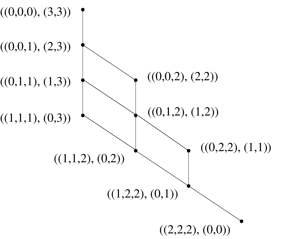
Step 2   The intermediate graph $\mathbf{\widetilde{\Gamma}(L_{1}\times L_{2})}$.

Let $\widetilde{\Gamma}(L_{1}\times L_{2})=\Gamma(L_{1})\Box\Gamma(L_{2})\Box\Gamma^{k,l}_{shuffle}.$ Label each vertex of $\widetilde{\Gamma}(L_{1}\times L_{2})$ with the ordered triple $(C_{1},C_{2},(\kappa,\lambda)),$ for all maximal chains $C_{i}\in L_{i},$ $i=1,2$ and for all possible shuffles $(\kappa,\lambda).$ The set of vertices of $\widetilde{\Gamma}(L_{1}\times L_{2})$ corresponds to all possible shuffles of pairs of maximal chains from $L_{1}$ and $L_{2}$, thus there is a one-to-one correspondence between the vertices of $\widetilde{\Gamma}(L_{1}\times L_{2})$ and the maximal chains of $L_{1}\times L_{2}$. From the definition of a cartesian product of graphs, two vertices in $\widetilde{\Gamma}(L_{1}\times L_{2})$, $(C_{1},C_{2},(\kappa,\lambda))$ and $(C^{\prime}_{1},C^{\prime}_{2},(\kappa^{\prime},\lambda^{\prime})),$ are adjacent if they satisfy precisely one of the following conditions:

1. (1)

   $C_{1}=C_{1}^{\prime}$, $C_{2}=C_{2}^{\prime}$, and $\kappa\sim\kappa^{\prime}$

2. (2)

   $C_{1}=C_{1}^{\prime}$, $C_{2}\sim C_{2}^{\prime}$ in $L_{2}$, and $\kappa=\kappa^{\prime}$

3. (3)

   $C_{1}\sim C_{1}^{\prime}$ in $L_{1}$, $C_{2}=C_{2}^{\prime}$, and $\kappa=\kappa^{\prime}.$

While $\widetilde{\Gamma}(L_{1}\times L_{2})$ has the right number of vertices, it has too many edges. For example, Figure 7 shows the possible result of shuffling $C_{1}$ with adjacent chains $C_{2}$ and $C_{2}^{\prime}.$ In one case, the shuffle results in a pair of adjacent chains in $L_{1}\times L_{2}$. However, using another shuffle results in chains that differ at three ranks in $L_{1}\times L_{2}$. This difficulty is easily remedied in Step 3 by removing a well-defined set of edges, determined by the rank where a pair of adjacent chains in one poset differs, along with the $k$- and $l$-sequences of the shuffle used.

Step 3   Removing edges from $\mathbf{\widetilde{\Gamma}(L_{1}\times L_{2})}$.

Each edge in $\widetilde{\Gamma}(L_{1}\times L_{2})$ can be classified as Type 1, 2, or 3, according to which of the above conditions is satisfied by $(C_{1},C_{2},(\kappa,\lambda))$ and $(C^{\prime}_{1},C^{\prime}_{2},(\kappa^{\prime},\lambda^{\prime})).$ The next step in the process of constructing $\Gamma(L_{1}\times L_{2})$ is to examine each type of edge in $\widetilde{\Gamma}(L_{1}\times L_{2}),$ to determine which ones are between a pair of adjacent chains in $L_{1}\times L_{2}$ and which are not. Once edges corresponding to pairs of non-adjacent chains have been removed from the graph, the result will be the desired final graph $\Gamma(L_{1}\times L_{2})$.

Type 1 edges. $C_{1}=C_{1}^{\prime}$, $C_{2}=C_{2}^{\prime}$, and $\kappa\sim\kappa^{\prime}.$ It is easy to see that none of these edges need to be removed. See Figure 5 for an example of this type.

Type 2 edges. $C_{1}=C_{1}^{\prime}$, $C_{2}\sim C_{2}^{\prime}$ in $L_{2}$, and $\kappa=\kappa^{\prime}.$ The diagram of $C_{2}$ and $C_{2}^{\prime}$ contains a diamond in $L_{2}$ at some rank $i$ where the two chains differ. When we shuffle $C_{2}$ and $C_{2}^{\prime}$ with $C_{1}$, this diamond may be stretched by the insertion of edges from $C_{1}$, depending on which shuffle is used. If $i\notin\kappa$ then the resulting chains are adjacent; but if $i\in\kappa$ then the resulting chains are not adjacent and the edge must be removed. Figure 7 shows the result of combining $C_{1}$ with both $C_{2}$ and $C_{2}^{\prime}$ using the shuffles associated with 3-sequences $(0,2,2)$ and $(0,1,1)$. Chains $C_{2}$ and $C_{2}^{\prime}$ differ at rank 1, but $(0,2,2)$ does not contain an element 1, so the shuffle does not stretch the diamond and the resulting chains are adjacent in $L_{1}\times L_{2}$. However, the shuffle associated with $(0,1,1)$ stretches the diamond by inserting two edges from $C_{1}$, so this Type 2 edge must be removed from $\widetilde{\Gamma}(L_{1}\times L_{2})$.

Type 3 edges. $C_{1}\sim C_{1}^{\prime}$ in $L_{1}$, $C_{2}=C_{2}^{\prime}$, and $\kappa=\kappa^{\prime}.$ As in the previous case, we must first identify the rank $i$ where $C_{1}$ and $C_{1}^{\prime}$ differ. If $i\in\lambda$ then the chains are not adjacent in $L_{1}\times L_{2}$ and the edge is removed from $\widetilde{\Gamma}(L_{1}\times L_{2})$.

This completes the determination of which edges to remove from $\widetilde{\Gamma}(L_{1}\times L_{2})$, resulting in the final graph $\Gamma(L_{1}\times L_{2})$.

While in [2], it was shown that for any connected graphs $\Gamma_{1}$ and $\Gamma_{2}$, we have that $A^{G}_{1}(\Gamma_{1}\Box\Gamma_{2})\cong A^{G}_{1}(\Gamma_{1})\times A^{G}_{1}(\Gamma_{2}),$ it is not immediately clear from the construction of $\Gamma(L_{1}\times L_{2})$ if there is an easily defined relationship between the groups $A^{G}_{1}(\Gamma(L_{1}))$, $A^{G}_{1}(\Gamma(L_{2}))$, and $A^{G}_{1}(\Gamma(L_{1}\times L_{2}))$. However, applying the construction defined in the previous section to $B_{n}$ leads to a better understanding of $\Gamma(B_{n})$ that allows us to use combinatorial methods to compute the abelianization of its $A_{1}$-group. We now reconstruct $\Gamma(B_{n})$ and characterize all of its primitive $6$-cycles.

In Figure 8, the vertices of $\Gamma(B_{3})$ and $\widetilde{\Gamma}(B_{4})$ are labeled with permutations written in one line notation. The graph $\Gamma(B_{1})$ consists of a single vertex, thus there are no Type 2 edges in $\widetilde{\Gamma}(B_{n})$ and we can simply consider the 1-sequences of $\Gamma^{3,1}_{shuffle}$. Labeling $\Gamma(B_{1})$ with the element 4 enables us to see the relationship between the 1-sequences labeling the shuffle graph and the position of 4 in the resulting permutations in $S_{4}$.

The graph in Figure 9 is another representation of the permutahedron we saw in Figure 3. The vertices are labeled with permutations of $S_{4}$, written in one line notation, and each edge corresponds to a (simple) transposition. $\Gamma(B_{4})$ illustrates the following (most of them well-known) properties of $\Gamma(B_{n}).$ All properties easily follow from the definition of the graph.

Properties of $\mathbf{\Gamma(B_{n})}$

1. (1)

   The graph $\Gamma(B_{n})$ is (n -1)-regular, with each vertex incident to precisely one edge for each of the $n-1$ transpositions $s_{i}\in\bf{S},$ $1\leq i\leq n-1.$ Label each edge with its associated transposition.

2. (2)

   Let level $i$ be the set of all permutations $\sigma\in S_{n}$ such that $\sigma^{-1}(n)=i.$ The graph has $n$ levels, and each level was initially a copy of $\Gamma(B_{n-1})$ before we removed edges from $\widetilde{\Gamma}(B_{n})$.

3. (3)

   The graph $\Gamma(B_{n})$ is bipartite, with vertices partitioned into even and odd permutations, and all cycles in the graph are of even length.

4. (4)

   The sequence of transpositions labeling the edges of a cycle in $\Gamma(B_{n})$ form a representation of the identity in $S_{n}$. Each 4-cycle in the graph corresponds to $(s_{k}s_{j})^{2}$ for some $1\leq k,\ j\leq n-1,$ where $|j-k|\geq 2.$ Each primitive 6-cycle corresponds to $(s_{j}s_{j+1})^{3}$ for some $1\leq j\leq n-2$.

Due to the structure of $S_{n}$, all other cycles of length $\geq 8$ can be expressed as the concatenation of 4- and 6-cycles; we can therefore limit our investigation to primitive 6-cycles. We want to count the $G$-homotopy equivalence classes of 6-cycles in $B_{n}$, which yields the rank of $A^{G}_{1}(\Gamma(B_{n}))^{ab}$. The following definition gives us an additional description of edges and cycles in $\Gamma(B_{n})$ that will help us determine equivalence classes of 6-cycles.

We note that all vertical edges between levels $i$ and $i+1$ are labeled with $s_{i}.$ We identify each vertical 6-cycle with the middle of its three levels. For example, 1243-2143-2413-4213-4123-1423 is a vertical 6-cycle at level 2 in $\Gamma(B_{4})$, and its edges are labeled with $s_{1}$ and $s_{2}$.

Let $C$ be a cycle in $\Gamma(B_{n-1})$. There are $n$ copies of $C$ in $\widetilde{\Gamma}(B_{n})$, one in each level of the graph. Each copy of $C$ in $\widetilde{\Gamma}(B_{n})$ is a horizontal cycle that is connected to the copies in neighboring levels by vertical edges, forming a net of vertical 4-cycles connecting all of the copies. For example, we see in Figure 8 that the 6-cycles forming levels 1 and 4 are connected by such a net. Removing vertical edges from $\widetilde{\Gamma}(B_{n})$ to form $\Gamma(B_{n})$ may remove edges from this net, however, it is easy to see that the copies of $C$ remain connected by a net of vertical 4- and 6-cycles, as seen in Figure 9.

In this section, we describe how to distinguish between different $G$-homotopy equivalence classes in $\Gamma(B_{n})$ so that we may count them. Specifically, we consider graph maps whose images in $\Gamma(B_{n})$ are primitive 6-cycles connected to the base vertex by a path, and we determine when they are $G$-homotopic to one another. We denote this relationship by $C_{1}\simeq_{G}C_{2}$, referring to the 6-cycles in the images rather than the graph maps themselves.

First, we show that if two 6-cycles are in the same equivalence class then they are associated with the same pair of transpositions, $s_{i}$ and $s_{i+1}$, for some $i$, $1\leq i\leq n-1$. We then prove a stronger theorem: 6-cycles $C_{1}$ and $C_{2}$ are in the same equivalence class if and only if they differ by a sequence of transpositions disjoint from $s_{i}$ and $s_{i+1}$. This theorem, when combined with our new understanding of the structure of $\Gamma(B_{n})$, gives us the means to describe the equivalence classes, and to find a formula for the rank of $A_{1}^{G}(\Gamma(B_{n}))^{ab}$.

Let $C_{1}$ and $C_{2}$ be distinct primitive 6-cycles in $\Gamma(B_{n})$. Let $\sigma_{0}$ be the base permutation and let $P_{1}$ and $P_{2}$ be paths from $\sigma_{0}$ to $C_{1}$ and $C_{2},$ respectively. Then by definition $C_{1}\simeq_{G}C_{2}$ if and only if there exists a $G$-homotopy grid such that the first row is $P_{1}C_{1}P_{1}^{-1}$ and the last row is $P_{2}C_{2}P_{2}^{-1}$.

Suppose that $C_{1}\simeq_{G}C_{2}$ and we have a $G$-homotopy grid from $P_{1}C_{1}P_{1}^{-1}$ to $P_{2}C_{2}P_{2}^{-1}$. We label each vertex in the grid with the corresponding permutation in $S_{n}$. Recall that a $G$-homotopy is itself a graph map that preserves adjacency, thus two vertices, $\sigma_{1}$ and $\sigma_{2}$, are adjacent in the grid if and only if $\sigma_{1}=\sigma_{2}$, or $\sigma_{2}=\sigma_{1}s_{i}$ for some $s_{i}$, $1\leq i\leq n-1$. If $\sigma_{2}=\sigma_{1}s_{i}$, then we label the edge with $s_{i}$; if $\sigma_{1}=\sigma_{2}$ the edge remains unlabeled. Each row in the grid is a loop based at $\sigma_{0}$, to which we associate a word in $S_{n}$ formed by the sequence of transpositions labeling the edges from left to right in the row. Let

We now consider the possible changes that we may make from one row to the next which preserve the $G$-homotopy relation, and describe each change in terms of operations on the associated words. Two graph maps are $G$-homotopic if they differ by 3- and 4-cycles, however, $\Gamma(B_{n})$ contains no 3-cycles. Furthermore, we saw in Figure 1 that it is not possible to contract a 4-cycle in a single step, thus the changes described below are the only permissible changes.

1. (T1)

   Repeating vertices. The $G$-homotopy relation is preserved by the repetition of a vertex in the image of a row, and the corresponding word does not change.

   

2. (T2)

   Traversing an edge in both directions. Traversing an edge once in each direction also preserves the $G$-homotopy relation and is equivalent to inserting $s_{i}^{2}$ into the associated word. Similarly, we may reverse this by removing such an edge, and deleting $s_{i}^{2}$ from the word.

   

3. (T3)

   Exchanging pairs of edges of a 4-cycle. Since 4-cycles are $G$-homotopic to the identity, we can replace two consecutive edges of a 4-cycle with the other two edges in the cycle. Recall that a 4-cycle is associated with $s_{j}$ and $s_{k}$, with $|j-k|\geq 2$. We see that the effect of this change is to commute $s_{j}$ and $s_{k}$ in the word. See Figure 13.

   

A key feature of each of the changes described above is that they preserve the parity of the number of transpositions $s_{i}$ (for each $1\leq i\leq n-1$) in the associated words. We also note that these changes do not include the use of the relation $(s_{j}s_{j+1})^{3}=1$ because that would involve exchanging consecutive edges of a primitive 6-cycle with the remaining edges. This would obviously not preserve $G$-homotopy because any cycle of length $\geq 5$ is not contractible to a single vertex.

Note that the above two types of operations, $(\textbf{T2})$ and $(\textbf{T3})$ generate an equivalence relation on the set $\sigma_{0}\textbf{W}$ of (based) loop-words, where

Two based words $\sigma_{0}W$ and $\sigma_{0}W^{\prime}$ are equivalent, $\sigma_{0}W\sim\sigma_{0}W^{\prime},$ if one can be obtained from the other by a sequence of $(\textbf{T2})$ and $(\textbf{T3})$ operations. Furthermore, two 6-cycles based at $\sigma_{0}$, $C_{1}$ and $C_{2}$, are $G$-homotopic if and only if their corresponding words, $\sigma_{0}W_{1}$ and $\sigma_{0}W_{2}$ are equivalent. Therefore we can continue our investigation of equivalence classes of 6-cycles using the language of graphs or words interchangeably.

Association with the same pair of transpositions is a necessary condition for $G$-homotopy of 6-cycles, but it turns out not to be sufficient. For $1\leq i\leq 6,$ let $\sigma_{i}$ and $\gamma_{i}$ be the vertices of the cycles $C_{1}$ and $C_{2}$ respectively. Since $\Gamma(B_{n})$ is connected there exists a path from $C_{1}$ to $C_{2}.$ Let $\tau_{i}\in\bf{S}$ and let $\tau_{1},\tau_{2},\ldots\tau_{k}$ be a shortest path from $C_{1}$ to $C_{2}.$ Moreover, assume that $\gamma_{1}=\sigma_{1}\tau_{1}\tau_{2}\ldots\tau_{k},$ and that we go around the cycles $C_{1}$ and $C_{2}$ in the $s_{i}$ direction. That is, $\sigma_{2}=\sigma_{1}s_{i}$, $\sigma_{3}=\sigma_{1}s_{i}s_{i+1}$ and so on. Similarly $\gamma_{2}=\gamma_{1}s_{i},$ $\gamma_{3}=\gamma_{1}s_{i}s_{i+1},$ etc. With this notation in mind we have the following theorem.

References

- [1] E. Babson, H. Barcelo, M. de Longueville, R. Laubenbacher. Homotopy Theory for Graphs, To appear in J. of Algebraic Combinatorics, 12 pp. 2005.
- [2] H. Barcelo, X. Kramer, R. Laubenbacher, and C. Weaver, Foundations of a Connectivity Theory for Simplicial Complexes, Adv. Appl. Math., 26 (2001), 97-128.
- [3] H. Barcelo and R. Laubenbacher, Perspectives on -Homotopy and its Applications, Discrete Mathematics, 298: 39–61, 2005.
- [4] H. Barcelo and R. Laubenbacher, Graph Theoretic Tools for Dynamic Network Analysis, preprints, 2005.
- [5] A. Björner, personal communication.
- [6] A. Björner, Subspace arrangements, Proceedings of 1st European Congress of Mathematics, Vol. I (Paris, 1992) (Basel) (Prog. Math., ed.), vol.119, Birkhäuser, 1994, 321–370.
- [7] A. Björner and L. Lovász, Linear Decision Trees, Subspace Arrangements and Möbius Functions, J. Amer. Math. Soc., 7 (1994), 677-706.
- [8] A. Björner and M. Wachs, Shellable nonpure complexes and posets I, Trans. AMer. MAth. Soc. 348, 1299–1327, 1996.
- [9] A. Björner and V. Welker, The Homology of “k-Equal” Manifolds and Related Partition Lattices, Adv. Math., 110 (1995), 277-313.
- [10] A. Dochtermann Hom complexes and homotopy theory in the category of graphs, arXiv:math/0605275v2 [math.CO]
- [11] A. Dochtermann Homotopy groups of Hom complexes of graphs, arXiv:0705.2620v1 [math.CO]
- [12] L. Hanish, C. Martin, R. Fabes, H. Barcelo, W. Griffin, The Breadth of Peer Relationship Among Externalizing Preschoolers: An Illustration of the Q-Connectivity Method, preprint, 2006.
- [13] X. Kramer and R. Laubenbacher, Combinatorial Homotopy of Simplicial Complexes and Complex Information Networks, Applications of Computational Algebraic Geometry (D. Cox and B. Sturmfels, eds.), Proc. Sympos. in Appl. Math., American Mathematical Society, vol. 53, Providence, RI, 1998.
- [14] G. Malle, A Homotopy Theory for Graphs, Glasnik Matematicki, 18 (1983), 3-25.
- [15] S. Maurer, Matroid Basis Graphs. I, J. Combin. Theory (B), 14 (1973), 216-240.
- [16] S. Smith, A Discrete Homotopy Theory for Graphs, with Applications to Order Complexes of Lattices, Ph.D. thesis, Arizona State University, http://faculty.gvsu.edu/smithshe, 2004.
- [17] R. Stanley, Enumerative Combinatorics, Volume 1, Cambridge University Press, New York, 1986.
- [18] G. Ziegler, Lectures on Polytopes, Springer-Verlag, New York, 1995.