A conformal approach
to numerical calculations
of asymptotically flat spacetimes
Dissertation
von
Anıl Çolpan Zenginoğlu
eingereicht bei der
Mathematisch-Naturwissenschaftlichen Fakultät
der Universität Potsdam
durchgeführt in Golm am
Max Planck Institut für Gravitationsphysik
Albert Einstein Institut
unter der Betreuung von
Prof. Dr. Helmut Friedrich
Potsdam, Juni 2007
Acknowledgements
I thank my supervisor Helmut Friedrich for suggesting the field of research and for forming my speculations into arguments with his supportive remarks. His deep understanding ranging from the broad picture to the minute details of technical questions showed me the way in many problems. I am especially grateful for his support and trust in difficult times during my thesis.
I thank Sascha Husa for guiding me in my first steps in numerical relativity and for his motivation, encouragement and support.
There are many people that I would like to thank who, directly or indirectly, helped me to develop some of the ideas presented in this thesis. I thank especially to Robert Beig, Christiane Lechner, Béla Szilágyi and Jeffrey Winicour.
For their help with computational infrastructure that I used in my numerical experiments I would like to thank Thomas Radke, Christian Reisswig, Erik Schnetter and Jonathan Thornburg.
I thank my office mates Florian Beyer, Roger Bieli and Carsten Schneemann for the pleasant office atmosphere we shared. I thank Andres Acena, Markus Ansorg, Badri Krishnan, Mark Heinzle, Jennifer Seiler and Tilman Vogel for fruitful discussions.
The Max Planck Institute for Gravitational Physics has been an efficient working environment for me with all the facilities that a researcher can wish for. In that respect I would like to thank the people working on backstage: Our cleaning lady Frau Pappa for a warm ”Günaydin!” each morning, our librarians Elisabeth Schlenk and Anja Lehmann, our secretary Anne Lampe and the computer support.
To Oya Çolpan
and Talha Zenginoğlu
Preface
The main question that this thesis tries to answer is the following: How can we calculate numerically the gravitational field of isolated systems in an efficient way based upon a clear geometric framework?
Isolated systems in general relativity are models of self-gravitating astrophysical sources. Depending on the scales in consideration, these sources can be planets, stars, black holes and even galaxy clusters. It is not the source that makes a system isolated, but the behavior of its gravitational field far away from the source. The systems that we might consider isolated share the property that as we move away from the source, the gravitational field becomes weak. We model such systems by suitably attaching to the far-field zone an asymptotic region in which the spacetime becomes flat in a certain sense. These models are commonly referred to as asymptotically flat spacetimes.
In this idealization procedure, the details of the asymptotic behavior need to be decided upon in accordance with physical intuition and the equations describing the model, as we can not yet observe the precise behavior of asymptotic gravitational fields to test and modify our assumptions.
An elegant and powerful characterization of the asymptotic behavior of spacetimes can be given in terms of the conformal structure. Conformal techniques make use of an important interplay between physics, conformal geometry and the theory of partial differential equations in the study of Einstein equations. The conformal approach has been applied successfully in mathematical relativity to various problems concerned with the large scale structure of spacetimes.
To relate observations of gravitational radiation to properties of astrophysical sources, we need to understand spacetimes representing isolated systems arising from a large class of initial data that correspond to astrophysical configurations. As the Einstein equations can not be solved explicitly for interesting dynamical systems emitting gravitational radiation, we need to apply approximation schemes to make quantitative predictions that can be compared with observations. The post-Newtonian and perturbative schemes cover the weak field and low velocity limits. To make reliable predictions on highly dynamical strong fields, we need numerical simulations.
There are many open problems in numerical calculations of spacetimes. At least two of these problems, namely the treatment of the outer grid boundary and the interpretation of numerically generated spacetimes, are related to the asymptotic region. Applying conformal techniques to deal with these problems can lead to accurate and efficient codes that allow us to gain control over numerical approximations.
An important goal of this thesis is the development of a numerical code that would allow us to calculate entire, asymptotically flat, radiative solutions to the Einstein equations. With such a code we should be able to follow the maximal development of asymptotically flat initial data starting from a Cauchy surface reaching spatial infinity up to the region close to timelike infinity. The achievement of this goal seems to require different methods adapted to different asymptotic regions, i.e. spatial infinity, null infinity and timelike infinity. With this goal in mind, we will discuss two novel applications of conformal techniques to numerical simulations. These new methods share the important advantage that the representation of the conformal factor is known a priori in terms of grid coordinates. I will argue that this feature is very convenient, because it is crucial to have numerical access to and some control over the asymptotic region for accurate and efficient calculations of asymptotically flat spacetimes.
Organization
In the introduction we describe shortly the development of some basic notions in conformal geometry. We mention the controversy on the nature of gravitational radiation and then present the idea of conformal infinity introduced by Penrose that is widely used in mathematical relativity today. We discuss conditions for the feasibility of the conformal approach investigated by Friedrich. An overview of current methods in numerical relativity with respect to the treatment of the far-field region of asymptotically flat spacetimes is given to motivate the numerical application of conformal techniques further.
Chapter 2 concentrates on infinity in null directions, called null infinity. In 2.1 and 2.2 we investigate spacelike slices reaching null infinity, so-called hyperboloidal slices, and conformal compactification of the Minkowski and the extended Schwarzschild spacetimes. We see that one can prescribe the representation of a conformal factor in terms of a suitably chosen compactifying radial coordinate on spherically symmetric hyperboloidal slices such that null infinity is at a fixed spatial coordinate location.
In 2.3 and 2.4 we construct a method to numerically treat the hyperboloidal initial value problem including null infinity in the computational domain without making any symmetry assumptions. This method allows us to find solutions to the Einstein equations in coordinates in which null infinity is fixed to a spatial coordinate location. It is based on the general wave gauge that is commonly used in numerical relativity. It introduces a suitable coupling of the conformal and the coordinate gauge to guarantee certain geometric properties of null infinity with an appropriate choice of the gauge source functions for the coordinates. It requires the numerical calculation of formally singular terms arising from the conformal compactification.
In 2.5 we discuss numerical test results obtained with the suggested method in the special case of spherical symmetry on the example of the extended Schwarzschild spacetime. We use a simple choice of evolution variables and numerical boundary treatment. While our numerical setup does not allow us to do long time evolutions of the extended Schwarzschild spacetime, one can see that the method can be applied even with crude numerical techniques without the formally singular terms leading to an immediate blow-up of numerical errors at the outer boundary.
The chapter ends in 2.6 with an outlook on next steps to establish this new approach for simulating dynamical isolated systems, and a short discussion of its open problems and limitations.
In chapter 3 we include not just null infinity but also spatial infinity in the numerical domain which gives us direct access to the global structure of asymptotically flat spacetimes. The reduced general conformal field equations developed by Friedrich provide the only available system for the treatment of spatial infinity. The system is based on the conformal Gauss gauge that we study using numerical methods. In 3.1 we reproduce Friedrich’s construction of a conformal Gauss gauge in the Schwarzschild-Kruskal spacetime numerically covering the entire solution in a smooth way. Going beyond analytical studies we find out numerically that one can also cover the Kerr solution using conformal geodesics including null infinity, timelike infinity and the Cauchy horizon.
In 3.2 we discuss certain aspects of the reduced general conformal field equations relevant for their numerical implementation. In 3.3 we solve numerically the Cauchy problem for the equations in spherical symmetry with initial data from the Schwarzschild-Kruskal spacetime which gives us the first numerical calculation of an entire asymptotically flat black hole spacetime including timelike, null and spacelike infinity and the region close to the singularity.
In order to include dynamical gravitational fields into our discussion of spacetimes in a neighborhood of spatial infinity, we calculate in 3.4 asymptotically flat, axially symmetric initial data based on studies by Friedrich. The calculated initial data has the special property that its ADM-mass vanishes but its development has a non-vanishing radiation field. In 3.5 we develop this data on a three dimensional Cartesian grid using the reduced general conformal field equations such that spatial infinity is represented by the point at the origin of our Cartesian grid. We calculate a certain component of the Weyl tensor in a suitably adapted Newman-Penrose tetrad representing the radiation field at null infinity and show that it does not vanish along null infinity in accordance with expectation.
The Cartesian code can not be used to study spacetimes with non-vanishing ADM-mass. For a generalizable code we implement the regular finite initial value problem near spatial infinity formulated by Friedrich based on the reduced general conformal field equations in a gauge that allows us to represent spatial infinity as a cylinder. The cylinder at infinity imposes a certain geometry that requires a numerical code which can handle a spherical grid topology in a frame formalism. In 3.6 we discuss a numerical implementation of a frame-based evolution system using spherical grid topology in three spatial dimensions with overlapping grids.
In 3.7 we implement the regular finite initial value problem with the cylinder at spatial infinity. A difficulty caused by the degeneracy of the equations at the set where the cylinder at spatial infinity touches null infinity is dealt with by freezing the evolution in the unphysical domain by exploiting the a priori knowledge of the conformal factor in terms of initial data and grid coordinates. The chapter ends with a discussion of possible improvements of the code.
In chapter 4 I summarize the main results of the thesis and give an outlook for possible directions for future work. The chapter ends with remarks on the idea of conformal infinity.
In the appendix A we discuss the generation of causal diagrams.
Chapter 1 Introduction
This thesis is concerned with numerical studies of asymptotic fields of isolated systems. Conformal techniques play a fundamental role in the discussion of the asymptotic structure of spacetimes. To develop an intuitive understanding of conformal rescalings, I will refer to their application in cartography where their advantages and disadvantages can be addressed in a simple manner and describe the argumentation of Hermann Weyl to emphasize the role of the conformal structure of spacetimes in general relativity.
The historical controversy concerning the physical nature of gravitational radiation is especially demonstrative for being cautious about interpretations of coordinate dependent calculations in general relativity. I will indicate how an unambiguous formulation of gravitational radiation that uses conformal techniques has been achieved.
The Penrose conformal compactification technique will be discussed and results on its feasibility due to Friedrich will be described. It is a goal of this thesis to combine a rigorous treatment of the far-field region of asymptotically flat spacetimes with advantages of widely used numerical methods. To motivate this goal I will point out certain properties of common numerical methods with special emphasis on their treatment of the asymptotic region.
The introduction follows chronological lines because I believe that some of the current problems in numerical relativity have their counterparts in earlier problems that have been thoroughly discussed. We can learn from these discussions to avoid similar confusions. Naturally, the presentation is highly subjective and makes no claim of completeness.
1.1 Conformal geometry
A map that preserves local angles is called conformal. The first problem where conformal mappings played an important role, beside the trivial rescaling where the conformal factor is just a positive constant, was the problem of projecting the surface of a globe onto a plane. The stereographic projection, probably already known to the Egyptians, has been applied in the 2nd century BC by Hipparchus to represent the celestial sphere on an astrolabe. Ptolemy used the stereographic projection for his cartography, a field which historically saw the most influential application of conformal techniques [87]. The Mercator projection of the Earth constructed in the 16th century is also a conformal projection. It was devised for nautical charts with the property that all lines of constant compass direction are represented by straight segments, but its use was not only restricted to marine navigation. The Mercator projection was so influential that its wide use was subject to political controversies related to the distortion of scales in conformal maps [38].
The development of methods in cartography has paved the way for the discussion on geometry of curved surfaces by Lambert, Bolyai, Lobachevsky, Gauss, Riemann and others. Indeed, some of the basic terminology in differential geometry has its origin in cartography. Therefore, it does not surprise that certain problems of cartography are similar to certain problems of general relativity. For example, it is clear today that in cartography different map projections serve different purposes. There is no single map of the Earth that covers all requirements. Similarly, there is no best gauge choice for a spacetime in general relativity. Emphasis on different aspects and parts of the solution require different gauge choices as will be demonstrated in this thesis by studies of various representations of the Minkowski and the Schwarzschild-Kruskal spacetimes.
A key feature leading to the wide use of the Mercator projection is the fact that it is a conformal projection. As a consequence the projection keeps relative local directions -in the sense of local angles- invariant. Clearly, relative local directions are important for marine navigation. In general relativity, the fundamental important structure is the causal structure which is equivalent to the null cone structure as well as to the conformal structure. We will see in the next sections how this fact can be used to get access to the large scale structure of spacetimes and to describe gravitational radiation rigorously, in an unambiguous way.
The importance of conformal geometry in general relativity has been recognized already in 1918 by Hermann Weyl [146]. His motivation to study conformal rescalings of the metric has partly been philosophical [126]. He was disturbed by what he called an inconsistency due to which lengths of vectors at different points in Riemannian geometry can be directly compared with each other. Weyl observes in [146]: ”The metric allows the magnitudes of two vectors to be compared, not only at the same point, but at any two arbitrarily separated points.” To remove this remnant of non-local geometry (”Ferngeometrie”), he proposed to consider the conformal class of a spacetime.
Let be a four dimensional, smooth manifold and a Lorentzian metric. The conformal class of a spacetime is given by metrics related to by a conformal rescaling with a positive, point dependent conformal factor . A choice of the unit of measurement, i.e. the gauge, corresponds to the choice of a metric in the conformal class or equivalently to the choice of a point dependent conformal factor . As a consequence, in Weyl’s ”pure infinitesimal geometry” [147], the choice of the unit of measurement is subject to local variations. Weyl states in [146] that for the explicit representation of the spacetime in such a geometry we have to choose a coordinate system and at each point determine the conformal factor. Therefore each formula must have a double-invariance, namely invariance with respect to arbitrary smooth coordinate transformations and with respect to conformal rescalings of the metric. For applications of conformal techniques in this thesis, especially in chapter 2, a suitable coupling of the coordinate and the conformal gauge freedom will be essential to gain control over the asymptotic region.
The main step from Euclidean geometry to Riemannian geometry is the removal of the assumption of integrability of vectors by parallel transport. In Riemannian geometry, a vector parallel transported along a closed curve changes in general its direction due to curvature, while its norm stays the same. Weyl demanded “the non-integrability of the transference of distances” [150]. He states in [146]: ”A true infinitesimal geometry should, however, recognize only a principle for transferring the magnitude of a vector to an infinitesimally close point and then, on transfer to an arbitrarily distant point, the integrability of the magnitude of a vector is no more to be expected than the integrability of its direction.” To allow for comparison of lengths in each small neighborhood, he introduced what we call today the Weyl connection. A concise description of these ideas can be found for example in [1, 105]. We use a modern representation following the notation of [64].
A Weyl connection is a torsion free connection which is not necessarily the Levi-Civita connection of a metric in the conformal class but preserves the conformal structure so that the covariant derivative of any metric in is proportional to itself,
| (1.1) |
with a one-form . Under conformal transformations of the metric with a function , the one-form transforms according to . If is exact, it can be written as and the Weyl connection is the Levi-Civita connection of a metric in the conformal class given by .
The relation of the Weyl connection with a metric connection of a metric in the conformal class is given by
| (1.2) |
We see that Weyl connections characterized by 1-forms allow us a more general discussion of the conformal structure than conformal rescalings of the metric.
The introduction of the Weyl connection was the first step in the study of generalized connections and it led to a rich geometry, which Weyl used in his attempt to unify the gravitational and electromagnetic fields. His attempt for a unified theory was unsuccessful due to physical observations [76], however the main idea has been the basis during the construction of modern gauge theories [101]. It is interesting to note that the concept of gauge invariance in theoretical physics originates in Weyl’s ideas on conformal invariance [102].
A torsion free connection implies the notion of parallel transport and allows the construction of geodesics. Auto-parallel curves with respect to a Weyl connection are referred to as conformal geodesics [70]. Remarkably, conformal geodesics have been useful in investigations of the asymptotic behavior of solutions to Einstein equations carried out by Helmut Friedrich [64]. Following his investigations, we will make use of conformal geodesics in chapter 3 for a numerical treatment of spatial infinity.
The application of conformal techniques in general relativity played an important role in the clarification of a heated controversy in mathematical relativity on the physical nature of gravitational radiation that we discuss in the next section.
1.2 Gravitational radiation and asymptotic flatness
The Newtonian theory of gravitation is governed by a linear elliptic Poisson equation for the Newtonian potential and does not allow for free gravitational degrees of freedom carrying energy. The action-at-a-distance property of Newtonian gravitation related to the elliptic nature of the underlying Poisson equation was already questionable to Newton and his contemporaries. A finite speed of gravity has been studied by Laplace who concluded from this assumption to a damping force on the orbital motion of planetary systems. In 1908, Poincaré suggested an acceleration of planetary orbits due to loss of energy by emission of gravitational waves.
The first relativistic description of gravitational waves is due to Albert Einstein [46, 47]. He studied wave phenomena in linearized gravity and introduced the quadrupole formula which, in the weak field limit, relates the motion of a source to generation of gravitational waves. In his linearized calculations he made use of a coordinate dependent quantity which he called the pseudo energy momentum tensor to calculate the energy flux of gravitational waves. Einstein’s use of the coordinate dependent pseudo-tensor was criticized by many scientists of his time [31], among others Eddington who suggested to put more emphasis on the curvature tensor, showed that certain classes of wave-like solutions to the linearized Einstein equations are not physical and pointed out limitations of linearized calculations [45].
Until the 1960s the status of gravitational waves was quite uncertain. Even Einstein seems to have believed for some time that gravitational waves did not exist [86]. The use of linearized calculations whose qualitative predictions are not necessarily valid in the full theory, the application of coordinate-dependent methods and the non-local nature of gravitational field energy have been sources of confusion. The difficulty with a local energy concept for the gravitational field lies in the background independence of general relativity. Due to the equivalence principle, the local gravitational field can be transformed away by passing to a freely falling frame of reference.
With the work of Lichnerowicz on mathematical foundations of general relativity [94] it turned out that certain calculations supporting the view that gravitational waves are unphysical put too restrictive conditions on coordinates. Based on the development of mathematical foundations and a stronger emphasis on curvature invariants, the question on the status of gravitational waves was gradually answered by the works of Bondi, Newman, Penrose, Petrov, Pirani, Robinson, Sachs and Trautman among others.
It is difficult to give a precise definition to radiation in general relativity as the gravitational field acts as its own source so that there is no background we can rely on. However, the gravitational field becomes weak far away from sources. When we concentrate our studies on an astrophysical system we assume that the interaction of this system with the rest of the universe to be negligible. In the study of such ”isolated systems” the astrophysical system is modeled by an asymptotically flat spacetime. This corresponds to an idealized situation in which massive sources are confined to spatially compact domains and the spacetime metric is required to approach a flat metric at infinity. One might hope to find a precise notion of radiation for such systems in the asymptotic region using the flat limit metric as a kind of background structure.
For the discussion of gravitational radiation, it is natural to require asymptotic flatness in null directions. Historically, however, first discussions of asymptotic flatness have been made with respect to spatial infinity. Note that asymptotic flatness is an assumption that is ”put in by hand”. Today there are several mathematically inequivalent definitions of the concept and we will refer to some of them in later sections. In essence, one imposes some condition determining the approach of the metric to a flat metric at (spatial or null) infinity. A formal definition based on the existence of distinguished classes of coordinates, say near spatial infinity, can be roughly given as follows. We may call a spacetime asymptotically flat at spatial infinity when there exists a coordinate system in a neighborhood of spatial infinity with respect to which
| (1.3) |
where with . We denote by the Minkowski metric, is the Kronecker symbol and the terms behave like under differentiations of order . The strength of the fall-off behavior is determined when we give a precise description of . A question is how strong this fall-off behavior needs to be so that suitable physical notions of total energy, linear and angular momentum can be defined. It is known, for example, that for and a well-defined notion of total energy at spatial infinity can be associated with an asymptotically flat spacetime [130].
The linearized theory suggests that gravitational perturbations travel along null directions. Therefore, to define gravitational radiation, one takes limits to infinity in null directions. One may define a notion of asymptotic flatness in null directions by requiring (1.3) in a neighborhood of null infinity with respect to a suitable coordinate system. We might intuitively imagine that the spacetime should become simply close to the Minkowski spacetime in whatever direction we approach infinity. The geometric picture, however, is quite different and it is a delicate question how the notions of asymptotic flatness at spatial and null infinity fit together. We will come back to this issue at the end of the section. Let us first follow the historical development of the concept of gravitational radiation.
An important step in the clarification of questions regarding gravitational radiation was the demonstration that outgoing gravitational radiation carries positive energy away from an isolated system [21, 120]. This analysis used a special class of coordinate systems which is natural for studying radiation phenomena. The coordinates are generated by distinguished families of outgoing null hypersurfaces. On the hypersurfaces the luminosity distance has been defined. Today such coordinates are called Bondi coordinates. The field equations have been studied along null directions and certain conditions at infinity have been put that are similar to the no incoming radiation conditions suggested by Trautman [138]. These conditions included the requirement that metric components have certain smoothness properties in in the limit along null directions. An important open problem was whether and to what extend these conditions excluded interesting solutions [120].
Instead of putting conditions on metric components corresponding to asymptotic flatness as above, it is more convenient to impose restrictions on certain components of the Weyl tensor representing the free gravitational field. Sachs analyzed the vacuum Bianchi identities and suggested that the Weyl tensor satisfies a ”peeling property” along outgoing null geodesics relating the fall-off behavior of its components to the Petrov classification [119]. Shortly after this analysis, Newman and Penrose found a way to formulate fall-off conditions in an elegant way and showed that they imply the peeling behavior [100]. They introduced the spin frame formalism and analyzed expansions of gravitational fields in where is an affine parameter along outgoing null geodesics. Imposing a certain uniform smoothness condition, they found out that if a particular complex tetrad component of the Weyl tensor with respect to a distinguished tetrad at infinity has an asymptotic behavior and as , one can derive the Sachs peeling behavior as for . In analogy to electromagnetism, the field with the weakest fall-off in the order , namely , is interpreted as representing the outgoing radiation field. Note that this interpretation of is strongly related to the Sachs peeling behavior and requires a distinguished choice of a tetrad field at infinity. In contrast to electromagnetism, where the linearity of the Maxwell’s equations allows a clean global separation between near field terms and far field terms, in general relativity no such separation can be expected in general as the peeling behavior is valid only in the asymptotic region. In the strong field regime one would expect a mixture of the fall-off behavior. Therefore it is misleading to talk about calculated with respect to some tetrad field in the interior as the radiation field.
In the studies just discussed, the close relationship between gravitational radiation and asymptotic behavior of solutions to the Einstein equations has been demonstrated. However, the studies still relied on the use of special classes of coordinate systems and included awkward limits to infinity. Such limits arise because a rigorous meaning to gravitational radiation can only be given in the asymptotic region.
To study physical properties of isolated systems, one would like to have coordinate independent definitions. The coordinate dependence in the early studies of gravitational radiation blurred the global geometric structure of asymptotically flat spacetimes. In the early development of the field, the global picture was by no means clear, not even to those who contributed substantially to the development of the picture. Sachs, for example, refers to null infinity as ”the cylinder at spatial infinity” in [120].
To motivate a coordinate independent approach to the concept of gravitational radiation further and to point out a subtlety regarding the notion of asymptotic flatness in spacelike and null directions, we shall discuss an illustrative example taken from [110]. The Schwarzschild metric with mass in standard Schwarzschild coordinates reads
| (1.4) |
where . This metric obviously approaches the flat Minkowski metric given by , as , so that we may call the Schwarzschild spacetime asymptotically flat at spatial infinity. This, however, does not by itself imply that the Schwarzschild spacetime is asymptotically flat in null directions. With regard to null geodesics the Schwarzschild metric (1.4) differs greatly from the Minkowski metric at large distances. Consider outgoing null geodesics given by , , , where is the Schwarzschild retarded time . We see that as the value of the Minkowski retarded time is unbounded above along outgoing Schwarzschild null geodesics (the argument applies also for ingoing null geodesics). Schwarzschild null geodesics do not correspond at all to Minkowski null geodesics with respect to for large .
The solution to this apparent problem is to relate a Minkowski metric to the Schwarzschild metric in a different way. Define a coordinate . We can choose on the Schwarzschild manifold another Minkowski metric given by . Now the described difficulty does not arise because outgoing null geodesics given by have the same form for both metrics and . While the condition for asymptotic flatness (1.3) has the same form in spacelike and null directions, its geometric interpretation, i.e. the way we relate the Minkowski metric to the curved spacetime metric , is different.
We mentioned that for studying gravitational radiation one might use the flat limit metric as a kind of background structure. This example makes clear that the relation of the flat limit metric to the curved spacetime is determined by the null cone structure. The null cone structure, however, is part of the unknown in the Einstein equations. It is therefore a difficult question how the flat background structure can be used conveniently in dynamical spacetimes to discuss their asymptotic properties.
It turns out that the structure that we are looking for can be given in terms of the idea of conformal infinity presented in the next section. This construction also allows to replace asymptotic calculations by local differential geometry.
1.3 Conformal infinity
Conformal techniques in general relativity played an important role in the investigation of the solution space to the Einstein equations. The analysis of elliptic constraint equations implied by the Einstein equations on spacelike hypersurfaces has made intensive use of conformal methods [93, 153]. In the following, we will concentrate on conformal rescalings of the full spacetime metric. We will also ignore the application of conformal techniques in cosmological models (see [60] for an overview and [17] for a recent work).
It was discovered by Penrose that a suitable notion of asymptotic flatness can be formulated in an elegant way using the conformal equivalence class of the metric. The conformal compactification technique enabled a geometric formulation of the fall-off behaviour. Penrose could also deduce the peeling behavior from a few assumptions on the conformal structure of the metric not favoring any coordinate systems [107, 108]. Since then, conformal techniques to study in detail the structure of gravitational fields in the asymptotic region in a coordinate independent way have been very fruitful in mathematical relativity. Many physical concepts like mass, momentum or gravitational radiation of isolated systems have been unambiguously defined in the asymptotic region of an isolated system using conformal techniques.
Two important observations suggest a conformal approach for discussing radiation. The first observation is the importance of the null cone structure. Conformal rescalings of the metric preserve the null cone structure, which is equivalent to the characteristic and the causal structures. It turns out that essential features of free gravitational fields strongly related to the null cone structure can be discussed with respect to the conformal equivalence class of the physical metric. The second observation is related to the non-local feature of gravitational radiation which requires limits to infinity as discussed in the previous section. Conformal rescalings can be used to avoid such limits by compactifying the spacetime such that infinity corresponds to a finite hypersurface. Asymptotic calculations can then be replaced by local differential methods under certain conditions.
The idea of conformal compactification is similar to the construction of the Riemann sphere in complex analysis by adjoining infinity to the complex plane. Due to the Lorentzian signature of the metric, infinity for a spacetime corresponds not to a point but has a richer structure, as Weyl already observed in [148]. To demonstrate the technique we discuss the conformal compactification of the Minkowski spacetime (see also [51, 109, 144]).
The Minkowski metric in coordinates adapted to spherical symmetry is given by
| (1.5) |
where is the standard metric on the unit sphere . Introducing null coordinates and for , and compactifying them by and , we get
Points at infinity with respect to the original coordinates have finite values with respect to the compactifying coordinates ( or ), however, the physical metric in compactifying coordinates is singular at these points. This singular behavior can be compensated by a conformal rescaling with the conformal factor , so that the rescaled metric
is well defined on the domain including points that are at infinity with respect to . We say that can be extended beyond infinity.
For Fig. 1.1 time and space coordinates and have been introduced. The resulting metric is the standard metric on the Einstein cosmos . The embedding of the Minkowski spacetime into the Einstein cosmos is given by
from into , , suppressing the angular coordinates. The part of that corresponds to the Minkowski spacetime is given by .
We see that the completion of is a manifold with boundary , where the boundary points correspond to points at infinity with respect to the physical metric. Asymptotic behavior of fields on can be studied using local differential geometry on this boundary where the conformal factor vanishes. The part of the boundary without the points at is denoted by . The differential of the conformal factor does not vanish at , , and consists of two parts , each of them with the topology .

Fig. 1.1 shows curves that correspond to constant values of the coordinates and in the new representation. Each point of the diagram represents a sphere except the dashed vertical line segment connecting and which corresponds to the origin . Surfaces of approach timelike infinity , surfaces of approach spatial infinity . The figure is a Penrose diagram which is especially useful for depicting causal structures. In Penrose diagrams, radial light rays are straight line segments with 45 degrees to the horizontal. Null rays ( and surfaces) reach for an infinite value of the physical affine parameter along them, hence is called null infinity.
The idea is now to take certain properties of the asymptotic structure of the Minkowski spacetime as being representative for the asymptotic structure of isolated systems. We make the following assumptions about an asymptotically flat spacetime : There exists a regular spacetime , a sufficiently differentiable (say ) function on and an embedding , which is conformal with conformal factor such that The conformal factor satisfies on and the completion of is a submanifold with non-empty boundary , that is , on which . These assumptions are closely related to the notion of weak asymptotic simplicity [108]. In the following, we identify with so that we write or . The triple is called conformal extension of . Note that the conformal extension is not unique.
The basic assumption here is that the rescaled metric is regular across . A similar construction where this assumption is satisfied can be made for other explicit solutions that can be regarded as asymptotically flat, for example the Schwarzschild-Kruskal solution (see Fig. 1.2 for the resulting Penrose diagram). However, we do not have a large class of explicit radiative solutions where we can test our requirements on the conformal extension. Therefore we do not know whether the above assumptions cover sufficiently general spacetimes so that we can take a conformal approach in the isolated system idealization of interesting astrophysical configurations .
A strong support for the conformal compactification technique comes from the studies described in the previous section. Results achieved by coordinate dependent methods and limits to infinity can be derived very elegantly for spacetimes admitting a smooth conformal boundary using the conformal technique [107, 108].
To utilize the conformal compactification technique for calculating gravitational radiation we would like to answer: How general is the description proposed by Penrose? [111]

The details of the conformal compactification technique have been motivated by explicit examples or well studied assumptions about the fall-off behavior of certain fields as above and not by a detailed study of the full non-linear Einstein equations. The assumption on smoothness of is geometrical and includes only requirements on the conformal class . Smoothness of the rescaled metric along the conformal boundary corresponds to a fall-off behavior for the physical metric , which is however a solution to the Einstein equations that impose their own asymptotic behavior. It might be that the smoothness requirement on the conformal extension is too restrictive such that only a very special class of solutions satisfies it. Whether the geometrical requirement of smoothness of is compatible with the fall-off behavior of the metric fields as a solution to the Einstein equations is a delicate question.
We would like to know by some general argument whether we have a large class of non-trivial, asymptotically flat, radiative spacetimes that admit a smooth conformal boundary such that we can apply the conformal compactification technique. To answer this question, the solution space to the Einstein equations needs to be studied with an emphasis on the asymptotic structure of gravitational fields.
The available explicit solutions are not general enough to study the solution space by direct means, therefore we are led to abstract analysis. By sufficient knowledge on properties of spacetimes, we can get some results in certain classes. We know, for example, that asymptotically flat, vacuum, stationary spacetimes admit an analytic compactification at null infinity [42]. For more general results that include radiative spacetimes, the initial value problem needs to be studied in a general setting.
The analysis of the initial value problem for Einstein equations in the compactified picture is not straightforward, as the Einstein equations are not conformally invariant and compactification leads to formally singular equations at infinity. However, the equations are conformally regular as Friedrich showed by constructing a system which is equivalent to the Einstein equations for and is regular for all values of the conformal factor so that the equations for the rescaled metric can be analyzed on a conformal extension including where [53].
Friedrich analyzed the initial value problem for the conformally regular field equations based on spacelike surfaces that extend smoothly through null infinity. These surfaces are called hyperboloidal as their asymptotic behavior is similar to the standard hyperboloids in Minkowski spacetime [54]. Let be such a hyperboloidal surface that cuts in a spacelike two dimensional surface and extends smoothly through as in Fig. 1.3 (the discussion of follows by time reversal). The analysis of the hyperboloidal initial value problem revealed that if regular data for the conformally regular field equations is given on , the smoothness of will be preserved into the future of , at least for a while [54]. While this result is local in time, Friedrich also proved a semi-global stability result stating that, for small data, will admit future complete null generators and a regular timelike infinity [56]. The existence of regular data for the conformally regular field equations has been shown in [3]. The analysis of [3] showed further that, in general, even with the strongest smoothness requirements on free data, logarithmic singularities can arise at unless some mild regularity conditions on the geometry of are satisfied.

These analytic results are important for practical purposes in numerical calculations. One should be aware that the requirement of the existence of a smooth implies a restriction on the data. One may expect that this restriction does not exclude physically relevant solutions, but this is yet an unresolved question. Still, for a non-smooth some of the relevant structure may be recovered [35, 151]. It is an interesting open question whether one can deal with some mildly singular behavior numerically. We will study the hyperboloidal initial value problem in chapter 2.
The analytic results just described show that the decision on smoothness of null infinity is made at spatial infinity . Remarkably, our knowledge on the asymptotic behavior of solutions like Schwarzschild or Kerr can be applied to this question. By gluing techniques developed by Corvino and Schoen [36], one knows that there exists a large class of non-trivial initial data which is Schwarzschild or Kerr in a neighborhood of spatial infinity. As stationary spacetimes admit an analytic compactification at null infinity, we know that the development of such data leads to regular hyperboloidal initial data. Combined with Friedrich’s results on the hyperboloidal initial value problem this leads to the existence of a large class of non-trivial, radiative, vacuum spacetimes with smooth null infinity [34]. These spacetimes, however, have a special asymptotic structure. The question still remains whether more general spacetimes exist. To answer it, the behavior of gravitational fields in a neighborhood of spatial infinity needs to be studied in detail.
A detailed study of solutions in a neighborhood of spatial infinity is complicated by the fact that when the ADM-mass of the spacetime does not vanish point compactification at spatial infinity leads to a certain singular behavior. Physical fields do not admit smooth limits at the point . The limits depend on the spacelike direction along which one approaches [75, 4]. Therefore, to study fields at spatial infinity, it might be better not to represent it as a point. In [5, 14, 127], a representation of spatial infinity as a unit timelike hyperboloid has been used. This representation of spatial infinity, however, does not allow a study of the full system of the Einstein equations in a unified picture with spatial and null infinity.
A regular finite initial value problem near spatial infinity has been formulated by Friedrich using the reduced general conformal field equations that he introduced in [58]. These equations are written in a conformal Gauss gauge based on conformal geodesics which are auto-parallel curves with respect to a Weyl connection [63, 70]. In the conformal Gauss gauge, spatial infinity can be represented as a cylinder. The cylinder at infinity allows a detailed discussion of gravitational fields at spatial and null infinity in a single, regular setting that only depends on the conformal structure of the spacetime [61, 64].
Friedrich’s analysis showed that in general, logarithmic singularities arise in a small neighborhood of spatial infinity. He obtained necessary regularity conditions on the Cotton tensor for these singularities to vanish. Later on, Valiente Kroon showed that these conditions are not sufficient and obtained further obstructions to smoothness of null infinity [141]. The question on necessary and sufficient conditions on Cauchy data for smoothness of is still open and a field of active research. A rich structure can be expected in a neighborhood of spatial infinity, as suggested for example by the existence of initial data whose development may lead to different smoothness properties on past and future null infinity [142].
For having numerical access to spatial and null infinity in a single setting, the reduced general conformal field equations are the only tool we have at present. A numerical implementation of this system needs to deal with certain difficulties. The regular finite initial value problem at spatial infinity distinguishes directions at spatial infinity. The regular representation of conformal data on a Cauchy surface crucially relies on a conformal rescaling of a distinguished tetrad with respect to which the fields are calculated. For numerical studies using this system, the geometry imposed by the cylinder needs to be implemented. We will discuss an implementation and tests in chapter 3.
In this section, I described conformal techniques and some analytic results on their applicability to present the analytic foundation on which the numerical studies of this thesis are build. The studies are complementary to existing numerical methods but they are not an aim by themselves. A motivation to use conformal techniques in numerical calculations is given by the hope that interaction between mathematical and numerical methods will lead to fruitful studies of the solution space to the Einstein equations. Especially interesting seems the question, whether a mildly singular behavior of solutions at infinity can be treated by numerical methods so that conjectures on properties of solutions can be made which in turn might be studied by rigorous analyses.
Another basic motivation is achieving efficient numerical simulations of isolated systems using controlled approximations so that reliable predictions on gravitational radiation can be made. Current numerical methods to calculate gravitational radiation have certain disadvantages that we will discuss in the next section to give an overview on the subject and to put the conformal approach in numerical relativity into its broader context.
1.4 The outer boundary in numerical relativity
To study the development of large classes of data and to make quantitative predictions on highly dynamical, strong gravitational fields, we need to use numerical methods. The Einstein equations written in arbitrary coordinates are of no known type as they only determine the isometry class of the metric. To numerically calculate a solution metric with given initial data on some hypersurface, one typically reduces the Einstein equations to a hyperbolic system of partial differential equations. The reduced system is discretized and solved iteratively by some numerical algorithm. A reduction can be done in various ways which suggests a variety of methods in numerical relativity.
Special properties of general relativity among other theories of physics, particularly the lack of a background and related difficulties like the non-linearity of the equations or the non-local feature of gravitational field energy, require a strong interplay between mathematical and numerical methods not only on numerical analysis or analysis of partial differential equations, but also on differential geometry. The importance of abstract methods that can suggest well-defined techniques for numerical calculations has been recognized only recently. Today, the numerical stability problem for some astrophysically interesting classes of data seems to be solved. The numerical development of various binary black hole initial data, which was a big challenge for many years, can now be followed from the late inspiral through the coalescence phase [10, 23, 30, 89, 113, 122, 131].
There remain, however, many open problems that need to be studied. In this thesis we are mainly concerned with numerical studies of the asymptotic behavior of isolated systems. We will therefore concentrate on problems concerning the numerical treatment of the asymptotic region. To illustrate the computational domain in various methods that we discuss, the regions I and II in the Penrose diagram of the Schwarzschild-Kruskal spacetime from Fig. 1.2 will be plotted. We will also discuss the causal structure on the grid depicted by ingoing and outgoing null surfaces. We will assume that the interior of the event horizon is dealt with by the excision method. This corresponds to the introduction of a spacelike boundary inside the black hole so that no boundary data needs to be given. The requirement for the numerical treatment of such a spacelike inner boundary is numerical stability. There are other possibilities for treating the singularity that we ignore.
1.4.1 Timelike artificial boundary
The asymptotic region of isolated systems extends to infinity. To simulate such spacetimes numerically on a finite grid, the most common method truncates the computational domain by introducing an artificial, timelike outer boundary which introduces certain problems that we discuss in the following. Fig. 1.5 shows a typical foliation of the Schwarzschild-Kruskal spacetime along with timelike surfaces that may act as artificial boundaries. The diagram has been calculated using the ingoing Eddington-Finkelstein coordinates described in Appendix A.
The introduction of an artificial, timelike, outer boundary implies an initial boundary value problem for a hyperbolic reduction of the Einstein equations which should be well-posed. The requirement of well-posedness is not just a mathematical subtlety but is also physically motivated. It means that unique solutions are required to exist that depend continuously on initial data. This is strongly related to the requirement of predictability on a physical theory.
Further, the solutions to the reduced system should correspond to solutions to the full system in the sense that the vanishing of the constraints on an initial hypersurface is preserved into the future of that surface. Therefore, the boundary conditions at the outer boundary should preserve the vanishing of the constraints. Such a well-posed, constraint preserving initial boundary value problem for Einstein equations has been constructed by Friedrich and Nagy [68]. Their frame-based, first order formulation allows the adaptation of the evolution system to a timelike outer boundary such that the constraints are propagated by maximally dissipative boundary conditions without the need to restrict the boundary data. However, their reduction has not yet been used in numerical simulations. Currently, there are many studies on the the initial boundary value problem for the Einstein equations using methods that are simpler to implement in numerical calculations but do not solve the full problem [6, 7, 88, 91, 117, 118, 121].


Another difficulty concerns the choice of boundary data. We see in Fig. 1.5 that ingoing characteristics enter the spacetime from the outer boundary. One might wish to prescribe data on these characteristics that would correspond to a no incoming radiation condition. However, the timelike outer boundary surface is geometrically arbitrary, without invariant meaning. Apart from the problem related to its gauge dependent choice, it seems difficult to give a precise definition of gravitational radiation on such a surface. This difficulty is related to the lack of a quasi-local energy concept in general relativity. Besides, such a no incoming radiation condition will not in general correspond to the transparency of the artificial boundary due to backscattering of gravitational radiation, which is related to the non-linearity of the theory. To give an example for potential problems, we mention that it has been proven that certain types of commonly used boundary conditions in numerical relativity destroy the tail behavior [40]. Nonetheless, there are detailed analyses on how to deal with these problems in the linearized regime [26, 27].
The problems described above can be treated numerically provided that the outer boundary is sufficiently far away so that linearized analysis is a good approximation. When the outer boundary is far enough, a numerically stable treatment might be good enough as one can trust the solution up to numerical accuracy on the domain of dependence of the initial hypersurface. As can be seen in Fig. 1.5, the domain of dependence grows when the outer boundary is put farther away. A difficulty arises due to the slow fall-off rate of the radiation field. To gain a factor of in accuracy, the outer boundary needs to be pushed to twice the distance which requires times the number of grid points on a homogeneous grid in a simulation in three space dimensions. Therefore, today’s numerical codes use inhomogeneous grids. By using mesh refinement techniques one can put the outer boundary to as far as [9, 97]. Mesh boundaries, however, cause numerical errors and there is still a problem of efficiency on foliations that approach spatial infinity with increasing physical distance. Such foliations waste computational resources, as one needs long time evolutions to calculate the emission of radiation in the far-field zone.
This brings us to the radiation extraction problem. In the analysis of numerically generated spacetimes, one calculates certain quantities interpreted as gravitational radiation along a timelike surface representing a family of observers far away from the source whereas is the natural place to measure emission [50]. As there is no unambiguous definition of gravitational radiation at a finite distance away from the source one uses approximative methods. A common method, called the Regge-Wheeler-Zerilli method assumes that the full metric in the extraction region is a perturbation of the Schwarzschild spacetime in a certain gauge and tries to extract radiation information in a coordinate invariant way [115, 156]. Another method relies on calculating Weyl scalars with respect to a special tetrad class, called the quasi-Kinnersley frame, that can be constructed in an invariant way in spacetimes of Petrov type D [99]. These methods rely on linearized approximations. As shown in [106], different extraction methods can deliver different results in an accurate code so that numerical error is dominated by systematic error from the extraction method. Note that this error can not be estimated by convergence tests. Even in the continuum limit of infinite resolution, the calculation of gravitational radiation will have the same systematic error.
To estimate the extraction error, one can put the extraction surface farther away so that the systematic error decreases typically with . However, there are limitations on the choice of the observer location that also limit the accuracy of radiation extraction. On the one hand, one should not put the observer too close to the sources because the assumptions underlying the extraction method are not valid in the strong field regime. On the other hand, one should not put the observer too far, because then the contamination from the outer boundary hits the extraction surface before the waves reach the observer. A further difficulty arising from putting the extraction surface far away is due to numerical dissipation which lowers the accuracy of the extraction as the waves propagate slowly along the grid. Today, the observer location for wave extraction is typically set to about [16, 97].
Although recent years saw quite impressive advances in the problems mentioned, one can say that there is still a lack of appreciation of global or semi-global considerations. While the problems we alluded to can be regarded as subtleties and not crucial for the detection of gravitational waves, the approximation errors might turn out to be relevant for gravitational wave astronomy where accurate waveforms are needed that might in principle allow us to decide on different equations of state for inspiralling neutron stars or to extract the remnant gravitational radiation from the big bang. Such questions require accurate predictions under controllable approximations. As large parameter studies need to be done, the efficiency of the codes will also play an important role.
Beside the requirement of an unambiguous radiation extraction we can deduce the following requirements on a smooth foliation for a clean boundary treatment just by considering the causal structure on the grid as depicted in Fig. 1.5:
- •
No characteristics should enter the computational domain from the boundary.
- •
Outgoing characteristics should leave the computational domain through the boundary.
Note that both requirements are fulfilled for excision along a spacelike inner boundary inside the black hole.
In the following we will review alternative methods that have been suggested to deal with the problems of the artificial timelike outer boundary approach.
1.4.2 Coordinate compactification at spatial infinity
To avoid problems related to the treatment of the outer boundary within the standard 3+1 approach, one can use a compactifying coordinate system on the Cauchy hypersurfaces. Then the outer boundary of the computational domain is at spatial infinity where natural boundary conditions can be used [33, 113].
To elucidate the idea, take an asymptotically flat, two dimensional spacetime metric and a time function such that surfaces are Cauchy surfaces. Introduce on these surfaces a coordinate . We write the metric on the coordinate domain as
To avoid a timelike outer boundary, we can introduce a compactifying coordinate by setting . The coordinate transformed metric takes the form
| (1.6) |
The coordinate value corresponds to spatial infinity as the surfaces are Cauchy surfaces. While the transformed metric components and are singular at this point, the untransformed ones attain their Minkowski values for an asymptotically flat spacetime. A numerical code can evolve the untransformed components by substituting the relation (1.6) into the Einstein equations. The equations become formally singular at where the following outer boundary conditions can be applied


The outlined method solves the Einstein equations in a domain that is not bounded by a timelike dashed curve in region I of Fig. 1.5, but by the point . Note that although is a point, in the coordinate compactification at spatial infinity it is blown up in terms of the coordinates as illustrated in Fig. 1.7 and Fig. 1.7. In [113, 114] spatial infinity becomes a cylinder with cubical cuts due to the use of a Cartesian coordinate system.
While this method avoids the introduction of an artificial boundary, it does not solve the problem of radiation extraction. Using compactifying coordinates on Cauchy surfaces is very awkward for studying radiation. The grid velocity of outgoing characteristics decreases to zero towards the outer grid boundary. In simulations, this is seen by a slowing down of outgoing waves. Gravitational radiation, traveling along outgoing null rays in Fig. 1.7 and Fig. 1.7, can not leave the numerical domain and piles up during the evolution near the boundary. This leads to instabilities as the waves can not be resolved after some time. Dissipation can be used to deal with such instabilities, but this leads to a loss of accuracy. Radiation extraction is done at some timelike, gauge dependent surface at a finite distance away from the source as in the artificial timelike boundary case which implies similar problems. Extraction at outer domains is not accurate due to the decrease of wave resolution at large spatial distances (see [113, 118] for detailed discussions). In addition, errors generated in the vicinity of the outer boundary can travel along ingoing null rays depicted in Fig. 1.7 and contaminate the interior solution.
In this method, our first requirement that no incoming characteristics should enter the computational domain is fulfilled, while the second requirement is not. The use of hyperboloidal foliations instead of Cauchy foliations might lead to a method that satisfies the second requirement too. To my knowledge this idea has not yet been tried out. It is an interesting open question whether the coordinate compactification technique can be applied using hyperboloidal foliations.
1.4.3 Characteristic evolution and matching
The characteristic approach is based on studies by Bondi, Sachs and others [21, 120]. For the treatment of the outer boundary in numerical calculations with the characteristic approach, one uses compactifying coordinates along outgoing characteristic surfaces with respect to which is at a known coordinate location and rescales the metric with an appropriate conformal factor [134]. In a certain conformal gauge, this procedure leads to equations which are formally singular but have a regular limit at that can be calculated by numerical methods.


The number of variables in a characteristic evolution scheme reduce dramatically compared to the corresponding version of a Cauchy problem because the equations do not involve second time derivatives. Also the structure of the equations is simpler and there are no elliptic constraints so that initial data are free [152]. These features make the characteristic approach very attractive. This approach has been successful in cases where null foliations smoothly cover the numerical domain, such as a single black hole or a relativistic star. Unfortunately the coordinates are not flexible and there is little gauge freedom one can use to avoid coordinate singularities. The main problem with this approach is the fact that characteristic foliations are not well-behaved in regions of strong dynamical gravitational fields due to formation of caustics in the light rays generating the null hypersurfaces [71]. Therefore, a modification has been suggested which matches a calculation in the interior based on a spacelike foliation to a characteristic calculation in the asymptotic region where the fields become weak and a null foliation can be expected to smoothly cover the simulation domain. This approach is called Cauchy-characteristic matching (CCM) [19, 152].
The conformal diagram for a CCM evolution scheme has been plotted in Fig. 1.9. Note that the solid curves represent pieces of spacelike Cauchy surfaces as in Fig. 1.5. Outgoing characteristics from the interior calculation are developed up to and ingoing characteristics to the interior are calculated by interpolating the solution in the characteristic region to a timelike curve. This timelike curve represents an outer boundary for the Cauchy evolution and an inner boundary for the characteristic evolution. The causal structure on the grid resulting from the matching has been plotted in Fig. 1.9.
Both the inner and the outer boundaries fulfill our requirements for a good numerical boundary treatment, however, the foliation is not smooth. The main difficulty with CCM is the matching along the timelike boundary between the interior and the asymptotic region, where the causal nature of the foliation changes. Stability problems caused by interpolation between a Cartesian code solving a Cauchy problem and a spherical code solving a characteristic problem using different sets of variables impeded a further development of this approach. One can hope that with recent improvements on the treatment of timelike boundaries, it will be possible to overcome the difficulties the CCM approach has been facing in the past.
In the next subsection we will see that the required behavior at both boundaries can be achieved smoothly without changing the causal nature of the foliation or the variables of the reduction.
1.4.4 Conformally regular field equations
The conformally regular approach in numerical relativity is based on analytic studies by Friedrich [53, 54, 56] and it started with numerical studies in spherical symmetry by Hübner [79]. In this approach one solves numerically a hyperboloidal initial value problem for the conformally regular field equations on a domain illustrated in Fig. 1.11 (see [51, 82] for reviews). The use of compactified hyperboloidal foliations is promising because they combine advantages of Cauchy and characteristic foliations. On the one hand, instead of approaching spatial infinity as Cauchy surfaces do, these surfaces reach null infinity which makes them suitable for unambiguous radiation extraction, and on the other hand, in contrast to characteristic foliations, hyperboloidal foliations are spacelike everywhere and therefore as flexible as Cauchy surfaces.
An exemplary causal structure on the grid is depicted in Fig. 1.11 for constant mean curvature slices in the Schwarzschild-Kruskal spacetime in -fixing coordinates, i.e. in coordinates in which the spatial coordinate location of has been fixed as described in 2.2.2. Both requirements for a good boundary treatment are fulfilled. Outgoing characteristics leave the computational domain through null infinity where a rigorous definition of gravitational radiation allows us to construct an unambiguous numerical radiation extraction method and there are no incoming characteristics so that no boundary conditions are needed. The foliation is smooth throughout the simulation domain and very flexible.


A difficulty with the conformally regular approach in numerical calculations is that the equations include, among others, evolution equations for the conformal factor which results in a solution dependent representation of . Note that in Fig. 1.11, has been fixed to a spatial coordinate location. In the metric based conformally regular field equations, however, the location of on the grid is not known a priori. The numerical boundary does not coincide with the conformal boundary which leads to problems of efficiency and requires a numerical boundary treatment outside the physical spacetime [81]. A gauge condition to fix to a spatial coordinate location has been suggested by Frauendiener in [49] in the context of frame-based conformally regular field equations. To my knowledge, this gauge has not been implemented in a general scheme in which corresponds to the outer grid boundary due to technical complications with numerical implementation of a frame-based evolution system that requires spherical grid topology.
Another difficulty is that the conformally regular field equations are significantly larger than usual formulations of Einstein equations including many additional evolution variables subject to constraints. Due to the large number of constraint equations, numerical errors require a stronger control on constraint propagation properties of the system. As there is not enough numerical experience with the equations, one can not use established methods easily to deal with the encountered instabilities. While these problems are not of a principal nature, they have made progress in the conformally regular approach difficult.
Instead of trying to overcome the described difficulties within the context of the outlined methods, we will discuss in the following chapters two novel conformal approaches for the numerical calculation of asymptotically flat spacetimes.
The approach taken in chapter 3 falls into the category of the conformally regular approach. It is based on the system of reduced general conformal field equations which has certain advantages over the systems that have been tried in the conformally regular approach until now. Using this system, we will numerically study a neighborhood of spatial infinity including a smooth piece of null infinity.
Once a full neighborhood of spatial infinity has been calculated, including a piece of null infinity, one can evolve the system further by solving a hyperboloidal initial value problem. For accurate numerical calculations of gravitational radiation along null infinity, however, the reduced general conformal field equations do not seem to be the appropriate tool. The reason is that the underlying gauge based on timelike conformal geodesics leads to a loss of resolution in the physical domain. A further motivation to construct a different method for the numerical solution of a hyperboloidal initial value problem is the wish to employ the extensive experience in numerical relativity gathered over the last decades. In chapter 2, I will present a method in which null infinity can be included in the computational domain for a common reduction of the Einstein equations. In this method the location of null infinity is fixed on the numerical grid so that no resolution loss appears.
Chapter 2 Null Infinity
The discussion on numerical outer boundary treatments in the introduction suggests that one should include null infinity in the computational domain for a proper treatment of the outer boundary as well as for unambiguous radiation extraction. In this chapter, we will see how can be included in the computational domain for a common reduction of the Einstein equations.
We start with a study of a certain class of spherically symmetric hyperboloidal surfaces in the Minkowski spacetime to develop an intuition about their behavior. We observe in spherical symmetry that a conformal factor together with a radial spatial coordinate can be chosen such that is given by as plotted in Fig. 1.11. Then we address the full problem without symmetry assumptions. We see for a common reduction of the Einstein equations how -fixing can be achieved by prescribing the representation of a preferred conformal factor in terms of suitably specified coordinates in a hyperboloidal initial value problem. We present numerical tests of the method in spherical symmetry. The chapter ends with a discussion.
2.1 Hyperboloidal surfaces in Minkowski spacetime
A hypersurface in a spacetime can be given as a level set of a scalar function which satisfies for all . We assume to be time-orientable, with metric signature and coordinates . We set the positive -direction to be the future direction. The unit normal to the hypersurface is given by
| (2.1) |
We require the hypersurface to be space-like so that the unit normal is time-like, , and we choose to be future-pointing, . If the level sets of define a local foliation in , we can introduce a new time coordinate and construct a new coordinate system on a certain domain by choosing space coordinates on one of the hypersurfaces . We define the lapse function and the shift vector in this coordinate system by the decomposition with . The induced Riemannian metric on is given by . The extrinsic curvature , given by , is a measure for the variation of the unit normal along the hypersurfaces . The mean extrinsic curvature is the trace of the extrinsic curvature,
In our notation positive means expansion. The mean curvature of a hyperboloidal surface approaches a strictly positive value at . We will discuss some examples of spherically symmetric hyperboloidal surfaces in the Minkowski spacetime with the metric given as in (1.5). The mean curvature of such a hypersurface with unit normal becomes
| (2.2) |
2.1.1 Standard hyperboloids
The standard hyperboloids in the Minkowski spacetime can be given as level sets of the function
| (2.3) |
We investigate the surfaces strictly inside the upper light cone, , where they are spacelike and . The unit future-directed normal (2.1) and the mean curvature (2.2) on read
Standard hyperboloids given by different values of have spatially constant mean curvature (CMC), however, if we introduce as a foliation parameter we do not get a CMC foliation as the value of varies from slice to slice.
The embedding of the Minkowski spacetime into the Einstein universe from 1.3 allows us to study the asymptotic behavior of standard hyperboloids by using local differential geometry. We get
The intersection is independent of ,
as seen in Fig 2.2. Therefore is unsuitable as a foliation parameter for .


It determines the angle of the cut at ,
| (2.4) |
We can use this relationship to find the hyperboloid that intersects in a certain angle. The hyperboloid which is ”parallel” to the surface in the above embedding has a cutting angle which implies . The surface has been plotted in Fig. 2.2 and Fig. 2.2.
We see from (2.4) that for large values of , the angle approaches 0. This suggests that can be used as an intuitive measure for how close the surfaces are to null surfaces. In subsequent sections we will see how this aspect plays a role in numerical calculations.
2.1.2 Simple hyperboloidal foliations
A hyperboloidal foliation can be constructed by translating a standard hyperboloid, given by with , along the timelike Killing vector field of the Minkowski spacetime. The translated surfaces satisfy . So, they are given by level sets of
| (2.5) |
The unit future-directed normal and the mean curvature read
In this case, each surface not only has a spatially constant mean curvature, but also different surfaces of the foliation share the same . The value of the mean extrinsic curvature does not depend on but on a real parameter that can be fixed freely. We embed the surfaces into the Einstein universe as before to get
To study their asymptotic behavior near where and we write
We get a Taylor expansion in near
The cut at depends on only
The angle of the cut can be calculated by
| (2.6) |
Fig. 2.3 shows three CMC foliations in the Penrose diagram of the Minkowski spacetime with the same set of values of , but different values of . Each plotted surface is spacelike, so their angle is smaller then 45 degrees to the horizontal.

For small some of the surfaces look similar to Cauchy surfaces while for large the surfaces rather look like null surfaces. The diagrams illustrate the sense in which we say that hyperboloidal surfaces mediate between Cauchy and characteristic surfaces. This behavior affects also the dynamics of wave-like solutions. The propagation speed of waves on the grid in adapted coordinates depends among others on the choice of as can be seen in Fig. 2.4. It is a nice feature that by choosing the mean curvature we can control the behavior of the surfaces in the interior without changing their cut at .
For a given foliation with some , we can find the surface which is ”parallel” to the Cauchy surface with the slope at . From (2.6) we get . Such surfaces exist only for foliations with which can also be seen in Fig. 2.3.
Another interesting set of foliations can be constructed by requiring that each surface of the foliation intersects with the same angle. Choosing we substitute into (2.5) to get
The mean curvature reads by construction . As in the case of the standard hyperboloids, each surface has a spatially constant mean curvature but depends on the foliation parameter . In this case we get a foliation. The embedding results in
where we used the compactifying time coordinate . As might have been expected, we get the surfaces.
2.2 -fixing in spherical symmetry
As seen in Penrose diagrams like Fig. 2.3, is an ingoing null surface. This property can be made manifest in suitable coordinates such that the null generators of converge. Such coordinates can be useful in numerical studies for discussing global properties of spacetimes, for example with respect to the existence of a regular point corresponding to timelike infinity [80]. These coordinates, however, do not seem to be convenient for calculating gravitational radiation accurately as they lead to a loss of resolution in the physical part of the conformal extension. Besides, when the outer boundary is a timelike surface in the unphysical spacetime, our requirements for a boundary treatment from 1.4 are not fulfilled.
It has been suggested [2, 49, 84, 155] that conformal compactifications in which is kept at a fixed spatial coordinate location might be suitable for numerical calculations. This is also suggested by illustrations of the causal structure as in Fig. 1.9 or Fig. 1.11. In this section, we discuss the general construction of such -fixing coordinates for spherically symmetric hyperboloidal foliations. The explicit examples concentrate on CMC foliations.
We introduce some conformal transformation rules. Assume a time coordinate and space coordinates have been chosen in . We write the conformal rescaling in terms of variables of a 3+1 decomposition in the given coordinate system
and deduce the transformation rules
The unit normal transforms as . The transformation of the covariant derivative under the conformal rescaling reads [144]
| (2.7) |
where . By the above transformation rules and by the definition of the extrinsic curvature , we derive , where . The mean curvature transforms as . We note that a CMC foliation with respect to the physical metric does not necessarily imply a CMC foliation with respect to the rescaled metric .
The transformation rules above have been written in a given coordinate system. For -fixing, we need to construct the coordinate system together with the choice of the conformal rescaling. This can be done explicitly in spherical symmetry. The physical line element in spherical symmetry in coordinates can be written as
| (2.8) |
The lapse , the shift component , and the spatial metric function are functions of the coordinates only. We assume that the metric (2.8) admits a smooth conformal boundary and that the time coordinate is such that hypersurfaces are hyperboloidal. We do not compactify the time direction. The conformal compactification, , can be done such that
| (2.9) |
with respect to a compactifying radial coordinate . Note that we have some freedom here. One can require for example which leads to being the proper distance, but then the conformal factor is determined by the above relation and the radial coordinate transformation can not, in general, be written in explicit form. By keeping , we have the freedom to prescribe the representation of a conformal factor in terms of a suitable compactifying radial coordinate and the coordinate transformation can be made explicit. The relation (2.9) implies for a given representation a coordinate transformation so that . Then the spatial metric function transforms as . For regularity of this conformal compactification, needs to have a specific asymptotic fall-off behavior for on the hyperboloidal surfaces of constant .
A convenient representation for the conformal factor is . This is not a good choice at the origin, but we are interested in the asymptotic region. A possible representation of a conformal factor in the interior will be discussed in 2.4.4 in connection with a hyperboloidal initial value problem. Our choice fixes the compactifying coordinate via
| (2.10) |
which implies
| (2.11) |
In the following we will explicitly construct a -fixing conformal compactification for Minkowski and extended Schwarzschild spacetimes using a CMC foliation. There are many other possibilities for constructing simple hyperboloidal foliations, for example constant scalar curvature surfaces [104].
2.2.1 The Minkowski spacetime
We use the CMC foliation (2.5) to introduce a new time coordinate for the Minkowski spacetime . We have , so that the Minkowski metric (1.5) becomes
The variables of the 3+1 decomposition read
Conformal compactification, , with using (2.11) results in
| (2.12) |
The variables of the 3+1 decomposition are
With our choice of the conformal factor we get . Using the transformation rule of the mean curvature under conformal rescalings we derive . In this case the mean extrinsic curvatures with respect to the physical and the rescaled metric are equal so that a CMC foliation of the physical Minkowski spacetime gives a CMC foliation of the conformal extension that we constructed.
The causal structure for plotted in Fig. 2.4 is equivalent to the causal structure for . The radial compactification allows us to include in the grid domain and the rescaling of the metric results in a regular conformal extension. We see that the value of has a strong effect on the grid speed of outgoing characteristics.


2.2.2 The extended Schwarzschild spacetime
To find a representation of the Schwarzschild spacetime based on hyperboloidal surfaces, we use the family of spherically symmetric CMC surfaces in the extended Schwarzschild spacetime constructed in [96] (see Appendix A.1.2 for the definition of the surfaces and [73] for a numerical study). In coordinates adapted to the CMC slicing, the standard Schwarzschild metric is obtained in the form
where is a constant parameter and we have defined
The constant mean curvature of the surface is denoted by . The unit normal to the hypersurfaces is
The variables of the 3+1 decomposition read
Conformal compactification, , as in (2.9) with and (2.10) results in
| (2.13) |
where and , or
The variables of the 3+1 decomposition read
| (2.14) |
The mean curvature reads
The slicing of the rescaled metric (2.13) is not a CMC slicing for , but the values of and are equal at .


Different choices of by constant have a similar effect on the grid speed of outgoing characteristics as in the case of CMC slicings of the Minkowski spacetime. Large values of correspond to high grid velocities of outgoing characteristics as seen in Fig. 2.5. For low values of , the causal structure on the grid resembles the causal structure on Cauchy surfaces (Fig. 1.7) in that the grid speed of outgoing characteristics decreases. In contrast to a Cauchy foliation, this speed stays larger than zero allowing outgoing characteristics to leave the spacetime through the outer grid boundary.
2.3 Hyperboloidal evolution with a prescribed
We have seen in spherical symmetry that we can prescribe the representation of a conformal factor in terms of a suitably chosen radial coordinate which can be determined to achieve explicit -fixing. The freedom to prescribe the representation of a conformal factor might be a special feature of spherical symmetry. We will see in the following, however, that one can construct general solutions to the Einstein equations where the representation of a conformal factor can be prescribed freely in terms of suitably specified coordinates.
Consider the transformation behavior of the Ricci tensor under conformal rescalings with [144]
The Einstein tensor, , transforms as
| (2.15) |
As seen by this relation, the Einstein vacuum field equations for the physical metric, , are equivalent to a similar system
| (2.16) |
for the conformally rescaled metric . We want to formulate a well-posed initial value problem for this system.
As mentioned in [62] there are two difficulties when we try to solve (2.16) for a conformally compactified metric . The first one is caused by the terms involving divisions by factors of which are formally singular at . These terms attain regular limits at if the spacetime admits a smooth conformal boundary. In the following we will assume that hyperboloidal initial data has been chosen whose development admits a smooth conformal boundary as indicated in 1.3. The question how these limits can be calculated numerically will be discussed in 2.5.
The second difficulty is related to the question of how to determine . The conformal extension is what we are solving the equations for and the conformal factor is related to the asymptotic structure of the solution metric, therefore it must be determined jointly with the metric. Although it seems difficult to control the evolution of the conformal factor we will see that the conformal invariance of our evolution system (2.16) combined with certain geometric properties of allow us to prescribe the conformal and the coordinate gauge in a way that is kept at a spatial grid coordinate, the representation of a suitable conformal factor in terms of grid coordinates is known a priori and each of the formally singular terms in (2.16) attains a regular limit at .
In this section we concentrate on the case of a positive, sufficiently differentiable conformal factor. The system (2.16) has the form of Einstein equations with source terms. In general, such a system must be completed by additional equations derived from the Bianchi identity. The divergence freeness condition, , implies equations for the source functions. Some notable exceptions to this procedure are the Vaidya metric and the null dust [128]. In those cases, the divergence freeness condition is satisfied without implying additional equations for the source functions so that certain functions can be prescribed freely, up to physically reasonable energy conditions, in terms of coordinates adapted to the null cones. It is interesting to note that these free functions are prescribed in a way that keeps the null cone structure invariant which is equivalent to the conformal structure. We show now that also in our case there are no additional equations required for the conformal factor to satisfy the divergence freeness condition. We calculate
| (2.17) |
Contracting the commutation relation, , with and exchanging derivatives we get, . Using this, the definition of the Einstein tensor and the conformal source tensor as given in (2.16), we get the identity
| (2.18) |
We see that the divergence freeness condition, , is satisfied identically by the conformally transformed Einstein equations for a non-vanishing that is at least . Therefore, can be regarded as a free function. We can write some favorable equation for its evolution consistent with the above calculation or prescribe it directly in terms of arbitrary spacetime coordinates as long as .
2.3.1 A hyperbolic reduction
We showed that the Einstein vacuum field equations for the physical metric are equivalent to the conformally transformed Einstein equations (2.16) for the rescaled metric with a non-vanishing, sufficiently differentiable conformal factor written as a function of some yet unspecified coordinate system. However, this is not enough to work numerically with the system (2.16). We also would like to see that we can find solutions to (2.16). To show this we use the hyperbolic reduction technique [59].
The source terms in (2.16) involve second order derivatives of the conformal factor which translate to first order derivatives of the rescaled metric via Christoffel symbols, . In a fully first order reduction of the Einstein equations, these Christoffel symbols can change the principal part. In the general wave gauge reduction we discuss below, however, the principal part does not change and the argument for well-posedness from [69] can be directly used with a minor modification.
Regarding the Ricci tensor as a differential operator acting on the physical metric , we can write the Einstein vacuum field equations in a local coordinate system as
| (2.19) |
where we have defined the contracted Christoffel symbols and set . The principal part of the operator is of no known type. It was recognized by Choquet-Bruhat that one can always choose a wave gauge (historically referred to as harmonic gauge), at least locally, so that the contracted Christoffel symbols vanish, , and the Einstein vacuum equations (2.19), reduce to a quasi-linear system of wave equations. This reduction technique led to the first local existence result in general relativity [24].
The reduction based on the wave gauge was generalized to arbitrary coordinate systems by Friedrich with the introduction of gauge source functions [55]. In the general wave gauge, the coordinates are constructed as solutions to an initial value problem for the semi-linear system of wave equations with prescribed functions that can depend on the coordinates and the metric. These functions act as source functions for the coordinate gauge, hence the name gauge source functions. Note that the general wave gauge, in contrast to the wave gauge described above, is not a specific choice of coordinates but a way to prescribe general coordinates in an initial value formulation.
The reduced system to (2.16) is obtained by replacing the contracted Christoffel symbols with the gauge source functions . The resulting system becomes a quasi-linear system of wave equations for the metric components which can be written as
| (2.20) |
where are called the constraint fields. This is a coupled system of quasi-linear wave equations for the unknown (2.34). We need to study the Cauchy problem for this system. I will just mention certain aspects that play a role in later considerations or that are different from the detailed discussion in [69].
The Cauchy data on an initial hypersurface consists of and . Assume we are given on a Riemannian metric and a symmetric tensor as a solution to the Einstein constraint equations and we have chosen gauge source functions . We further choose four functions on that correspond to initial data for the lapse function and the three components of the shift vector . In the interior, these functions should be chosen such that is timelike which implies . We will later allow to become null at the outer boundary (see the discussion leading to (2.32)). We obtain the data via the decomposition
| (2.21) |
The data is determined so that and is the second fundamental form on . Standard theorems guarantee that we can find a unique solution to the Cauchy problem for the reduced equations (2.20) that depends continuously on the initial data. Now we need to show that this solution is also a solution to (2.16). The solution spaces of (2.20) and (2.16) are equivalent if the constraint fields vanish, . We can derive a system of partial differential equations for the constraint fields by taking the divergence of our reduced system (2.20). The Bianchi identity, , and (2.18) imply the following subsidiary system for the constraint fields
| (2.22) |
This is a homogeneous, semi-linear system of wave equations for . The Cauchy problem for this system has unique solutions. The initial data for the evolution equations has been constructed such that the vanish on the initial surface, . From the evolution equations evaluated on it follows that also the first derivatives of the constraint fields vanish on the initial surface, . The uniqueness of solutions to the Cauchy problem for the subsidiary system (2.22) then implies that the solution to the reduced system (2.20) satisfies away from the initial surface . Therefore, we can use (2.20) in a numerical calculation to find solutions to (2.16).
The above argument does not change when we add homogeneous combinations of the constraint fields to the reduced system (2.20). These ”constraint adjustment” terms can be of the form without changing the principal part of the reduced system and the uniqueness of the vanishing solution to the subsidiary system. Such terms can be useful for changing the behavior of the subsidiary system to damp constraint violations when the constraints are only satisfied up to an error. It is known that non-linearities in the subsidiary system can lead to catastrophic growth of constraint violations [66]. There are suggestions for constraint adjustment terms based on linearized studies [77] and numerical experiments with certain solutions [8]. A general procedure for their choice can hardly be expected.
Note the appearance of a division by the conformal factor in the subsidiary system (2.22). With our current limited understanding of the subsidiary system away from the constraint surface, it can only be decided by numerical experiments whether this division causes difficulties for the propagation of constraint errors for a large class of dynamical solutions in regions where is small.
We have seen that we can prescribe the representation of a conformal factor a priori in an initial value problem for the Einstein equations in , that is we can set in (2.20) where are coordinates in and is a positive function , which is at least three times continuously differentiable. Such a prescription does not determine the conformal factor a priori as a function from the manifold to the positive real line. I shall point out how this prescription is to be understood to avoid confusion due to my sloppy but common notation.
In an initial value problem we do not know the manifold a priori. The coordinates on the manifold are constructed during the solution process and they are determined by initial data as well as by the choice of the gauge source functions. The prescription of a function for a conformal factor determines only the representation of a conformal factor in terms of coordinates which are yet to be constructed during the solution of (2.20). Properties of the resulting conformal factor will depend on initial data and the choice of the gauge source functions for the coordinates, however, we can choose the coordinate representation of to be a convenient one for numerical calculations.
The essential property of (2.16) that is responsible for this feature is its conformal invariance, in the sense that if is a solution to , then with a sufficiently differentiable positive function is a solution to . The system (2.16) determines the conformal class of the metric in contrast to the vacuum Einstein equations which determine the isometry class of . In the spirit of Weyl, an arbitrary choice of a point-dependent unit of measurement, i.e. an arbitrary conformal gauge, is allowed. By prescribing a coordinate representation for a conformal factor, we do not fix the unit of measurement, but its dependence on coordinates. The conformal factor is then constructed jointly with the metric, the manifold and the coordinates.
2.4 Including null infinity
The freedom to prescribe a convenient representation for the conformal factor in terms of arbitrary coordinates is a feature valid for where no invariant requirements are to be fulfilled by the conformal factor. However, our motivation to study conformal rescalings was to include in the computational domain. To achieve this, we need to allow at the outer boundary of the future domain of dependence of an initial hyperboloidal hypersurface while keeping in the physical manifold . Of course, this can only be done, if at all, when admits a sufficiently regular conformal boundary.
When is a prescribed function in the above sense, the requirement that shall correspond to implies certain conditions on the coordinates. The choice of the conformal gauge is then coupled to the choice of the coordinate gauge. In this section, we see how a suitable coupling can be achieved.
2.4.1 The preferred conformal gauge at
We assume that the Einstein vacuum field equations with vanishing cosmological constant are satisfied in a neighborhood of . We restrict ourselves to the case where matter fields have spatially compact support, although a sufficiently strong fall-off behavior of matter fields can also be regarded as compatible with our discussion. As a consequence of the Einstein vacuum field equations, is a shear-free null surface as discussed below (cf. [108]). To find an appropriate conformal gauge for our calculations, we will use this property of .
Consider the transformation behavior of the Einstein tensor under conformal rescalings. Multiplying (2.15) with and evaluating it along where we see that . This shows together with that is a null surface.
We multiply (2.15) with and take its trace-free part along where to get
| (2.23) |
The relation above is independent of the conformal gauge because we derived it from the transformation behavior of the Einstein tensor (2.15) under some conformal rescaling. Another way to see this independence is to consider the transformation behavior of (2.23) under a further conformal rescaling of the metric given by
| (2.24) |
Using (2.7) with , we derive the following transformation behavior for the second covariant derivative of the conformal factor along
where we have set and . The trace of the above relation reads
| (2.25) |
We get
The relation (2.23) can be interpreted as implying shear-freeness of . To see this, we introduce in a neighborhood of a null vector field that satisfies on the relation . We complete to a Newman-Penrose complex tetrad satisfying
| (2.26) |
In [100], Newman and Penrose introduce twelve complex functions called spin coefficients. We are interested in two of them defined by and . As discussed in [100], when is tangent to an affinely parametrized null geodesic, can be interpreted as the complex shear of the null geodesic congruence given by and the expansion of the congruence is characterized by . Evaluating and at and using (2.23) we see
In our case, the null generators of are not necessarily geodesic, i.e. do not satisfy in general on . However, under a rescaling of given by with a positive function , the spin coefficient transforms as , so the vanishing of is invariant under a rescaling of which we can use to make geodesic. We therefore conclude that is a shear free surface.
While the vanishing of and the shear freeness of is valid in any conformal gauge, the vanishing of the expansion of characterized by depends on the conformal rescaling as seen from the transformation behavior (2.25). The relation (2.25) implies that given whose expansion along does not vanish, we can always find a conformal rescaling (2.24) such that . To construct this conformal gauge in a given conformal extension, we need to solve an ordinary differential equation for the rescaling along the null generators of which reads
This equation can always be solved in a given regular conformal extension and so, one can always construct the conformal gauge in which is manifestly expansion-free.
We call the conformal gauge in which the expansion of vanishes, , a preferred conformal gauge. This gauge is useful for analytic studies because of its special properties [112, 129]. It is also used in numerical calculations in the characteristic approach [134]. A direct consequence of (2.23) in a preferred conformal gauge is that . By multiplying (2.16) with we see that in this gauge
So a useful property of this gauge is that each term in the conformally compactified Einstein equations (2.16) attains a regular limit at .
Summarizing, a preferred conformal gauge in which is expansion free satisfies the following relations along
| (2.27) |
2.4.2 Coupling the conformal and the coordinate gauge at
In a preferred conformal gauge, we adapt the coordinates to so that is at a fixed spatial coordinate location. This secures that no resolution loss in the physical part of the conformal extension appears.
Assume a conformal extension with a regular has been given in a preferred conformal gauge. As , one can use the conformal factor as a coordinate in a neighborhood of , which has the topology . We can then introduce another coordinate system with respect to which in a neighborhood of . Here, is some time coordinate, is a radial coordinate and are angular coordinates. This essentially corresponds to using the conformal factor as a coordinate in a neighborhood of which now corresponds to the coordinate surface .
We use a specific representation of the conformal factor in terms of coordinates, , which couples the conformal and the coordinate gauge so that geometric properties of translate into coordinate conditions. The relation satisfies . The requirement that is a preferred conformal factor such that the expansion of vanishes manifestly in implies
| (2.28) |
By (2.27), we further have as a consequence of (2.28)
| (2.29) |
In this representation of the conformal factor, the source terms (2.16) for the conformally transformed Einstein equations (2.16) read
| (2.30) |
By our assumptions on the spacetime and our choice of coordinates, each term in attains a regular limit along .
We can specify further such that it is equal to along . Then we get
| (2.31) |
The relation (2.31) implies along : which is compatible with the fact that is a parameter along a null surface. The vanishing of implies then in combination with (2.31) the following 10 relations along
The coordinate conditions we get are similar but more flexible than those in the characteristic approach [134]. This is because the hyperboloidal foliations allow for more gauge freedom.
2.4.3 Constructing preferred coordinates
We have studied implications (2.28, 2.4.2) of the specific prescription of a preferred conformal factor by in terms of a radial coordinate . In a numerical calculation of a previously unknown spacetime, we would like to know how to construct preferred coordinates such that the coordinate surface has the desired geometric properties of . In general, it is not clear how to control geometric properties of given coordinate surfaces during time evolution because the spacetime which determines the geometry is constructed together with the coordinates, however, in the general wave gauge the condition (2.28) can be controlled in a hyperboloidal initial value problem directly by an appropriate choice of the radial component of the gauge source functions.
Assume hyperboloidal initial data is given on a spacelike hypersurface with a two dimensional boundary such that its evolution admits a regular in accordance with the theorems of [3, 54]. We can always do a coordinate transformation on such that the conformal factor has the form in a neighborhood of .
In the hyperboloidal initial value problem for the conformally compactified Einstein equations using the general wave gauge reduction (2.20), the coordinates are constructed during time evolution implicitly as solutions to the wave equations with source terms . As seen by this relation and , the radial gauge source function at determines directly the expansion of . We can make sure that (2.28) is satisfied by simply setting initially and during time evolution. The initial data for lapse and shift should be chosen according to (2.31). By (2.21) we set
| (2.32) |
By our choice of initial data and gauge source functions we have a preferred conformal gauge and therefore also (2.4.2). Note that while it is not clear whether (2.31) can be satisfied by the choice of gauge source functions, (2.4.2) is sufficient for the conformal source terms given by (2.30) to attain regular limits at that can in principal be calculated numerically. A possibility to deal with these formally singular terms is discussed in section 2.5.
We note again that, even in a given manifold, a prescription such as will result in different functions on the manifold depending on the choice of the coordinate . It is a remarkable feature of the conformally compactified Einstein equations that they allow us to prescribe the conformal and the coordinate gauge in a way that geometric properties of are respected by the coordinates in an initial value formulation and the representation of a preferred conformal factor in terms of coordinates is known a priori.
2.4.4 Choice of a conformal factor in the interior
The notion of an isolated system implies the existence of an interior and a far-field region. The suggested method to include null infinity in the numerical domain is tailored for the treatment of the asymptotic region. The numerical evolution scheme in the interior does not need to be changed in this approach as we are free to prescribe the representation of a conformal factor in .
The interior domain on a spacelike surface will be confined to the interior of a ball of radius which includes the spatially compact support of matter sources. Assume that a radial coordinate has its origin in the center of this ball and choose a large . The domain can be regarded as the transition domain between the interior and the asymptotic region. The conformal factor in the interior can be set to unity, for , so that the conformal source terms in (2.16) vanish. In the asymptotic region we can choose with any large constant without changing the analysis in the previous sections made for a neighborhood of which is now given by . On , any transition between the different domains can be used that is at least . A smooth transition is given for example by
There are of course many other possibilities. The important point is that we are allowed to prescribe a non-vanishing, sufficiently differentiable function for the representation of a conformal factor to solve the Einstein equations in the interior which allows us in principle to attach a compactified asymptotic region to standard numerical relativistic calculations. The width of the transition region or the form of the transition function should be decided upon by empirical studies.
2.5 Numerical tests in spherical symmetry
A question that we did not discuss so far is how to set up a numerical code such that the formally singular source terms as given in (2.30) can be dealt with. In this section, we study a simple possibility and discuss numerical test results on the example of the extended Schwarzschild spacetime as given in (2.13).
The system (2.20) is not suitable for analytic studies on questions of smoothness properties of , as the equations are formally singular at the set whose properties we are interested in. In this section, however, the main interest does not lie in questions of differentiability or existence but in the numerical construction of spacetimes which admit a sufficiently smooth conformal boundary. To achieve this in the case of spherical symmetry, we numerically solve the conformally transformed Einstein equations in the general wave gauge discussed in previous sections for the extended Schwarzschild spacetime. The example we study is clearly very special.
The general wave gauge has been used in various numerical studies [7, 8, 72, 95, 106, 114, 117, 118, 122, 131, 132, 133]. There are many aspects to numerical evolutions that a successful calculation needs to deal with. The numerical results presented below are not optimal with respect to the numerical grid boundary treatment or the constraint propagation. The aim is only to see whether the suggested method is robust enough to deliver results with a simple choice of evolution variables and a straightforward treatment of the outer grid boundary.
2.5.1 The evolution system
The evolution system can be written as
| (2.33) |
with . Here, are constraint adjustment terms of the form
These terms vanish when the constraints are satisfied. They change the propagation properties of constraint errors without effecting the principal part of the system. In terms of metric components we get for (2.33)
| (2.34) |
For the right hand side, has been set explicitly and the contracted Christoffel symbol has been replaced by the gauge source function . This replacement modifies the subsidiary system (2.22) by a single term without changing the results we discussed in 2.3.1.
The calculations are done for a spherically symmetric metric in adapted coordinates . The line element can be written as
| (2.35) |
where . All metric components are functions of only. Alternatively one can write the metric in terms of the variables of a 3+1 decomposition as
where the lapse , the shift , and the spatial metric functions and are functions of the coordinates only. They are given in terms of the metric components by
The evolution variables can be chosen such that the resulting system of partial differential equations is first order in time and second order in space. This can be done in various ways with different stability properties. A simple choice is given by and the auxiliary variables where is the unit normal to the surfaces given by . We write the system of evolution equations for the variables as
where the are lower order terms. The initial data at is read from the explicit solution (2.13) and no boundary data is needed.
The numerical code is based on finite differencing for the spatial derivatives and method of lines for time integration. We discretize the computational domain by introducing the homogeneous grid . The radial coordinate location of the spacelike inner boundary inside the event horizon is denoted by , the grid spacing is denoted by and where is the total number of nominal grid points. We define difference operators by their action on a grid function via and . We also define . The spatial derivatives are replaced by fourth order accurate discrete derivatives
| (2.36) |
The calculation of derivatives at the boundaries is described in 2.5.3. To each evolution equation for a variable we add Kreiss-Oliger type dissipation terms [90] given by
where is a small dissipation coefficient. No dissipation is applied in a neighborhood of the boundaries. The time integration is done by a fourth order accurate Runge-Kutta scheme.
2.5.2 Choice of the gauge source functions
For the evolution of Einstein equations starting from some initial surface, we prescribe the covariant components of the gauge source functions, . The form of the metric (2.35) and the Einstein equations (2.33) imply for the angular components
The gauge source functions and are free. In spherical symmetry they can be prescribed in a way that distinguishes the radial coordinate . For any metric adapted to spherical symmetry, one can find a radial coordinate such that or . Such coordinates are called areal as in these coordinates any 2-surface on a time slice has the area .
In the ADM formalism, the condition that is an areal coordinate is called the ”area locking” condition. It determines the shift by an algebraic relation [85]. In the general wave gauge, the condition that is an areal coordinate implies a relation between the gauge source functions and . This relation can be derived from the Einstein equations by setting or , into the angular component of the equations. Without compactification ( in (2.33)) and constraint adjustment (), we get the following relation between the gauge source functions and
This relation can be used to determine for example for a given . In terms of variables of the 3+1 decomposition we get
| (2.37) |
for non-vanishing shift. For the conformally transformed Einstein equations one gets the relation
| (2.38) |
Unfortunately, the areal condition in this form is not suitable for our calculations in general, because the shift (or equivalently ) vanishes in the interior. This is because we require the shift to point into the computational domain at both boundaries. For the interior calculation around the excision region of the black hole, the shift is required to be positive so that the inner boundary is a spacelike surface inside the event horizon. At the outer boundary, the shift becomes negative since is an ingoing null surface. The change of sign in the shift seems to be a general feature of hyperboloidal foliations that can be used for excision.
2.5.3 Numerical treatment of grid boundaries
We introduce ghost points for the discussion of grid boundaries. To build fourth order finite differences via (2.36) at the boundaries we need two ghost points. Our method for the numerical treatment of boundaries for a first order in time second order in space system relies on [28]. Below, we give prescriptions for the grid functions at the inner ghost points and at the outer ghost points . For the simulations, we choose and set the boundaries at
which implies a grid spacing of . The event horizon is at and is at . For large , the distance of the inner boundary to the horizon is about and the distance of the outer boundary to is about . Note that the coordinate distance decreases with increasing resolution.
Inner Boundary
The inner boundary is a spacelike surface inside the event horizon of the black hole as depicted in the Penrose diagram Fig. 2.7 or in the diagram of the causal structure on the grid Fig. 2.5. No boundary data is needed on a spacelike hypersurface so that we can excise the singularity from the computational domain. The computation outside the event horizon should not be disturbed by the excision inside the black hole.
The numerical outflow boundary conditions consist of a fifth order extrapolation for and fourth order extrapolation for [28]. We set

Outer Boundary
There are no characteristics entering the computational domain from the outer boundary therefore no analytic boundary data are needed. A numerical treatment, however, is necessary to deal with the appearance of divisions by factors of on the right hand side (2.30). Two possibilities are:
- •
Calculate the limit for at by numerical techniques (for example by using a discrete version of the l’Hospital rule).
- •
Extrapolate the solution at the outer boundary.
I chose the second option, not because it is a clean treatment, but because it is a simple method to implement. In the simulations presented below, is about three grid points away from the outer grid boundary (Fig. 2.6). The ghost points are filled by the outflow conditions as for the inner boundary
Note that in this method, the outer grid points move along a timelike curve and is not on a grid point. Clearly, this method is not optimal. Extrapolation near is not very accurate. An accurate calculation in a neighborhood of is however important for a general calculation of gravitational radiation that depends via the rescaled Weyl tensor on third derivatives of the metric. To establish the idea presented in 2.3 and 2.4, a more sophisticated numerical treatment of the formally singular terms will be required. As mentioned before, our aim in this section is not to construct a general numerical method, but to test the suggested idea on a special example using simple techniques.
2.5.4 Test results
We test our method on the example of the extended Schwarzschild spacetime in a CMC foliation presented in 2.2.2. Malec and Murchadha discuss in [96] the asymptotic behavior of the embedded CMC slices depending on the parameters and . The surfaces reach future null infinity. Their behavior in the interior depends on the choice of . Below the critical value the surfaces pass the Schwarzschild throat below the bifurcation sphere. Fig. 2.7 shows foliations of the extended Schwarzschild spacetime with the same value of and three different values of . In the case the surfaces go through the past horizon into the white hole. Then the shift vector given in (2.14) by is negative over the computational domain and excision can not be expected to work. In this case, no numerically stable evolution was possible. Note that in a black hole spacetime formed by gravitational collapse, no bifurcation sphere and no past horizon exists.


Below we discuss numerical test results for the cases and where the condition is satisfied with and . As seen in Fig. 2.7 these surfaces go through the future horizon. The dissipation coefficient has been chosen to be and no constraint adjustment terms have been added. The solutions have been calculated on the domain where is the number of grid points. We use and grid points on a homogeneous grid. In terms of the Schwarzschild radius , the lowest resolution correspond to the domain while the highest resolution corresponds to .
Fig. 2.8 shows the convergence factors in the -norm for the metric component as a function of time. The convergence factor for a grid function is calculated by
where is the numerical solution in medium resolution, in high resolution and is the explicit solution. The norm of a real function over the one dimensional computational domain reads
| (2.39) |
The discretized version of the -norm reads
| (2.40) |
To compare different resolutions for the convergence tests, the sum over the grid points in the norm is sampled according to the resolution.


We observe in Fig. 2.8 for that the convergence factor drops to roughly 3 after about . For the decrease is faster. A global convergence factor of might be expected due to our numerical outer boundary treatment. After about the codes crash. To localize the problem of the crash, we plot in Fig. 2.10 and Fig. 2.10 the radial dependence of the error for at times . The aim is to see on which part of the computational domain the errors become large and where convergence is lost.
For representing the errors of different resolutions in the same plot, we scale them depending on a convergence factor . For example when the convergence factor is expected to be 4, the error for the solution in medium resolution is scaled by and the error for the solution in high resolution is scaled by . When the curves are on top of each other, we can assume that the overall convergence factor is close to the chosen one with which the errors have been scaled. This visual test gives us a possibility to localize deviations from convergence along the grid.
In Fig. 2.10 we see that already at the convergence in the interior is disturbed. At the convergence factor has dropped to about while the lowest resolution does not align with the medium and the high resolution. This deviation of the low resolution can be seen more clearly at . For the largest errors appear in the interior where the code eventually crashes.
In Fig. 2.10 with we see that the decrease in the convergence factor is slower in accordance with Fig. 2.8 but this time the largest errors are due to the outer boundary treatment. One observes deviations from convergence in the interior too but the error is dominated by the region close to and the code crashes in this region.
For small the numerical errors produced in the interior propagate outwards slower compared to large as can also be seen in the plots of causal structures Fig. 2.5. Therefore the numerical errors in a neighborhood of stay small for small while the errors in the interior grow until the code crashes in contrast to large which crashes close to . We observe that different choices of have a strong effect on numerical errors. A related effect of the foliation has been studied in [52] where it was shown for a certain system that the choice of the time slicing influences propagation properties of constraint errors.
2.6 Discussion
The main content of this chapter has been the development of a numerical method that allows us to construct solutions to the Einstein equations including null infinity in the computational domain based on a general wave gauge with -fixing coordinates. The method employs a suitable coupling of the conformal and the coordinate gauge to establish expansion freeness of via an appropriate choice of the gauge source functions for the coordinates. Under our assumptions on initial data and our gauge conditions, each formally singular term arising from the conformal compactification attains a regular limit at which needs to be calculated by numerical techniques.
I presented a numerical test of this method in spherical symmetry in which the outer boundary treatment is based on extrapolation near . The code is afflicted by an unbounded growth of numerical errors. One could see, however, that the treatment of the outer boundary does not lead to immediate problems so that a piece of null infinity can be calculated. It is an outstanding question whether one can calculate the formally singular terms arising from the conformal compactification numerically in a stable manner for dynamical spacetimes. To achieve this one might need to use intrinsic properties of the characteristic surface to a larger extent.
As a next step, one should try the method described in 2.3 and 2.4 in a setting including radiation using a more sophisticated choice of variables and numerical boundary treatment. Techniques developed in various groups over many years working with the general wave gauge reduction might be useful in that context [8, 95, 106, 114, 122, 131]. One should also study the freedom in prescribing gauge source functions further to derive useful gauge conditions which lead to a convenient representation of the solution metric along . A numerical finite differencing scheme might be adapted to certain expected properties of the solution metric as in the characteristic approach.
As has topology , a general numerical calculation in which is fixed to a spatial coordinate location which corresponds to the outer grid boundary should be able to handle spherical grid topology. To my knowledge, there are currently two approaches in numerical relativity that avoid coordinate singularities on a sphere and use the general wave gauge [106, 122]. Both of these methods seem promising for trying the suggested idea in a general setting.
In our studies we used a general wave gauge reduction. However, the idea to solve a hyperboloidal initial value problem for conformally compactified Einstein equations with a prescribed representation of the conformal factor is independent of the reduction. The open question for other reductions of Einstein equations is whether the conditions (2.28, 2.4.2) can be satisfied during time evolution in a well-posed Cauchy problem. This question needs to be studied for each reduction separately.
The maximal development of hyperboloidal initial data does not yield the global spacetime. We do not get access to spatial infinity in a hyperboloidal initial value problem and in -fixing coordinates, also timelike infinity can not be reached. While one can argue that these points are not of physical interest and possibly irrelevant for the comparison of observational data with numerical calculations, it would be desirable to have access to the global structure for various reasons. In the hyperboloidal approach it is not clear whether the cut of the initial hyperboloidal surface at null infinity is close to timelike infinity or to spatial infinity. One would also like to be able to relate asymptotic quantities as mass or momentum defined at null infinity to corresponding quantities at spatial infinity.
Chapter 3 Spatial Infinity
In this chapter we want to solve numerically a Cauchy problem for the Einstein equations starting from a Cauchy hypersurface including spatial and null infinity in the numerical domain. This gives us, in principal, access to the global spacetime solution. We will see that in spherical symmetry the maximal development of Schwarzschild-Kruskal initial data given on a Cauchy hypersurface can be calculated. For more general situations including gravitational radiation we will focus our interest on the calculation of the detailed structure of gravitational fields in a neighborhood of spatial infinity including a piece of null infinity.
We make certain assumptions on initial data that allow us to discuss the main features of our problem while simplifying the calculations involved. We consider asymptotically flat, time symmetric, vacuum initial data, i.e. we are given , where is a three dimensional manifold with an asymptotically flat end and is a positive definite, asymptotically flat, Riemannian metric on . The data satisfies the vacuum Einstein constraint equations with . We mean by asymptotic flatness for that the complement of a compact set in is diffeomorphic to the complement of a closed ball in and in the chart given by this diffeomorphism the following fall-off conditions are required
| (3.1) |
with , and is the ADM-mass of the initial data set. The fall-off conditions above are written with respect to a coordinate system. To discuss such conditions without relying on specific coordinate systems one can use conformal techniques along the lines of Penrose’s considerations. In [74] Geroch uses conformal compactification techniques to represent spatial infinity as a single point so that asymptotic properties of fields on may be treated as local geometric properties at . The construction is similar to the conformal mapping of onto the 3-sphere by adding a single point at infinity. We require that there exists a manifold and a conformal factor with on satisfying
- •
is a smooth metric on ,
- •
at ,
where is the covariant derivative operator defined by . The described notion of asymptotic flatness is a property of the conformal structure in the sense that the conditions are invariant under conformal rescalings with positive smooth functions satisfying . In the examples that we will study, will not just be smooth but analytic at .
To calculate numerically an entire, asymptotically flat spacetime including spatial, null and timelike infinity, we might wish to solve Friedrich’s conformally regular field equations presented in [53]. The reason why we can not do this is that the initial data for the conformal field equations blow up at spatial infinity when represented as a point for non-vanishing ADM-mass. Specifically, denote by the distance of the point from the point in terms of the metric on the Cauchy surface . It turns out as a consequence of the constraint equations implied by the conformal field equations on that the rescaled Weyl tensor blows up like [60]
| (3.2) |
A regular, finite, initial value problem near spatial infinity could be formulated by Friedrich based on an extended system of conformal field equations and a certain conformal gauge near spatial infinity, called the conformal Gauss gauge. This gauge allows a representation of spatial infinity as a cylinder denoted by . In this representation, the point is blown up to a sphere (Fig. 3.1). The blow-up procedure is such that a suitable rescaling of fields on results in smooth conformal data up to and beyond . The development of this data can be studied further by the evolution equations. A basic difficulty in this new representation is the degeneracy of the equations at the sets where null infinity meets spatial infinity.
The construction of the cylinder at spatial infinity is a delicate procedure which relies on a deliberate choice of the coordinate, the conformal and the frame gauge in accordance with a suitable notion of asymptotic flatness. For further details of this construction that we do not discuss in this chapter, the reader is referred to the original paper [61] and the review articles [62, 64]. Further applications of the cylinder at spatial infinity in analytic work can be found for example in [139, 142, 143].


We are concerned in this chapter with a numerical implementation of the extended system of conformal field equations with the cylinder at spatial infinity. First we discuss the numerical construction of a conformal Gauss gauge in the simple examples of Schwarzschild and Kerr spacetimes. After discussing some aspects of the reduced general conformal field equations, we integrate the equations in spherical symmetry for the Schwarzschild-Kruskal spacetime. To include radiation into our discussion in a simple setting in which the problem (3.2) does not appear, we calculate initial data with vanishing ADM-mass but a non-vanishing radiation field along . The numerical development of this data is discussed in a neighborhood of spatial infinity represented both as a point and as a cylinder. The numerical implementation of the equations with the cylinder is such that the code can also be used to study physically more interesting spacetimes with non-vanishing ADM-mass. Such studies are left for future work.
In the following, we will use a frame formalism. Latin letters are used for frame indices with and . Greek letters are used for coordinate indices with and .
3.1 The conformal Gauss gauge
The main reference for the properties of the conformal Gauss gauge that we discuss below is [63]. This gauge is based on conformal geodesics.
3.1.1 Conformal geodesics
Null geodesic congruences, when they are smooth, provide a valuable tool to study the asymptotic and causal structure of spacetimes. As null geodesics are invariants of the conformal structure, one might presume that spacelike or timelike curves that are conformal invariants might also be useful in such studies. In general, geodesics with respect to a metric are not geodesic with respect to a conformally rescaled metric. Conformal geodesics, however, are conformally invariant in the sense that, as point sets, they are independent of the metric chosen in the conformal class. They are autoparallel curves with respect to a Weyl connection defined in 1.1.
A solution to the conformal geodesic equations given below does not only provide a spacetime curve, but along the curve also a Weyl connection, a conformal factor and a frame which is orthonormal for a metric in the conformal class. While the equations are independent of coordinates, we will have to write them in some coordinate system, as we will study them in numerical applications.
Given a metric , the equations that define a conformal geodesic are written for its tangent vector and a covector as
| (3.3) |
where has been given in (1.2) and is called the Schouten tensor. It is related to the Schouten tensor of a Weyl connection by . By setting in (3.1.1) we see that every physical geodesic of a vacuum spacetime is also a conformal geodesic.
We can write the equations (3.1.1) using the Weyl connection that is defined by the 1-form along the curve by . The equation for becomes , so that the curve is autoparallel with respect to the Weyl connection . The equation for becomes . We will also use a frame that is -parallelly transported along the conformal geodesics. The equation for the components of the frame vector fields reads . We will take to be the timelike frame vector field .
We see by (1.1) that the metric is -parallelly transported along a given curve in if the function satisfies on the equation
| (3.4) |
In a spacetime solution to the vacuum Einstein equations one can derive for the conformal factor satisfying (3.4) the equation (see [58] or [63]). This equation can be solved explicitly so that the conformal factor is known a priori in terms of initial data. This is a remarkable property of conformal geodesics which will play an important role in this chapter. For given initial data on
the conformal factor along the conformal geodesic can be written explicitly as
It is useful to distinguish between the conformal compactification of the induced metric on the initial Cauchy hypersurface and the conformal compactification of the spacetime metric . We write for the compactification of the induced spatial metric , with satisfying the relations given in the beginning of the chapter. The choice of can be made such that spatial infinity is represented either by a point or by a cylinder. We introduce a free function by setting . When we choose , , then spatial infinity corresponds to the point of the spacetime. Choosing , , results in the representation of spatial infinity as a cylinder (Fig. 3.1). We will make use of this freedom in later sections of this chapter.
We have . We choose initial data for the conformal geodesics such that . On the initial hypersurface we set . By requiring , we have . Then the conformal factor becomes
| (3.5) |
Another important role of the free function is seen by this formula. We can control the value of the time coordinate at which the conformal geodesic cuts by the choice of .
3.1.2 Construction of the conformal Gauss gauge
To construct a conformal Gauss gauge one uses conformal geodesics in a similar way as one uses metric geodesics to construct the Gauss gauge. One specifies a congruence of timelike vectors, a conformal factor and a 1-form on an initial hypersurface. The timelike conformal geodesics starting from this surface provide the conformal Gauss coordinates. Spatial coordinates are dragged along.
Assume a solution to the vacuum Einstein equations has been given. We construct a conformal Gauss gauge with timelike conformal geodesics and an orthonormal frame along them, , as follows:
- 1.
We find a conformal extension of the solution . In general, we will need different coordinates in different asymptotic regions which are used for the calculation of conformal geodesics via (4).
- 2.
On a spacelike slice with a spatial metric , we introduce compactifying coordinates and rescale with a suitable conformal factor , such that in these coordinates we have . The metric is used in the calculation of the conformal factor (3.5).
- 3.
We set initial data according to
The timelike frame vector is given by itself. The frame is not unique, the freedom corresponds to the freedom of spatial rotations. One also needs to choose the free function that determines the representation of spatial infinity and the value of the time coordinate on in the conformal Gauss gauge.
- 4.
We solve the following system of ordinary differential equations
(3.7) The one-form for which we solve the equations is related to the Weyl connection by where , so . The initial data for is chosen accordingly as .
In a numerical calculation, we check the quality of the solution using (3.5) and (3.6).
We introduced various conformal metrics to do the calculation. The physical metric is denoted by , it induces a spatial metric on the initial hypersurface which we compactify on by rescaling . As the conformal geodesics cover asymptotic regions where the physical metric becomes singular, we also introduced a compactified spacetime metric to calculate the right hand side of (4). Another conformal spacetime metric is the one that is -parallelly transported along the conformal geodesics with the conformal factor satisfying (3.4). It is acquired by with given explicitly by (3.5).
3.1.3 Numerical experiments
In [63] Friedrich analytically constructs conformal Gauss coordinates in the Schwarz-schild-Kruskal spacetime and shows that they cover the conformal extension in a smooth way. In the following, we will construct such coordinates numerically. Going beyond the analytical studies, we will also see in our numerical studies that one can construct conformal Gauss coordinates on the Kerr spacetime.
For the numerical experiments presented below, I calculated the right hand side of (4) using the computer algebra package MathTensor. For the integration of the system of ordinary differential equations (ODE’s), I used a 4th order Runge-Kutta integration algorithm.
The Schwarzschild-Kruskal spacetime
We calculate initial data for the conformal Gauss gauge in the Schwarzschild-Kruskal spacetime using different coordinates and conformal compactifications. Resulting gauges are illustrated in the numerically generated conformal diagrams Fig. 3.2 and Fig. 3.3.
The physical Schwarzschild metric reads
where is the Schwarzschild radial coordinate and . We transform the metric using retarded and advanced null coordinates
| (3.8) |
After the inversion and the rescaling with following we get
We use the metric to calculate the right hand side of (4). The coordinates extend analytically into regions where . For a simulation through we use the retarded null coordinate , for a simulation through the future horizon we use the advanced null coordinate .

We give initial data on the slice. From the transformation (3.8) and the inversion , we have on this slice
which leads to the induced spatial metric
From now on, we choose and present the calculation only for the retarded null coordinate . The domain from the event horizon to spatial infinity corresponds to . We compactify using the conformal factor , so that is diffeomorphic to the standard metric on the three sphere , as can be shown by the transformation . The starting point of the conformal geodesic on the hypersurface depending on is given by
where we suppressed the angular coordinates. The initial data for the 1-form is given as . The orthogonality condition and the normalization requirement delivers . The timelike frame vector is given by . Initial data for the spatial frame vector reads
The time coordinate at which the conformal geodesics cross is given by . We have . Note that vanishes at spatial infinity and becomes unbounded at the intersection of the event horizon with the initial hypersurface.
The resulting conformal Gauss gauge can be visualized in a conformal diagram which depends on the choice of the spatial coordinate and the free function . Fig. 3.2 is the result of a numerical calculation where has been chosen in a neighborhood of spatial infinity such that is a straight line in the corresponding conformal Gauss gauge with the slope . At the intersection of the event horizon with the initial hypersurface where , this choice would lead to . To avoid this, we choose a different in the interior of the event horizon which reads . There is a smooth transition region between the domain inside the event horizon and the exterior region.

Illustrated in Fig. 3.2 is the ”upper right part” of the Penrose diagram for the Schwarzschild-Kruskal spacetime (Fig. 1.2). The lower horizontal line corresponds to the hypersurface in the standard Schwarzschild coordinates, where also . We see that the conformal geodesics cover in a smooth way spacelike, null and timelike infinity and the domain close to the singularity. This result is robust in the sense that it allows variations of initial data which satisfy the orthogonality condition , or the use of different compactifications based on different coordinates.
Another representation of the Schwarzschild-Kruskal spacetime is given in Fig. 3.3. For this representation a spatial coordinate has been chosen via . The domain from the event horizon to spatial infinity corresponds to . We have in this coordinate
We choose . The causal structure near spatial infinity can be clearly seen in Fig. 3.3. Denoted are the sets and all represented by in the one-point compactification. We will refer to these sets in the following sections in the context of the regular finite initial value problem at spatial infinity. Note that the presented conformal diagrams are not Penrose diagrams as the light rays are not represented by straight segments with 45 degrees to the horizontal. In a Penrose diagram, spatial infinity is necessarily represented by a point.
We can do the calculation of the conformal Gauss gauge using other compactifications of the Schwarzschild spacetime as well. As an example, consider compactifying isotropic coordinates given by the radial transformation
The Schwarzschild metric becomes
Choosing as our initial hypersurface the hypersurface and setting the
spatial conformal factor to we get
.
The initial point has . We set further
The spatial frame vector on the initial hypersurface reads . For the choice of we calculate . The choice leads to a similar conformal diagram as Fig. 3.2. The use of different coordinate systems or different compactifications for calculating the right hand side of (4) does not affect the quality of the calculation.
A nice feature of the conformal geodesics is that we have some global control on their behavior in a given spacetime. This analytic knowledge has been used to test the quality of numerical calculations. One test is given by the double role that the conformal factor plays. While is some known function given by (3.5) in terms of coordinates and initial data, the set where it vanishes corresponds to the conformal boundary of the spacetime and has therefore a special meaning. The spatial coordinate value on the conformal geodesics must correspond to at the set .
The Kerr spacetime
Numerical techniques allow us to go beyond the spherically symmetric case in the study of the conformal Gauss gauge. As shown in this subsection and seen by the numerically generated conformal diagram Fig. 3.4, we can solve the conformal geodesic equations in the Kerr spacetime covering null infinity, timelike infinity and the Cauchy horizon.
We take the Kerr metric in Boyer-Lindquist coordinates with where is the mass and is the angular momentum of the Kerr spacetime. We make an Eddington-Finkelstein-like transformation using ingoing and outgoing light rays as coordinate lines (see [78] for the transformations). We introduce a compactifying coordinate which is related to the physical coordinate by the inversion . For the outgoing case with the retarded null coordinate we get for the Kerr metric
where
The metric with respect to which we calculate the right hand side of (4) is obtained by with as before.
We give initial data on a hypersurface in the Kerr spacetime where is the timelike Boyer-Lindquist coordinate. Following [43], we do the coordinate transformation . We rescale with the conformal factor
The compactified spatial metric reads
We write the initial data using the coordinate . We get
and
Note that for we get the formula for the Schwarzschild spacetime calculated in the previous subsection.

The conformal diagram in Fig. 3.4 has been plotted with the parameters chosen as , and . For the ”flat” depicted in the figure, the free function has been chosen according to . We made this choice only to illustrate the resulting conformal diagram. For a numerical solution to the Cauchy problem, this choice is bad as the grid speed of ingoing characteristics becomes unbounded near . It is bad also in the interior of the event horizon as the Cauchy and the event horizons meet on the initial hypersurface in such coordinates. It turns out, however, that the choice is useful in analytic studies [140, 143].
In both the Schwarzschild-Kruskal and the Kerr spacetimes the conformal geodesics are seen to be regular in the interior of event horizons. In the Kerr spacetime they pass regularly through the Cauchy horizon where one needs to change the coordinate representation of the metric to integrate the equations further. This property of the conformal geodesics suggests that the conformal Gauss gauge might be suitable to study the inner structure of black holes and questions on stability of Cauchy horizons [41, 103]. The behavior of conformal geodesics in the interior of black holes needs to be analyzed in further detail before such studies can be made. As our main interest in this thesis lies in the treatment of the asymptotic region we do not follow these questions further.
3.2 The reduced general conformal field equations
To use the conformal geodesics as the underlying gauge, Friedrich extended the conformal field equations to admit Weyl connections. This extended system is called the general conformal field equations and is written for a conformally rescaled frame field with respect to a Weyl connection.
The introduction of a rescaling and the transition to Weyl connections allows a more general conformal gauge freedom than the one studied in chapter 2. The conformal gauge now includes in addition to the conformal factor , a 1-form . We have seen that in vacuum, conformal geodesics determine a conformal factor and a 1-form defining a Weyl connection. Friedrich used the conformal Gauss gauge based on the conformal geodesics to fix the extended conformal gauge freedom. He derived a reduced system that is equivalent to the vacuum Einstein equations and implies a symmetric hyperbolic system which preserves the constraints on a conformal extension. We call this system the reduced general conformal field equations.
Based on the reduced general conformal field equations, Friedrich formulated a regular finite initial value problem near spatial infinity in which the location of spatial and null infinity are known a priori [61]. The construction allows one to study in detail properties of solutions to Einstein equations near spatial infinity (see [62, 64] for reviews).
The reduced general conformal field equations are written for the following variables: a frame field , a Weyl connection , the Schouten tensor , and the rescaled conformal Weyl tensor . Note that the rescaling is such that if the conformal Weyl tensor satisfies the Sachs peeling behavior, the rescaled conformal Weyl tensor attains a regular limit at . We set as in 3.1.2 to construct a conformal Gauss gauge. We have as a consequence
| (3.9) |
The reduced general conformal field equations read
| (3.10) |
The functions and are known a priori in terms of initial data and are given by (3.5) and (3.6).
The numerical and analytical advantages of the system (3.2) are similar. We take a numerical point of view:
- •
The system is regular for all values of the conformal factor so that no calculation of formally singular terms is needed that might introduce numerical instabilities.
- •
The system consists mainly of ordinary differential equations (ODE’s) except the Bianchi equation, which admits symmetric hyperbolic reductions. Besides enhancing the accuracy of the code and lowering the computational cost, this property is especially advantageous when one is dealing with complicated geometries.
- •
The location of the conformal boundary is known explicitly so that the code can be adapted to calculate the physical part of the conformal extension only.
- •
The Weyl tensor is one of the variables. Combined with the knowledge of the conformal factor, this property simplifies the numerical extraction of radiation.
- •
Some difficulties with the system are the following
- •
The equations become degenerate at the sets where null infinity meets spatial infinity.
- •
For non-vanishing ADM-mass, the regular finite initial value problem at spatial infinity imposes a spherical grid topology so that simple codes based on Cartesian grids cannot be used.
- •
The number of variables and equations is higher than in common reductions of Einstein equations.
- •
Numerical experience with systems based on frames is sparse.
Note that while the degeneracy of the equations at is an intrinsic difficulty, the other items depend on the practical experience gathered in numerical calculations. In any case, the advantages of the system seem to counteract its difficulties.
We will deal with the degeneracy of the equations at the set by freezing the evolution in the unphysical domain given by and by choosing a suitable time stepping. To achieve this, a priori knowledge of the conformal factor along the conformal geodesics is very helpful.
As to the geometry imposed by the cylinder at spatial infinity, numerical codes are available that can handle coordinate singularities on a spherical grid [92, 122, 135]. Indeed, we will use an infrastructure based on the Cactus framework [137] called GZPatchSystem that can handle different coordinate patches to cover the sphere in a smooth way [135, 136]. To implement a frame-based evolution system on a sphere, we need to deal not just with different coordinate systems but also with different frames as the sphere can not be covered by a single frame field. We will extend GZPatchSystem such that frame-based evolution systems can be solved on a spherical grid. The fact that the main part of the reduced general conformal field equations determining the geometry consists of ODE’s will simplify the numerical implementation significantly.
The high number of variables is a common feature in conformally regular field equations. One may think of this as the price for having a system which is regular for all values of the conformal factor. In the reduction based on conformal geodesics, the high number of variables is mainly just a memory issue as the main part of the resulting equations consists of ODE’s that are cheap in terms of computational time. These issues will be discussed further in later sections. First, we rewrite the equations in a form suitable for numerical implementation.
3.2.1 Rewriting the equations
We want to write the equations for independent evolution variables such that only spatial indices appear. The components of a Weyl connection do not have the symmetries of the components of a metric connection . The components of a metric connection satisfies which is convenient in calculations. We therefore write the Weyl connection in terms of components of a metric connection and a 1-form. The relation of the Weyl connection components to the metric connection components of reads
| (3.11) |
We count 21 independent variables . We will rewrite the equations in terms of these variables. By (3.9) and (3.11) we have
The equation for the frame components becomes by summation
The equation for consists of three parts
For the Schouten tensor we get
All together we get 45 ODE’s for the variables . The rest of the system is given by the Bianchi equation that plays a fundamental role. We set as in [68] and decompose the Bianchi equation with respect to and its orthogonal component with the induced metric . We denote by the totally antisymmetric tensor with and set . The electric and the magnetic parts of the rescaled Weyl tensor are defined by and where , so we have and . Setting we write the splitting of the rescaled Weyl tensor as
In our case where we get for the electric and magnetic parts and . Using the relation we get . The splitting of the rescaled Weyl tensor becomes
| (3.12) |
We use these relations to replace the Weyl tensor by its electric and magnetic parts. It is convenient for numerical implementation to write all evolution variables with lower frame indices. We get
| (3.13) |
The rescaled Weyl tensor has 10 independent components. We use the tracefreeness property of its electric and magnetic parts for the replacement and .
The splitting of the Bianchi equation, , has been given in [59, 68]. We set . In our gauge we have
We get the following evolution equations for the electric and the magnetic parts of the rescaled Weyl tensor
| (3.14) |
where denotes the Lie derivative along . The system (3.2.1) is not yet ready for implementation in a code based on method of lines. The derivatives along the spatial frame vector fields include time derivatives because the time components of the spatial frame do not vanish in general, that is . The system (3.2.1) is a homogeneous, first order, symmetric hyperbolic system for the unknown , ignoring the tracefreeness of and . We can write this system in the form
| (3.15) |
where and are matrix valued functions of the unknown . For the time integration using method of lines we need to build . Instead of a direct calculation, it is more practical for the numerical implementation to calculate and store using finite differencing and then to build . This leads to less terms in the equations which reduces the time for computation as well as for the search of eventual errors in the code. We use the tracefreeness property of and to replace and .
The splitting of the Bianchi equation implies the following constraints
| (3.16) |
The calculation of the constraints includes time derivatives if .
3.2.2 Initial data for the reduced conformal field equations
The construction of initial data for the reduced general conformal field equations from a given asymptotically flat solution to the vacuum constraint equations can be found in [64]. We will focus on the special case of time reflection symmetric data for which the second fundamental form vanishes.
Assume we are given on a three dimensional manifold with an asymptotically flat end an asymptotically flat solution metric to the vacuum Einstein constraint equations. The data we consider is such that admits an analytic conformal compactification at spatial infinity. The analyticity of the conformal compactification is not essential for our studies. This assumption is made for convenience. To set initial data for the reduced general conformal field equations on we need to calculate from the following 55 variables: .
We introduce compactifying coordinates on and choose a conformal factor such that the rescaled metric is analytic on and , and , where is the Levi-Civita derivative on defined by . In these coordinates we find an adapted spatial frame to such that . Note that this frame is not unique. We can use any other frame where is a rotation matrix such that the orthonormality requirement is fulfilled. We can also use different frames on different domains and patch the solution together. Having chosen a frame, we calculate the spatial connection coefficients , the spatial Ricci tensor and the Ricci scalar on with respect to .
For the calculation of initial data we need the following intermediate quantities
| (3.17) |
The derivative is taken with respect to , so that for example .
We choose a free function which determines the value of the time coordinate at and the representation of spatial infinity in conformal Gauss coordinates. Then we set the initial data for our 55 evolution variables on . The frame components are given by the rescaling and we set . The spatial connection coefficients are calculated from the rescaled frame . In the conformal Gauss gauge, is chosen orthogonal to the initial hypersurface so the connection components correspond to the second fundamental form on the initial surface. It holds due to time reflection symmetry. The 1-form on is given such that which implies . Initial data for the Schouten tensor is symmetric due to time reflection symmetry and is given by
| (3.18) |
The electric and the magnetic parts of the rescaled Weyl tensor read
| (3.19) |
The choice corresponds to the point compactification at spatial infinity. We have seen in (3.2) that the Weyl tensor blows up near spatial infinity with if spatial infinity is represented as a point. As seen in (3.19), choosing compensates for this singular behavior. This choice leads to a representation of spatial infinity as a cylinder depicted in Fig. 3.1.
3.3 The Cauchy problem in spherical symmetry
A first step in numerical work with the reduced general conformal field equations is the spherically symmetric case. From the analytic work of Friedrich [63] we know that the conformal Gauss gauge covers the complete Schwarzschild-Kruskal solution. Our studies in 3.1.3 show that the gauge is robust enough for numerical calculations. Therefore, we can expect that the Cauchy problem for the reduced general conformal field equations in spherical symmetry with initial data from the Schwarzschild-Kruskal spacetime can be solved numerically without major difficulties.
We set the frame such that shows in the radial direction. Due to spherical symmetry we can assume that the frame matrix has the form
where the coefficients depend on only. In spherical symmetry the reduced general conformal field equations simplify considerably. If we are interested only in the single non-vanishing component of the Weyl tensor , we just need to solve the following 3 coupled ordinary differential equations for and which decouple from the rest of the system
The degeneracy of the equations at the set is not present in this simple case.
We calculate the initial data using isotropic coordinates as in section 3.1.3 and in [61]. We set and choose . The initial data for the Schouten tensor reads
For the electric part of the Weyl tensor we get . The conformal factor reads
The one form becomes
The solution to the Cauchy problem generates the Schwarzschild-Kruskal spacetime in the conformal Gauss gauge. The resulting conformal diagram is similar to the ones presented in 3.1.3.
To check the solution, we compare the Weyl tensor in the frame representation adapted to the conformal geodesics constructed in 3.1.3 in the given background of the Schwarzschild-Kruskal spacetime with the Weyl tensor that we get from the solution to the Cauchy problem described above. For this comparison, we need to calculate the timelike coframe for the conformal geodesics satisfying the orthonormality relations
| (3.20) |
In a frame adapted to spherical symmetry we get
The rescaled Weyl tensor in a conformal Gauss gauge on the Schwarzschild-Kruskal background is then calculated by
On the background of the Schwarzschild-Kruskal spacetime in the conformal Gauss gauge using isotropic coordinates we calculate
This background calculation agrees with the result of the numerical solution to the Cauchy problem up to converging numerical errors.
The calculation carried out above is the first numerical calculation of an entire, asymptotically flat black hole spacetime including spacelike, null and timelike infinity and the region close to the singularity [154]. Difficulties related to the mathematical representation of spatial infinity and numerical resolution loss in the neighborhood of timelike infinity prevented earlier attempts of other authors to cover the entire Schwarzschild-Kruskal solution (see [51, 123]).
While numerical tests of tetrad formulations in spherical symmetry can be instructive [25], the simplicity of the reduced general conformal field equations in spherical symmetry does not allow us to draw representative conclusions for the general case. Still, the study shows that global numerical calculations are possible with this system.
3.4 Regular data at spatial infinity as a point
We want to include gravitational radiation into our discussion in a simple setting. We would like to study numerically a spacetime that allows us to represent spatial infinity both as a point and as a cylinder. The point representation is regular only for vanishing ADM-mass.
To any asymptotically flat, conformally non-flat, static vacuum solution one can construct conformally related initial data for a spacetime with vanishing ADM-mass but a non-vanishing radiation field along [57]. In this section we will see how such data can be calculated.
3.4.1 Radiative solutions with vanishing ADM-mass
An asymptotically flat, static solution to the Einstein vacuum field equations can be written in coordinates adapted to a hypersurface-orthogonal, timelike Killing field as
| (3.21) |
where is the norm of the Killing field that in these coordinates takes the form . The induced positive definite metric on the hypersurfaces is denoted by . The Einstein vacuum field equations reduce to the static vacuum field equations on
| (3.22) |
In addition to the asymptotic flatness condition (3.1) for we require as .
Beig and Simon show in [15] that if the ADM-mass of an asymptotically flat, static spacetime does not vanish, the conformally rescaled metric in a suitable conformal and coordinate gauge is not just smooth, but analytic at spatial infinity. A suitable conformal gauge is given by
| (3.23) |
In this conformal gauge, we have as a consequence of the Einstein equations [67]. The rescaled metric extends as an analytic metric to , but the conformal data for the evolution equations is still singular at . Following [57] we construct from conformally related initial data for a spacetime with vanishing ADM-mass but a non-vanishing radiation field via
| (3.24) |
The conformal data constructed from is regular at spatial infinity represented as a point which implies that the ADM-mass of vanishes. If is not conformally flat, the radiation field along null infinity does not vanish as shown in [57] and therefore, by the positive mass theorem, we conclude that the initial hypersurface can not be complete. Spacetimes constructed from such data will probably include naked singularities and do not represent physically reasonable solutions. They serve, however, as a good testbed to study the neighborhood of spatial infinity in the presence of radiation. In this thesis we are not interested in the singularity and will confine our evolutions in a neighborhood of spatial infinity.
3.4.2 Weyl solutions
In this section we calculate initial data of the type described above from Weyl solutions. These are asymptotically flat, static, axisymmetric, vacuum solutions to the Einstein equations [145]. A metric from the class of Weyl solutions can be written in standard spherical coordinates as
where the functions and are independent, satisfies the flat-space Laplace equation, , and is determined from by quadrature up to an additive constant [18, 128]. Due to the requirement of asymptotic flatness, we have and as . Weyl solutions are uniquely parametrized by the asymptotically flat solutions to the Laplace equation in flat space which can be written in the form
where the are constants and the are the Legendre polynomials. We introduce the compactifying coordinate which maps spatial infinity to the origin. The metric induced by on a hypersurface reads
For Weyl solutions a simple choice for the conformal factor is given by which leads to the analytic metric . By comparing with (3.21) we see that , so that the conformal factor also leads to an analytic metric. To calculate initial data for the reduced general conformal field equations, we can use the simple metric or the metric which leads to the simplification (3.25). The conformal relations for these metrics are as follows
| (3.26) | |||||
The physical initial metric induced by the radiative spacetime with vanishing ADM-mass is given by
We can write it also as
The advantage of using for calculating initial data is the simplicity of . The pair is advantageous because in this conformal gauge we have and the related simplification (3.25) in the construction of initial data.
The Curzon solution
3.5 A Cartesian implementation
We solve numerically the reduced general conformal field equations for a massless, axi-symmetric, asymptotically flat, radiative spacetime with initial data from the previous section. The code is based on an equidistant grid in Cartesian coordinates and does not make use of the axisymmetry of the spacetime.
We expect a singularity in the interior. No attempt has been made to study questions on the nature of this singularity, such as the (non-)existence of a horizon or the precise blow up behavior of fields. Our interest lies in a neighborhood of spatial infinity including a piece of . Our aim is to calculate the radiation field along and to show that it does not vanish in accordance with the theorem presented in [57]. The spacetime is axisymmetric and therefore we may expect that the radiation field in the direction of the axis will vanish.
3.5.1 The initial data
As we solve a frame-based system using Cartesian coordinates, we need to choose a suitable frame in which the initial data for a numerical implementation of the reduced general conformal field equations can be calculated as described in 3.2.2. For the presentation of an adapted frame I will use the metric as the formula are shorter. I used the frame in the actual calculations involving the simplification (3.25) which is related to by the rescaling .
Spatial infinity is mapped to the origin of our coordinate system. The numerical code based on this one-point compactification uses Cartesian coordinates which are regular at the origin. A frame adapted to the axisymmetry of can not be regular at the origin. To find a regular frame, we write the metric in Cartesian coordinates
We choose one of the frame vector fields to be . By choosing to be proportional to we get
This frame is regular at the origin (remember that we require ). Using cylindrical coordinates instead of Cartesian coordinates simplifies certain calculations. In cylindrical coordinates the metric reads and the frame above becomes
We can do the calculations in cylindrical coordinates and then transform the data to Cartesian coordinates by a simple point transformation.
The rest of the calculation is tedious but straightforward and will not be presented. I just write the conformal factor because of its importance for the analysis and the conformal boundary. For which results in the one-point compactification , the conformal factor given by (3.5) becomes for data from the Curzon solution
| (3.27) |
Here, is the ADM-mass of the static Curzon solution. Remember that the radiative solution that we construct has vanishing ADM-mass.
3.5.2 Form of and the computational domain
The conformal boundary of the spacetime is given by the zero set of the conformal factor which is explicitly known (3.27). From this formula we read the value of the time coordinate at depending on the space coordinates as
| (3.28) |
We refer to the spatial variation of the value of the time coordinate along as the ”form” of . In the present compactification, the form depends on the ADM-mass of the static Curzon metric, . In the code, we choose . The resulting form of on the spatial coordinate domain is shown in Fig. 3.6 on the -plane with and in Fig. 3.6 on the -plane with . We see that the form is symmetric on the -plane but not on the -plane. The diagrams show an awkward behaviour for a numerical calculation as the time coordinate of decreases while we move to the interior in the and directions.


This behavior can be changed by a suitable choice of the free function away from . As we are interested only in a neighborhood of spatial infinity, however, we will simply confine our analysis to a region depicted in Fig. 3.7.
Our computational domain is given by and . We restrict the analysis of the numerically generated spacetime to the domain and . In terms of the physical coordinate , this domain corresponds to on the initial slice . Note that we are also able to calculate a piece of which is infinitely far away from the singularity in null directions. This allows us to calculate the Weyl component in terms of a suitably adapted frame at null infinity as described below.

In our calculations, spatial infinity is included in the numerical domain, but it is not on a grid point. The reason is that the numerical evaluation of initial data at causes difficulties due to formally singular divisions by the conformal factor. This can be remedied by taking the limit analytically at . For our purposes, however, using a staggered grid where is between two grid points works sufficiently well.
3.5.3 The code
The code for the numerical solution of the reduced general conformal field equations with the point compactification at spatial infinity using Cartesian coordinates is based on the Cactus computational infrastructure [137]. I used MathTensor and Kranc [83] to generate the formula for the initial data and the right hand side calculations. For the time integration I used a 4th order Runge-Kutta algorithm. Spatial derivatives are calculated using second order accurate finite differences. For a grid function , second order accurate finite differencing along a direction, say along the -direction, is given by
| (3.29) |
The reason for using second order accurate derivatives instead of fourth order derivatives lies in the boundary treatment. To avoid the presumably naked singularity in the interior of the spacetime, we use an artificial timelike inner boundary. In our case, the numerical outer boundary, i.e. the outer boundary of the computational domain, lies in the interior domain of the spacetime. Therefore in the discussion, we refer to the computational outer boundary as the inner boundary.
As the inner boundary of our evolution is not a generic aspect of our approach, no special numerical inner boundary treatment has been devised for our system. The inner boundary is present in this test case due to the naked singularity in the spacetime under study. In cases with regular data given on a complete hypersurface , we would not have such a timelike boundary. Therefore we are not concerned with the problem of boundary treatment and set the derivatives simply to zero at the inner boundary. This results in large numerical errors in the interior domain which propagate outwards faster than the grid speed of the physical characteristics because the treatment is not well-posed. Second order accurate finite differencing results in a slower propagation of errors than a fourth order accurate differencing. We will see that in the restricted domain of our analysis the code is second order convergent.
In Fig. 3.7, the domain of analysis has been plotted for the medium resolution. The analysis has been done for two resolutions: medium and high. The medium resolution has 40 points, the high resolution has 80 points in each spatial direction on the computational domain which implies 20 and 40 points on the domain of analysis in each spatial direction.
3.5.4 The radiation field
We calculate gravitational radiation represented by the absolute value of the Weyl tensor component at null infinity with respect to a suitably adapted Newman-Penrose tetrad in the and directions.
In an adapted complex Newman-Penrose tetrad along fulfilling the relations (2.4.1), the complex rescaled Weyl tensor component representing the radiation field is given by [32]
| (3.30) |
The advantage of knowing not only the location of but also the conformal factor in explicit form simplifies the numerical radiation extraction considerably.
The vector field along is given by . We can calculate a priori from (3.27) or we can use the known field from (3.6). I chose to use the explicit form of the conformal factor. By our gauge conditions we have and therefore also is known a priori. We only need to read the values from the numerically generated solution to calculate the adapted frame vector field , the rest is known explicitly.
There is an arbitrary choice involved in the calculation of that we fix in the following way. Given with respect to some frame , we can always find a new frame , so that takes the form with respect to the new frame . We have as is null and the rotation is purely spatial. The new frame is related to the original frame by and . The rotation may be thought as consisting of two subsequent two-dimensional rotations resulting in
Assume without loss of generality that and . The first rotation is done with the angle on the -plane to achieve and the second one with the angle on the -plane to achieve . The rotation matrix becomes
We have used . In this new frame, can be written in accordance with the relations (2.4.1) as where and satisfy . In our calculations, we choose and . The rotation matrix is used to calculate the electric and the magnetic parts of the rescaled Weyl tensor in the new frame via and . Using the splitting (3.2.1), the tracefreeness of and and the definition of given in (3.30) we see that is given in the new frame by
| (3.31) |
We discuss the absolute value of calculated from (3.31) along in the and directions in a neighborhood of spatial infinity on the domain illustrated by Fig. 3.7.


While we did not make explicit use of the axisymmetry of the spacetime in the code, we expect that it makes itself manifest in the radiation field. The radiation field in the direction of the axis along should vanish. This can be seen nicely in Fig. 3.9 which shows the absolute value of in the direction of the axis, the -direction in our coordinates, along in two different resolutions. We see that the absolute value of vanishes up to numerical errors with the expected order of accuracy. The curve from the high resolution run has been multiplied with and lines up quite accurately with the curve from the medium resolution run which implies that the code is second order accurate in a neighborhood of spatial infinity. We also see that errors coming from the inner boundary destroy the convergence at a -coordinate distance of about to spatial infinity along . This problem can be dealt with by devising a better numerical boundary treatment, but we are interested in the radiation field only in a neighborhood of spatial infinity and for this purpose the code is good enough.
The radiation field along the -direction has been plotted in Fig. 3.9 for the high resolution run. To see the effect of the inner boundary on this plot, we need to go further in the direction of the source. We see that the radiation field grows monotonously as we move away from spatial infinity along . The source of radiation is presumably the naked singularity in the interior of the spacetime.
We note that the simplification of radiation extraction over earlier forms of conformally regular field equations is two-fold. Firstly, we know the location of a priori by (3.28) and therefore do not need to find numerically the zero set of the conformal factor (note though that the zero set is also known in a -fixing gauge in the context of a hyperboloidal initial value problem [49]). Secondly, we know the explicit form of the conformal factor (3.27) and not only its zero set. This allows us to write down analytic expressions for the derivatives , which would have to be calculated numerically on if the conformal factor would be one of the evolution variables. A disadvantage over a -fixing gauge is that the location of the extraction surface is not fixed on the grid.
3.6 Numerical implementation of frames on
The numerical simulation presented in the previous section is based on the assumption of a regular point compactification at spatial infinity and cannot be generalized to include the more interesting cases with non-vanishing ADM-mass. For a generalizable numerical code, we need to implement the equations in a gauge in which spatial infinity is represented by a cylinder. The cylinder implies a spherical geometry, because its construction and the resulting regularity of the conformal data distinguishes the direction towards the cylinder in a substantial way as will be discussed in the next section. The main difficulty with implementing a spherical grid geometry is that the sphere can not be covered by a single coordinate chart in a non-singular manner.
One possibility to deal with this problem is to use pseudo-spectral methods which are promising due to their high accuracy and low memory requirements [22, 48]. These techniques apply spectral methods for spatial derivatives and method of lines for time integration. In pseudo-spectral methods, the expected singular behavior of variables at coordinate singularities can be dealt with by an appropriate choice of function spaces which respect certain parity properties [11, 22, 48, 88].
The pseudo-spectral approach does not seem to be appropriate for our problem for two reasons. The first reason is the nature of our initial data. We would like to avoid effects from the interior where presumably a naked singularity resides and want to study only a small neighborhood of spatial infinity. Pseudo-spectral methods, however, are not local methods in contrast to finite differencing methods. One might introduce some localization by using spectral elements instead of global basis functions. This roughly corresponds in the language of finite differences to high order accurate stencils [22, 48]. Remember, however, that in the previous section we chose a second order accurate finite differencing stencil to separate, as much as possible, the study of a neighborhood of spatial infinity from the influence of the inner boundary. It seems desirable for the studies we are interested in to keep the localization that finite difference methods offer. The second reason for not working with pseudo-spectral methods is that we do not only need to deal with the coordinate singularity at the poles but also with the singularity of the frame because can not be covered by a single frame in a regular way (see [17] for a treatment of ).
A natural solution to the problem described above is to cover the sphere in a non-singular manner using multiple charts on which different frames can be defined. It is not a coincidence that this idea which underlies the concept of a manifold has found its way into numerical relativity.
To my knowledge, there are currently two approaches in numerical relativity in the context of an evolution problem based on finite differences that use multiple coordinate patches on a sphere. They differ by the way neighboring patches are organized. The ”penalty method” uses touching patch boundaries over which characteristic information for a first order hyperbolic system is exchanged. Penalty terms drive ingoing modes of one patch to the outgoing modes of a neighboring patch [44, 92, 125]. The ”ghost-zones method” uses overlapping grids with redundant points at the boundaries of the patches, called ghost points, where information from the interior of a neighboring patch is interpolated to [116, 135, 136]. As the equations we are interested in are naturally written in first order symmetric hyperbolic form we can use both methods. In this thesis, the second approach will be followed. The reasons for this choice are rather circumstantial than fundamental.
3.6.1 Coordinates of GZPatchSystem
The ghost-zones method has been implemented by Jonathan Thornburg in a code called the GZPatchSystem. The acronym GZ stands for ghost zone. I used a version of GZPatchSystem based on the Cactus computational infrastructure [137] and the Carpet driver [124]. In the following we will discuss certain properties of GZPatchSystem that are relevant for the implementation of a frame-based evolution system. Information on further details can be found in the references [135, 136].
From different ways to cover a sphere with non-singular coordinate charts,GZPatchSystem uses the “inflated cube” coordinates with 6 patches as described below. Another notable possibility is given by two stereographic coordinate charts [20]. Due to large coordinate distortions in stereographic coordinates along patch boundaries, however, these seem to result in less accurate codes [116].
In the following discussion, it will be convenient to think of the spheres as embedded into with its standard global Cartesian coordinates . GZPatchSystem uses 3 angular coordinates denoted by and to cover regularly which correspond to the rotation angles around the Cartesian coordinate axes. Their relation to the Cartesian coordinates is given by
We enumerate the patches as: . We use the pair on the - respectively -patches, on the - respectively -patches and on the - respectively -patches such that the local coordinates on each patch are regular covering a neighborhood of the Cartesian axes. The internal coordinates of GZPatchSystem denoted by are defined on the interval . This implies the following translations for the coordinates on the patches
The standard polar coordinates on the unit sphere are related to via
The standard metric on in polar coordinates reads . In local patch coordinates this metric takes the form
| (3.32) |
The main task of GZPatchSystem is the interpolation of a specified set of functions from the interior of neighboring patches into each patch’s interpatch boundary ghost zones. We refer to this process as ”synchronizing” the interpatch boundary ghost zones in accordance with [136]. On each patch the local coordinates are used to define the tensor basis. To communicate the information between different patches, one needs to do a a point transformation and a tensor transformation of the field variables. As we use a frame basis, we do not need the tensorial coordinate transformation except for the vector fields that constitute the frame. Instead we need to implement the rotation of frame-based variables. Later, we will refer to the rotation of the variables as being part of the synchronizing process. First we discuss the choice of frames on the unit sphere.
3.6.2 Choice of frames on
The sphere can neither be regularly covered by a single coordinate chart nor by a single frame field. The coordinate singularity is independent of the singularity of the frame. Any frame field on the unit sphere in standard coordinates can be written as
where is an angle of rotation. We see that at least one of the frame vector fields becomes singular at independent from and therefore independent from the choice of the frame. For we recover the standard frame on the sphere given by and . In this choice, the singularity of the frame coincides with the singularity of the coordinates so that the frame vector field becomes singular at the center of the patches .
Given coordinates and a metric on , we can use the one-parameter rotation freedom to adapt a frame to a coordinate direction so that one of the frame components vanishes. Choosing arbitrarily we get by orthonormality relations up to reflections
| (3.33) |
Using the above relations we can set the frame according to the metric given in local patch coordinates by (3.32). It turns out that the standard frame in the inflated cube coordinates is adapted so that one of the frame components vanishes on the patches (1,2,3,4). In terms of local patch coordinates the standard frame on is given by
On the patches the standard frame is not adapted and becomes singular. There we choose a different frame given by
It is convenient to have the frames written in global Cartesian coordinates
| (3.34) |
Note that we have chosen only two frames on , namely the standard frame on the (1,2,3,4) patches and an adapted frame on the (0,5) patches. This means that we need the rotation implied by the different frames only between the 2 polar patches and the 4 equatorial patches in contrast to the coordinate transformations which need to be done between each pair of neighboring patches. The number of frame systems to cover should not be relevant for the accuracy of finite differencing in contrast to the number of coordinate charts because finite difference operators act along the coordinate lines and not along the integral curves of the frame vector fields.
Rotation of the frames
To communicate information on evolution variables between different patches, we need to use the rotation between the frames . The rotation matrix can be written as
Using the orthonormality relation in (3.20), the rotation matrix can be calculated by
| (3.35) |
There are different possibilities to implement this calculation and the transformation of frame-based grid functions between neighboring patches. We shall discuss this question on a simple example in the next subsection.
3.6.3 The eigenvalue equation for the Laplace-operator on
It is instructive to discuss the numerical implementation of frames using GZPatchSystem on a simple example that does not involve time evolution. We check the code by verifying the following eigenvalue equation for the Laplace-operator on an embedded sphere of radius
We use this relation on a three dimensional domain to test the numerical implementation of frames on a spatial slice. We calculate the Laplacian of in first order and second order form. We write for notational simplicity. The Laplacian of can be calculated by
| (3.36) |
This formula includes second order derivatives of . Therefore we refer to the above calculation as the second order form. Another option is to define auxiliary variables . Then the Laplacian can be written in first order form as
| (3.37) |
The main steps in the calculation of the Laplacian of the spherical harmonics using GZPatchSystem in first order form (3.37) are as follows:
- •
Fix the geometry.
We fix the geometry by setting the frame fields , , the radial frame vector field and the related connection coefficients . It is convenient to use Cartesian coordinates for the input (3.34). The radial frame vector field is the same on each patch.The connection coefficients are the same for both frame fields. The only non-vanishing connection coefficient that depends on the choice of our frame is
- •
Set the function .
We set the function for some and . We give the real part of the spherical harmonics as initial data in global Cartesian coordinates. We set, up to the normalization factor, - •
Transform the data to local patch coordinates.
We let GZPatchSystem transform the grid functions to each patch’s local coordinates and coordinate basis. Only a point transformation is needed for the spherical harmonics and the connection coefficients. For the frame fields a point transformation as well as a transformation of the coordinate basis needs to be done. These transformations are implemented in GZPatchSystem and are steered by the user via interface and parameter files. - •
Calculate the auxiliary variables .
We calculate in local coordinates on each patch using fourth order accurate discrete derivatives as in (2.36). For the numerical approximation of using fourth order accurate derivatives on each nominal grid point, the values of the function on two neighboring points in each direction along the coordinate line of is needed. We do not calculate the derivatives on the ghost zones.Fig. 3.10 illustrates a two-dimensional non-trivial stencil geometry for overlapping grids with two ghost points. The thick line is the common boundary of adjacent patches denoted by and . The solid lines are the coordinate lines of the patch , the dashed lines are the coordinate lines of the patch . Note that the patches share the coordinate perpendicular to their common boundary. The ghost zone of is in the interior of . For clearness the ghost zone of has not been drawn. The filled small circles correspond to grid points of , the empty ones correspond to grid points of . No distinction has been made in the circles between nominal and ghost points. Say, we want to calculate the derivative of in patch on the boundary line at the grid point denoted by in the figure. Beside the nominal points , we need the values of at and . When initial data has been set correctly on the whole grid including the ghost points, the derivatives can be calculated on the nominal points.
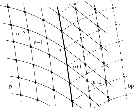
Fig. 3.10: Stencil geometry with overlapping grids. - •
Synchronize the auxiliary variables.
As we will derive the auxiliary variables for the calculation of the Laplacian in first order form (3.37), we need their correct values also on the ghost zones. These are not known, neither in patch nor in patch , but they can be calculated by interpolation from . This calculation is done in GZPatchSystem using one-dimensional interpolation in the direction parallel to the boundary. In Fig. 3.10 GZPatchSystem uses the empty circles in the nominal domain of along the two coordinate lines parallel to the thick boundary line to calculate the values of the auxiliary variables on the full circles. - •
Rotate the auxiliary variables.
For the calculation of the auxiliary variables on the ghost zone of patch , we need a transformation in accordance with the rotation of the frame. We set where the rotation matrix is calculated as in (3.35). For this calculation we have two options:- –
Analytic calculation: We calculate the rotation matrix analytically using the explicitly known frames and in local coordinates.
- –
Numeric calculation: We use the algebraic relation (3.35) numerically.
The code for the analytic calculation includes switches by patch number which determines the coordinates and by grid side which determines the rotation matrix (each of the 6 patches has 4 sides). The code for the numeric calculation on the other hand is very short. The solution of (3.35) can be written independent of local coordinates, so the second option results in a code which is more efficient than the input of the analytic rotation matrix. This method can also be generalized to the case in which the frame components are evolution variables and the rotation matrix is not known a priori. We choose the numeric calculation.
- –
- •
Build the Laplacian (3.37).
- •
Calculate the error by
The calculation in low resolution is made with 20 points, the medium one with 40 points and the high one with 80 points in both angular directions on each patch. The radial domain of calculation is .
| low-med | med-high | ||||||
| (0,5) | (1,3) | (2,4) | (0,5) | (1,3) | (2,4) | ||
| 1 | 0 | 3.96 | 3.96 | 3.96 | 3.99 | 3.99 | 3.99 |
| 1 | 1 | 3.96 | 3.96 | 3.96 | 3.99 | 3.99 | 3.99 |
| 2 | 0 | 3.94 | 3.95 | 3.95 | 3.99 | 3.99 | 3.99 |
| 2 | 1 | 3.95 | 3.95 | 3.95 | 3.99 | 3.99 | 3.99 |
| 2 | 2 | 3.95 | 3.94 | 3.94 | 3.99 | 3.99 | 3.99 |
| 3 | 0 | 3.92 | 3.94 | 3.94 | 3.98 | 3.98 | 3.98 |
| 3 | 1 | 3.93 | 3.93 | 3.94 | 3.98 | 3.98 | 3.98 |
| 3 | 2 | 3.93 | 3.93 | 3.93 | 3.98 | 3.98 | 3.98 |
| 3 | 3 | 3.94 | 3.92 | 3.93 | 3.98 | 3.98 | 3.98 |
In Table 3.1 convergence factors are listed for the second order form of the Laplacian. They are calculated in the -norm for up to on a sphere with radius . The convergence factors are independent of the sphere on which they have been calculated. For their calculation I used the code reduce by Christian Reisswig available from [137] including documentation. The factors have been given for pairs of patches that use the same coordinate system. We see a clean fourth order convergence. Note that for the calculation of the Laplacian in second order form, we do not need any synchronization.
| low-med | med-high | ||||||
| (0,5) | (1,3) | (2,4) | (0,5) | (1,3) | (2,4) | ||
| 1 | 0 | 3.33 | 3.02 | 3.02 | 3.17 | 2.96 | 2.96 |
| 1 | 1 | 3.00 | 3.33 | 3.00 | 2.96 | 3.17 | 2.96 |
| 2 | 0 | 3.75 | 4.06 | 4.06 | 3.51 | 3.61 | 3.61 |
| 2 | 1 | 2.82 | 2.84 | 2.88 | 2.90 | 2.91 | 2.92 |
| 2 | 2 | 4.09 | 3.79 | 3.79 | 3.58 | 3.46 | 3.46 |
| 3 | 0 | 3.31 | 3.21 | 3.21 | 3.18 | 3.12 | 3.12 |
| 3 | 1 | 3.23 | 3.21 | 3.42 | 3.14 | 3.11 | 3.23 |
| 3 | 2 | 3.04 | 3.30 | 3.30 | 3.02 | 3.17 | 3.17 |
| 3 | 3 | 3.27 | 3.23 | 3.20 | 3.14 | 3.13 | 3.12 |
Table 3.2 lists convergence factors for the first order form of the Laplacian. We see that the calculation is roughly third order accurate. At first sight it seems that a higher number of grid points results in a drop of convergence which would be problematic. A closer look, however, reveals that the convergence factor approaches consistently 3 when we increase the resolution as seen for example in the case with and . The study of point-wise convergence factors using gnuplot or reduce shows that the convergence on the ghost points is third order which dominates in the -norm.
The reason seems to be the interpolation of spatially derived functions and not the rotation. This claim can be tested by synchronizing the derivatives as covariant tensors instead of synchronizing the frame-based auxiliary variables as functions. In that case no rotation is needed, but the spatial derivation is interpolated and derived again for the calculation of the Laplacian. One observes a similar behavior of the convergence factors as in Table 3.2.
In an evolution scheme, a grid function that is derived on a time step is not interpolated because synchronization takes place immediately after each evolution step in the MoL_PostStep schedule bin of Cactus (see [137] for a documentation on schedule bins of Cactus). The next subsection discusses a test case with a simple evolution system where we see fourth order convergence as expected. The issue with the interpolation of numerical derivatives will not play any role in our later discussions.
3.6.4 Wave equation with source terms
As a simple test for an evolution system, we solve the wave equation on a Minkowski background for a scalar function with source
Writing out the equation in terms of frames we get
The above system can be brought into first order form by using auxiliary variables , which obey an integrability condition . Take to be a timelike frame field and to be spacelike frame fields. The evolution system reads in terms of the frame and the connection coefficients
For the tests we use the Minkowski background in standard spherical coordinates with taken to be the radial direction. The wave equation takes the form
| (3.38) |
An explicit solution to this symmetric hyperbolic system is given with the source term , by with
| (3.39) |
where is some constant. The evolution consists of the following steps:
- •
Fix the geometry.
We set the frame fields and the connection coefficients as in 3.6.3. - •
Set initial data.
The initial data consists of and calculated from the explicit solution (3.39) in Cartesian coordinates. Note that the input for the auxiliary variables depends on the frame and therefore also on the patch number. - •
Transform the data to each patch’s local coordinate system.
- •
Calculate the right hand side of the system (3.6.4) and apply boundary conditions for integration using method of lines.
No boundary conditions are needed in the angular directions. The boundary conditions we apply in the radial direction are the same as for the reduced general conformal field equations. We set the derivatives at the outer boundary to zero. - •
Do an evolution step.
- •
Analyze the numerical solution.
Our analysis consists of building the difference between the numerical solution and the analytic solution given by (3.39). - •
Synchronize the auxiliary variables .
This step is discussed in some detail below. - •
Calculate the right hand sides and apply boundary conditions.
- •
Do an evolution step …
Due to its importance in the code, we go through the steps included in the synchronization. We use the frame components to illustrate the steps involved. We write a two-dimensional frame field in angular coordinates on a patch with grid points as . The frame, the coordinates, the coordinate basis, and the grid points of a neighboring patch will be denoted by barred indices. A synchronization step transforms the information from a neighbouring patch into the current patch . The steps of the synchronization are (compare Fig. 3.10)
| Copying into current patch: | ||
| Point transformation: | ||
| Transformation of coordinate basis: | ||
| Interpolation: | ||
| Frame rotation: |
The steps except the rotation are implemented by Thornburg in GZPatchSystem.
There are three main sources of numerical errors in our evolution system that can be controlled to some degree: the round-off, the interpolation and the finite differencing. The convergence factors presented below show that round-off and interpolation errors are negligible compared to finite differencing errors. Of course, this can only be expected in a high enough resolution and a higher interpolation order than the order of finite differencing. For the tests presented below a 6th order interpolation has been chosen.
Table 3.3 shows convergence factors for the numerical solution of the symmetric hyperbolic wave equation (3.6.4). The source terms have , and . The convergence factors in Table 3.3 have been calculated on a sphere with .
| , | , | |||
|---|---|---|---|---|
| time | low-med | med-high | low-med | med-high |
| 0.0125 | 4.000 | 4.001 | ||
| 0.025 | 3.995 | 3.999 | 4.003 | 3.999 |
| 0.0375 | 3.998 | 3.998 | ||
| 0.05 | 3.994 | 3.997 | 3.999 | 3.994 |
| 0.0625 | 3.995 | 3.990 | ||
| 0.075 | 3.992 | 3.994 | 3.994 | 3.987 |
| 0.0875 | 3.992 | 3.984 | ||
| 0.1 | 3.974 | 3.990 | 3.981 | 3.981 |
We see fourth order convergence. Tests with other choices of parameters result in the same qualitative convergence behavior with slightly different numerical factors.
3.7 Implementation of the cylinder at infinity
In the previous section we discussed the principles of a frame-based evolution code using overlapping grids. In this section we will apply this technique in a local study of spatial infinity represented as a cylinder. The spacetime under study is the same as in 3.5. We use a spherical grid topology instead of a Cartesian one. The code is designed to be usable also in studies of spacetimes with non-vanishing ADM-mass.
We make some remarks on the structure of the reduced general conformal field equations with respect to the cylinder at infinity. The system consist of ordinary differential equations and the Bianchi equation for the rescaled Weyl tensor that implies a symmetric hyperbolic system as in (3.15). In coordinates , , and we can write the Bianchi equation in the form
A rescaling with , leads to the blow-up of spatial infinity to a cylinder which acts as a boundary surface to our evolution equations. This does not imply an initial boundary value problem as the boundary is totally characteristic in the sense that on [61, 62] . We get interior symmetric hyperbolic equations on and no prescription of boundary data is required or allowed. The solution is determined uniquely by Cauchy data.
The blow-up of spatial infinity takes care of the singular behavior of conformal initial data for non-vanishing ADM-mass (3.2), such that we get a regular finite initial value problem near spatial infinity. This delicate interplay between the regularization of the conformal data for the field equations and the blow-up procedure of spatial infinity is the main reason for insisting on a spherical grid topology for our numerical calculations. The procedure distinguishes radial and angular directions in a substantial way. The smoothness of conformal data and the property that is a totally characteristic surface is related to the vanishing of the radial frame vector field on the cylinder. We can implement radial and angular frame vector fields also in Cartesian coordinates, so that the radial and angular directions are distinguished geometrically near the totally characteristic surface . The points of the cylinder, however, would not correspond to points of our grid and this might require a more complicated numerical boundary treatment. The massless case studied in this section might still be numerically stable, but the code might not be applicable in studies of physically interesting spacetimes.
Another remark concerns the time evolution. As described in [62], certain entries of the matrix valued function vanish on the set where null infinity meets spatial infinity. This degeneracy of the evolution equations is the main difficulty in clarifying the open problems regarding the regular finite initial value problem near spatial infinity. It causes also numerical difficulties. Remember that we build in the calculation of the right hand side. This calculation is singular at where the matrix is degenerate. The main feature that allows us to deal with this problem is that the location of is known a priori. A suitable choice of time stepping and freezing the evolution in the unphysical domain takes care of this issue, at least in the massless case that we study. Whether this treatment of the problem is sufficient in cases with non-vanishing mass remains to be seen.
3.7.1 The initial data
For numerical calculations with GZPatchSystem we do not map spatial infinity to as we did in the Cartesian case. Instead we map spatial infinity to a finite coordinate radius. The reason is that spherical coordinates are not well-defined at the origin. Therefore GZPatchSystem assumes that the computational domain is a shell bounded by two spheres with non-vanishing radial coordinate values.
We compactify the physical Weyl solution such that the interval is mapped to via the coordinate transformation
It might better reflect the physical relations to map spatial infinity to some large radius and change the sign in the coordinate transformation so that large values of the compactifying radial coordinate correspond to the far field zone away from the source of radiation. In our case, however, we are only interested in a neighborhood of spatial infinity and not in the source. Therefore we have made the above choice of a compactifying radial coordinate.
The conformally rescaled metric in these compactifying coordinates takes the form (compare (3.26))
The Curzon solution from which we calculate conformal data is given by and . The metric is analytic at spatial infinity so it can be extended beyond . We can use the conformal factor as before to generate initial data from . Another option is to use the frame adapted to and the conformal factor . I have done the calculation presented below using the pair .
A frame adapted to reads in spherical and Cartesian coordinates as
The frame is used on the equatorial patches . On the polar patches around the -axis, we choose a different frame which is adapted the to local coordinates of the -patches in the sense of section 3.6.2. The frame is given in Cartesian coordinates by
where . This frame is by construction regular at . While the input of the frame into GZPatchSystem is made in Cartesian coordinates, the calculation of initial data using this representation is difficult because none of the components of the frame vector fields vanish and all coordinates appear many times in the expressions. Instead, for the calculation of the conformal initial data we use the frame written in spherical polar coordinates as
with . Components of the frame in this coordinate representation become singular at the poles given by and these points are part of the patches , but this is a coordinate singularity of the coordinates and not a singularity of the frame as discussed in section 3.6.2 on a simple example. We do not evaluate the above expressions on the patches . We use it for the analytic calculation of the initial data as described in 3.2.2. After the calculation has been done, we transform the data to regular Cartesian coordinates for the input. Because the frame is geometrically regular on the patches , the calculated data will also be regular. One should reorganize the result of the calculation such that no formal divisions by the coordinates and appear (with formal division I mean expressions of essentially the form ). Divisions by will appear, but they cause no problems because on the patches we have . That such a reformulation can be done is due to the regularity of the data. It is a lengthy but a useful test to calculate the conformal data using the frames and and to check that the rotation of frame-based tensors agrees with the rotation of the frames on the initial hypersurface.
Another point concerning the input of initial data into the evolution code is the divisions by appearing in the construction of initial data (3.18, 3.19). Though the data extends analytically through , a straightforward evaluation of the input causes problems. Therefore, we evaluate the formula analytically at .
The calculation of the full data set described in 3.2.2 results in long expressions that will not be given as they are not relevant for our discussion.
3.7.2 Form of and the computational domain
Looking at the initial data for the frame we observe that the components of the angular frame field become singular at which corresponds to spatial infinity . The rescaling with results in the blow-up of the point to a sphere . It leads to regular angular frame vector fields while the frame vector field in the radial direction vanishes on .
A simple choice for motivated by the regularization of conformal data would be . Fig. 3.11 shows the resulting coordinate representation of the cylinder, , and null infinity, . The value of the time coordinate on is seen to depend on the angular coordinate in a way that seems bad for numerical calculations. It decreases as we move away from the cylinder in certain directions so that future null infinity is running backwards in grid time. This behavior leads to singularities in the numerical solution once the conformal geodesics approach .

We have complete control over the form of . A good choice in the asymptotic region that we studied also in 3.1.3 seems to be
| (3.40) |
with positive real parameters and . The parameter determines the height of the cylinder at , the parameter determines the slope of (see Fig. 3.12).

3.7.3 The code
The code is based on the Cactus infrastructure [137] and uses the thorn GZPatchSystem [136]. We use second order finite differencing and fourth order Runge-Kutta time integration. No dissipation terms have been added to the evolution equations.
We solve the reduced general conformal field equations numerically on the radial computational domain . The time domain is given by . We stop the evolution after has been reached and one time step into the unphysical spacetime has been calculated. A reason for stopping the evolution is that the numerical solution in the unphysical region becomes singular near the set where spatial infinity meets null infinity. Another reason is computational efficiency. We are not interested in the domain beyond .
The fact that a large part of our field equations consist of ordinary differential equations plays a simplifying role in the implementation of the spherical grid geometry. We need to implement the rotation of frame-based variables, but only for those for which numerical derivatives need to be calculated. These are the 10 components of the rescaled Weyl tensor. We do not need to implement the rotation for the remaining 45 variables. This leads to a simplification in the synchronization step. If the evolution of the frame components and the connection coefficients is governed by partial differential equations (such as for the Friedrich-Nagy system [68]), the rotation might cause difficulties with GZPatchSystem because for the derivative of the transformation of the connection coefficients we would need to derive synchronized frame variables.
As the geometry is not given a priori, the rotation matrix is calculated after each evolution step from the evolved frame components. We proceed in this calculation as follows:
- •
After an evolution step and before the synchronization we store the components of the evolved frame field of the local patch in a temporary grid function.
- •
We synchronize, without rotation, the 10 components of the rescaled Weyl tensor, and also the frame field although no numerical derivatives of the frame field need to be calculated.
- •
After the synchronization step, the temporary grid function has the information on the local frame field while the synchronized frame field corresponds to the frame field of the neighboring patch. By using this information we calculate the rotation matrix on the ghost zone via (3.35).
- •
We rotate the components of the rescaled Weyl tensor as covariant two-tensors. After this step we can build derivatives and proceed with the evolution.
We have two disjoint numerical boundaries in contrast to the evolution with point compactification at spatial infinity. The inner boundary in the physical domain (the outer boundary of the computational domain) is as in the Cartesian case an artificial timelike surface. Our treatment consists of freezing the evolution at this artificial boundary which is not a well-posed treatment. We emphasize again that in the physically interesting cases no artificial boundary will be present. As this inner boundary is not a general feature of the method we develop, we are not concerned with this issue.
The boundary which was not present in the Cartesian case is given by the cylinder at infinity. The cylinder is the natural boundary to our evolution system. It is a characteristic surface so that no boundary data are to be prescribed. Further, as it is totally characteristic, no radial derivatives need to be calculated. Therefore no one-sided differencing needs to be implemented on the cylinder. For second order accurate finite differencing (3.29) also the next point to the cylinder does not require any special treatment.
3.7.4 The radiation field
The form of in our choice of does not depend on angular coordinates as seen in Fig. 3.12. Therefore, on , the angular derivatives of the conformal factor vanish.

Fig. 3.13 shows calculated along in the direction of the Cartesian -axis. We observe the same qualitative behavior as in Fig. 3.9. The radiation field grows as we move to the interior of the spacetime. The numerical values depend on the choice of the free function . The parameter that determines the height of the cylinder at according to (3.40) is chosen to be small so that we can calculate a piece of before the ill-posed inner boundary treatment can destroy the solution. For the evolution leading to Fig. 3.13 we have chosen and .
No quantitative comparison has been made between the calculation with the one-point compactification and with the cylinder. Certainly, more tests and experiments can be done in the massless axisymmetric case. It seems, however, more interesting to move on to studies of spacetimes with non-vanishing ADM-mass using further developed numerical methods. This will be part of future work.
3.8 Discussion
The main content of this chapter has been the development of a numerical method that allows us to construct solutions to the Einstein equations including spatial and null infinity by solving a regular finite initial value problem near spatial infinity based on the reduced general conformal field equations. We have implemented this system numerically with spatial infinity represented as a cylinder.
The method presented in this chapter is based on solving a frame-based evolution system with smooth inner and outer boundaries. Certain difficulties we had to deal with are specific to numerical calculations, such as the coordinate and the frame singularity on spheres. Other difficulties, such as the degeneracy of the equations at the set where spatial infinity meets null infinity are shared by the numerical and analytic studies. It would be interesting to see whether our numerical treatment can deal with some mild singularity of the conformal structure at null infinity.
We have studied a neighborhood of spatial infinity of a radiative massless spacetime. The study of spacetimes with non-vanishing ADM-mass may require technical improvements of the code. We may use higher order information on the solution along the cylinder from analytic studies [61, 141]. Parallelization would allow more extensive and accurate studies of the spacetimes in question. A possibility would be to use parallel multi-block methods to solve evolution systems using multiple patches [92, 125].
As shown in conformal diagrams of section 3.1, the speed of outgoing characteristics approaches zero near spatial infinity. This property may be used to construct adapted finite differencing stencils. One should also consider adapting the stencil to the a priori known location of such that boundary grid points lie on . For long time evolutions aiming at timelike infinity, one may add additional grid points dynamically into the computational domain such that the resolution loss due to the form of is compensated numerically.
A major advantage of the conformal Gauss gauge is that the location of the conformal boundary can be prescribed a priori in terms of coordinates and initial data by the choice of a free function , assuming the underlying conformal geodesics are well-behaved. A convenient choice for numerical calculations seems to be (3.40). Given a time scale and an accuracy requirement, we may choose a very large that would allow an efficient and accurate calculation of gravitational radiation in the conformal Gauss gauge without much resolution loss in the physical part of the conformal extension. It is an open issue which choices of are good in the interior of asymptotically flat spacetimes. We have seen in numerical solutions of conformal geodesics on given backgrounds, that certain choices of are bad in the interior of black holes. These problems seem, however, of secondary importance. The main question that one should study concerns the feasibility of the conformal Gauss gauge in general studies of the asymptotic region. If it turns out that the conformal geodesics are not well-behaved in the interior region, one can still devise matching methods or choose another gauge in a domain where the conformal factor has been set initially to unity. One can only hope to answer the question on the feasibility of the conformal Gauss gauge gradually. Possible steps for further research are outlined in section 4.2.
Chapter 4 Summary and Outlook
In this thesis I took a conformal approach to the numerical calculation of asymptotically flat spacetimes. To avoid certain conceptual and technical deficiencies of current numerical methods discussed in the introduction, I devised and studied new numerical methods which have, as expected, difficulties of their own.
In the summary I discuss the achievements of the thesis and point out some open problems of the methods introduced. In the outlook I try to give a glimpse of the possibilities opened up by the methods assuming their problems can be solved. The thesis ends with remarks on the idea of conformal infinity.
4.1 Summary
The question that has been raised in the preface concerns the numerical methods for calculating asymptotically flat spacetimes, not the statements that can be made on such spacetimes. Accordingly the main content of this thesis does not lie in numerical studies of the solution space to the Einstein equations but in the development of new methods for future studies of the solution space. I tried to motivate the search for new methods in the introduction by stating some problems of currently available numerical methods. The results of this thesis have been presented in two chapters, each concentrating on a different asymptotic domain: null infinity and spatial infinity.
Chapter 2. Null Infinity
- •
Construction of a -fixing gauge in spherical symmetry, 2.2.
This study refutes claims made at various places (for example in [29]) that the conformal approach necessarily leads to a resolution loss in the physical spacetime. The explicit examples written in a -fixing gauge in spherical symmetry show clearly that the allegedly necessary resolution loss is a property of a bad coordinate choice and not of the conformal approach itself, a fact sufficiently supported by existence results. The examples also serve as a testbed for new ideas in the conformal approach.
- •
The development of a numerical method that includes null infinity in the computational domain to solve a hyperboloidal initial value problem for the Einstein equations in a general wave gauge, 2.3, 2.4.
A basic difficulty with the equations used in the conformal approach has been that they are very different from common formulations of the Einstein equations. Experience gained within the standard approach could so far not be applied in the conformal approach, and the clean framework that the idea of conformal infinity yields could not be used in conventional numerical relativistic calculations. Motivated by this difficulty, I constructed a method to include null infinity in the computational domain using a common reduction of the Einstein equations.
Assuming hyperboloidal initial data whose maximal development admit a smooth conformal boundary, I showed that a -fixing gauge can be constructed during the solution of a hyperboloidal initial value problem using a suitable coupling of the conformal and the coordinate gauge freedom in a general wave gauge. This result opens up the possibility to attach smoothly a conformally compactified asymptotic region, where conformal techniques are applied, to successful numerical calculations of the interior domain in a direct way, using the same set of variables and the same set of equations.
- •
A numerical test of the introduced method in spherical symmetry, 2.5.
The main difficulty with the aforementioned method is the appearance of formally singular terms in the evolution equations. Within the class of spacetimes that admit a smooth conformal boundary and in a -fixing gauge, each of these terms attains at null infinity a regular limit. This limit can, in principle, be calculated by numerical methods. One can not assert without extensive numerical studies, however, that such a calculation will, in practice, result in a numerically stable code for highly dynamical spacetimes. As a first test I studied the spherically symmetric case in a stationary gauge using simple numerical methods. One could observe, in this special case, that a numerical treatment of the outer boundary based on extrapolation of the variables allows the calculation of a piece of null infinity.
Chapter 3. Spatial Infinity
The hyperboloidal approach does not allow us access to spacetimes in their entirety. To make statements on global properties of spacetimes one would like to get access to the conformal boundary including spatial infinity. The main problem in this context is the singular behaviour of conformal initial data at spatial infinity for non-vanishing ADM-mass. This problem was treated by Friedrich who formulated a regular finite initial value problem near spatial infinity using the reduced general conformal field equations. The construction allows a smooth extension of conformal data with non-vanishing ADM-mass through spatial infinity which is blown up to a sphere on the initial hypersurface. The development of the data results in a representation of spatial infinity as a cylinder. Currently the only system that allows a numerical study of spatial infinity including a piece of null infinity is given by the reduced general conformal field equations. The following steps have been taken in the course of a numerical implementation of this system.
- •
Numerical construction of a conformal Gauss gauge on the Schwarzschild-Kruskal and the Kerr spacetimes, 3.1.
The reduced general conformal field equations are based on the conformal Gauss gauge. Though it has been shown analytically that the conformal Gauss gauge is well-behaved in strong field regions in spherical symmetry [63], the general behavior of the underlying conformal geodesics is unknown. Besides, it can not be guaranteed that analytical methods work well in numerical calculations. To test the numerical feasibility of the conformal Gauss gauge I reproduced the analytic construction of a conformal Gauss gauge in the Schwarzschild-Kruskal spacetime covering the entire spacetime in a smooth way. Going beyond available analytical studies I found out numerically that one can also cover the Kerr spacetime using conformal geodesics including null infinity, timelike infinity and the Cauchy horizon.
- •
Numerical simulation of an entire, asymptotically flat, black hole spacetime, 3.3.
As a first test of the numerical feasibility of the reduced general conformal field equations, I solved a Cauchy problem based on this system in spherical symmetry with data from the Schwarzschild-Kruskal spacetime. The equations in spherical symmetry become a system of ordinary differential equations. This is a major simplification so that no statements on the applicability of the system in the general case can be deduced from this study. It should still be noted that this is the first numerical calculation of an entire, asymptotically flat black hole spacetime including spacelike, null and timelike infinity and the region close to the singularity.
- •
Numerical calculation of a radiative spacetime including spatial infinity and a piece of null infinity, 3.5.
In order to study cases with non-vanishing gravitational radiation, I wrote an evolution code for the reduced general conformal field equations based on a three dimensional Cartesian grid using the software infrastructures Cactus [137] and Kranc [83]. This code can only deal with the one point compactification at spatial infinity which results in singular conformal data for non-vanishing ADM-mass. Therefore I calculated asymptotically flat, axisymmetric initial data based on studies by Friedrich which have vanishing ADM-mass but whose development has a non-vanishing radiation field. I analyzed the numerical development of this data and showed that the radiation content of the spacetime does not vanish but grows towards the interior where presumably a naked singularity resides.
- •
The development of a three dimensional code to solve Cauchy problems for frame-based evolution systems with smooth inner and outer boundaries, 3.6.
I wrote a numerical code within the Cactus infrastructure [137] using a Cactus thorn written by Thornburg [136] which implements spherical coordinates using multiple patches. I extended this infrastructure to include frame rotations so that Cauchy problems for frame-based evolution systems can be solved numerically.
- •
Numerical studies of spatial infinity represented as a cylinder, 3.7.
In the representation of spatial infinity as a cylinder, the equations degenerate at the set where the cylinder meets null infinity. This difficulty has been dealt with by freezing the evolution in the unphysical domain and choosing a time stepping that avoided an evaluation of the equations at the critical set. An essential property of the conformal Gauss gauge which allows us such a treatment of the problem is the a priori knowledge of the conformal factor in terms of initial data and grid coordinates. I suggested a convenient choice for the remaining gauge freedom in the conformal Gauss gauge for numerical calculations. I did numerical studies of the cylinder in the massless, axisymmetric case which is special in the sense that the spacetime under study allows the one-point compactification.
The main open problem with this approach is related to the degeneracy of the equations at the critical set. Extensive studies and sophisticated numerical techniques are required before this approach can be applied to study interesting mathematical and physical questions concerning the asymptotic behavior of solutions to Einstein equations.
The studies show that the a priori knowledge of the conformal factor is a very convenient feature in numerical studies. It seems essential that the conformal boundary and also the conformal factor should be controlled to some degree in a numerical calculation. One can expect that this feature will play an important role in the future development of the conformal approach.
4.2 Outlook
The discussed methods suggest a wide range of prospects to study the solution space to the Einstein equations in a way that has not been possible before. Some suggestions are listed below.
- •
A simple but illustrative experiment would be to solve a wave equation on the Schwarzschild and the Kerr spacetimes written in a -fixing gauge using a three dimensional code that can handle spherical grid topology. This might allow an accurate study of quasi-normal modes and tail behaviour.
- •
The method of solving an hyperboloidal initial value problem for the conformally transformed Einstein equations in a general wave gauge by prescribing the coordinate representation of a conformal factor should be tested in three dimensions for dynamical spacetimes. The basic infrastructure required for this test is already available [106] so that one can concentrate on the main intrinsic problem of the method, namely the numerical calculation of the formally singular terms in the course of the evolution.
- •
- •
One should construct hyperboloidal initial data for a radiative spacetime admitting a smooth conformal boundary. There are many interesting and open questions related to the interpretation of hyperboloidal data that may be studied by evolving them.
- •
A straightforward test of the numerical techniques presented in chapter 3 would be to evolve conformal data corresponding to static or stationary spacetimes with non-vanishing ADM-mass in a neighbourhood of spatial infinity and to check that their radiation field vanishes.
- •
One should construct solutions with a complete initial hypersurface so that no artificial inner boundary needs to be introduced. The question how to construct numerically initial data for spacetimes which admit a smooth conformal boundary is open. Data whose development leads to some mildly singular behavior at null infinity can be constructed by solving numerically a Lichnerowicz equation for the initial conformal factor [43]. To numerically calculate conformal initial data for the reduced general conformal field equations one needs to build numerical divisions of the data by the conformal factor 3.2.2. This might not to be an easy task, but it seems worth the effort. A numerical study on smoothness properties of solutions near null infinity has not yet been done. A strong interaction between mathematical and numerical studies in this question might give new impulses in both directions.
- •
Another interesting study related to the asymptotic behavior of solutions to the Einstein equations would be to evolve data which might results in different degrees of smoothness at future and past null infinity as suggested in [142].
- •
- •
One might try to use use the conformal Gauss gauge in a metric formulation Einstein equations. This might lead to a simplification in the equations and require less variables.
- •
The implementation of a frame-based evolution system should allow us to implement the Friedrich-Nagy system [68]. An interesting study with a successful implementation of the Friedrich-Nagy system and the reduced general conformal field equations would be to evolve a simple but radiative spacetime both with and without an artificial, timelike outer boundary. This would allow us to compare the approximation given by the timelike outer boundary at a finite distance away from the source with the idealization given by conformal infinity such that systematic errors can be estimated for different kinds of boundary data. Studies along these lines have been made without numerical access to null infinity using solutions for which accurate analytic expectations can be calculated [106, 118].
One of the motivations behind the work of this thesis has been to develop techniques to calculate numerically entire, asymptotically flat, radiative spacetimes. This still remains an important goal for future work. A combination of numerical calculations near spatial infinity and null infinity might allow us to accomplish this task. An achievement of this goal would deliver a starting point for extensive studies of the solution space to the Einstein equations using numerical methods based on rigorous analysis.
4.3 Concluding remarks
A general critique concerning the concept of null infinity and its role in physical questions holds that null infinity is ”too far away”. After all, the Earth where we are doing our measurements is not infinitely far away from the sources and we do not move along null geodesics in contrast to an observer along null infinity.
In the Schwarzschild spacetime, we have a length scale at our disposal, so we can discuss astrophysical distances in numerical calculations. To give a notion for the scales in the conformal diagram Fig. 3.2, three curves with constant Schwarzschild radius have been plotted. The curve at Schwarzschild radius corresponds to about km for a black hole with four solar masses but it can hardly be distinguished from in the conformal diagram. Even if we consider super-massive black holes, the distance corresponding to is incomparably small contrasted to the thousands or millions of light years that separates us from the astrophysical sources. In this representation, the numerical effort for simulating the region from to is very small whereas in the standard approach putting the outer boundary from to costs considerable effort in terms of numerical techniques and computational sources. We note that this behavior depends on the conformal gauge. One has the freedom to set initially on a given domain if more resolution is desired in that domain. Further, we have seen in chapter 2 that a positive smooth function for the coordinate representation of the conformal factor may be prescribed in the context of the hyperboloidal initial value problem such that certain spacetime domains can be emphasized for the calculation while still compactifying the asymptotic region. We may conclude that the conformal compactification technique is not only promising for an unambiguous outer boundary treatment and radiation extraction, but also for a computationally efficient numerical code to deal with the asymptotic region.
If some astrophysically motivated length scale can be determined, as suggested for example in [37], such that an observer ”nearly at rest in the frame of the isotropic cosmic microwave background radiation” at that distance from the source can regard the source as isolated, this length scale will naturally be given in astronomical units. The example above shows that a timelike curve at such a distance away from the source is almost indistinguishable from in the conformally compactified picture while the standard approach does not even allow the discussion of such length scales. Therefore, the arguments presented in [37] can as well be considered as supporting the notion of conformal infinity. After having calculated the entire spacetime, we can still discuss the calculation of a field which represents radiation (having a proper limit with respect to an adapted tetrad at null infinity to which we would have direct access) on a timelike surface arbitrarily far away from the source of radiation. Within the standard approach, however, it seems hardly possible to calculate an astronomical domain for an isolated system.
In this context, I would like to emphasize that the idea of conformal infinity is an idealization, in contrast to an approximation. The difference can be illustrated on the idea of a number, say a real number. We do not have physical access to real numbers. Results of measurements are in a sense fuzzy. They are given in terms of rational numbers with error bars regarded as approximations to real numbers. Physics without real numbers would be, however, very inconvenient. Most physicists would agree that the notion of a real number is a useful one. The idealization of a real number allows a clean modeling in various fields of science. Similarly, the concept of conformal infinity allows a clean modeling in general relativity.
In [37] it is stated that the conformal approach implies ”introducing an arbitrary amount of empty space not reflecting astronomical reality”. A similar statement can be made concerning real numbers by claiming that they imply an arbitrary amount of accuracy beyond the Planck scale not reflecting physical reality. The question whether real numbers are real in an ontological sense belongs, however, to the realm of philosophy. If an idealization allows a clean modeling of the ’actual reality’ we can observe and if it is of practical use, than it is a viable physical viewpoint to use the concept while being aware of the limits of its application.
Another argument claims that there is not much motivation for using the idea of conformal infinity, especially regarding the impressive milestones achieved recently within the standard approach. While a case can be made that the deficiencies of the standard approach are not relevant for the detection of gravitational waves as the accuracy of the waveforms seems to be enough for detection, there is also the viewpoint holding that interesting physics will be hidden behind the first couple of digits in the observational data. Having predictions which are accurate only up to a couple of percents due to systematic errors will most probably not be enough to answer many interesting questions in the prospective field of gravitational wave astronomy. One should also not forget that beside the effort of calculating waveforms there remains the task of exploring the solution space. Here it is unclear how useful the conventional approaches are if global questions are concerned.
If an objection is to be made against the conformal approach, I believe, it should be made not on conceptual but rather on practical grounds. Whatever level of conceptual clarity, geometric appeal or computational efficiency the conformal approach promises, in the end, its application in numerical relativity must be judged after its practicability in numerical studies of the solution space to the Einstein equations.
It seems to me that the most important task for future work in the context of our discussion is to devise from the conformal approach a practical tool for numerical calculations of asymptotically flat spacetimes. This could not be achieved yet for the calculation of highly dynamical, asymptotically flat spacetimes. Unfortunately, the results presented in this thesis also do not allow the conclusion that the suggested methods can be used in general calculations. I believe that this task can only be managed if insights that have been gained in the standard approach can be conveniently combined with the calculation of the asymptotic region. The ideas presented in this thesis, especially the a priori knowledge of the conformal factor in numerical calculations, seem promising to accomplish this task. One may hope that future work will allow us to construct from the beautiful idea of conformal infinity a practical tool for numerical calculations.
Appendix A Calculation of causal diagrams
In this appendix, we present how Penrose diagrams like Fig. 1.2 or Fig. 2.7 and radial light rays on the grid like in Fig. 1.5 or in Fig. 2.5 for a given Schwarzschild-Kruskal background are calculated. We omit angular dimensions.
A.1 Penrose diagrams
The two-dimensional Schwarzschild metric in standard coordinates is given by
The coordinate singularity at the event horizon can be removed by introducing advanced and retarded null coordinates
| (A.1) |
The Schwarzschild metric in these coordinates takes the forms
| (A.2) |
These line elements can be analytically extended beyond the event horizon to .
We introduce the Kruskal-Szekeres coordinates for by and . The metric written in double-null coordinates becomes
where respectively. The Kruskal-Szekeres coordinates can be analytically extended to und . The Schwarzschild coordinates are given by the implicit relations
Compactifying coordinates can be introduced by and . These are defined in the range . We define new time and space coordinates by setting
| (A.3) |
In the Penrose diagrams, the -axis runs vertically and the -axis runs horizontally. Summarizing the coordinate relations, we have , and
| (A.4) |
The compactifying coordinates have been used to plot the Penrose diagrams of the Schwarzschild-Kruskal spacetime in Fig. 1.2 or the extended Schwarzschild spacetime in Fig. 1.5.
A.1.1 Ingoing Eddington-Finkelstein coordinates
We introduce the coordinate . The metric becomes
| (A.5) |
These coordinates are sometimes referred to as ingoing Eddington-Finkelstein coordinates in the numerical literature. The spatial surfaces that are used in a simulation based on ingoing Eddington-Finkelstein coordinates are given by the level sets of the function
To plot the surfaces in the Penrose diagram of the extended Schwarzschild spacetime in Fig. 1.5, we use (A.4) and write (see also [98])
The Schwarzschild coordinate is regarded as a parameter along the curves with constant values of . We transform the above expressions using the compactifying time and space coordinates from (A.3). The resulting curves are plotted on the -plane with Mathematica using the function ParametricPlot.
A.1.2 Constant mean curvature foliation
In Fig. 1.11 and Fig. 2.7 we plotted constant mean curvature surfaces in the extended Schwarzschild spacetime using compactifying coordinates. The properties of these surfaces have been discussed in [96].
Surfaces in the Schwarzschild spacetime that are dragged along the timelike Killing vector field can be written as level sets of a function . Here, is referred to as the height function. To find a CMC-slicing of the Schwarzschild spacetime one requires that the mean extrinsic curvature of the surfaces is constant. We get
For this can be integrated once with an integration constant . A following algebraic manipulation results in the differential equation
| (A.6) |
where is as defined in 2.2.2. We can not integrate this equation explicitly to get in closed form but we can integrate it numerically. A difficulty is the numerical integration for the function at the horizon for . The integral can be calculated in the Cauchy principal value sense [96]. We build the integral in the regions and respectively via
where is a positive small constant. We subsequently match the resulting curves together at the event horizon. The embedding of the foliation is calculated as follows. We define the embedded surfaces by level sets of a function which can be written as
so that . We use the relations (A.4) and write
The numerical integration gives us a list of pairs of . The surfaces corresponding to different values of can be plotted with Mathematica using the function ListPlot.
A.2 Null rays on the grid
To visualize the causal structure on a numerical grid for a spherically symmetric spacetime in a stationary gauge we calculate the ingoing and outgoing radial null rays with respect to grid coordinates . The metric can be written as
A parametrized null curve fulfills the relation
For , we can calculate the curve by integrating
| (A.7) |
The positive sign corresponds to ingoing null rays. In the following we discuss the visualisation of the causal structure on the grid for the Schwarzschild spacetime based on different coordinates.
A.2.1 Ingoing Eddington-Finkelstein coordinates
For Fig. 1.5 we use the form of the metric in ingoing Eddington-Finkelstein coordinates (A.5) and integrate (A.7) to get
for ingoing and outgoing null rays. We plot different light rays by varying the constants and To include the excision region in Fig. 1.5 we plot the null rays inside and outside the event horizon separately and match them together.
A.2.2 Coordinate compactification at spatial infinity
To generate the plots in Fig. 1.7 and Fig. 1.7 we introduce a compactifying radial coordinate in (A.5) by
The domain corresponds to and the event horizon is at . The metric (A.5) becomes
This metric is singular at as expected. Integration of (A.7) results in long expressions that can be written in explicit form. Note that the ingoing null rays in Fig. 1.7 that seem to come in from spatial infinity start at a small vicinity of spatial infinity.
A.2.3 Cauchy-Characteristic Matching
The left part of Fig. 1.9 has been plotted using the timelike ingoing Eddington-Finkelstein coordinates as described above. For the right part we write the Schwarzschild metric in the advanced null coordinate as in (A.2) and subsequently introduce a compactifying radial coordinate via to get
The light cones in the parametrization are then given by solutions to the differential equation
The solutions are given by
Note that we need these light rays only outside the event horizon in the matching region.
A.2.4 Constant mean curvature slicing
Bibliography
- [1] Ronald Adler, Maurice Bazin, and Menahem Schiffer. Introduction to general relativity. McGraw-Hill, New York, 1975.
- [2] Lars Andersson. Construction of hyperboloidal initial data. Lect. Notes Phys., 604:183–194, 2002. gr-qc/0205083.
- [3] Lars Andersson, Piotr T. Chruściel, and Helmut Friedrich. On the regularity of solutions to the yamabe equation and the existence of smooth hyperboloidal initial data for Einstein’s field equations. Commun. Math. Phys., 149:587–612, 1992.
- [4] Abhay Ashtekar. Asymptotic structure of the graviational field at spatial infinity. In A. Held, editor, General Relativity and Gravitation: One hundred years after the birth of Albert Einstein, volume 2, pages 1–36. Plenum Press N. Y., 1980.
- [5] Abhay Ashtekar and J D Romano. Spatial infinity as a boundary of spacetime. Class. Quant. Grav., 9:1069–1100, 1992.
- [6] Maria C. Babiuc and J.Winicour. Constraint-preserving Sommerfeld conditions for the harmonic Einstein equations. 2006. gr-qc/0612051.
- [7] Maria C. Babiuc, Béla Szilágyi, and J.Winicour. Harmonic initial-boundary evolution in general relativity. Phys. Rev. D, 73:064017, 2006. gr-qc/0601039.
- [8] Maria C. Babiuc, Béla Szilágyi, and Jeffrey Winicour. Testing numerical relativity with the shifted gauge wave. Class. Quant. Grav., 23:S319–S342, 2006. gr-qc/0511154.
- [9] John G. Baker, Joan Centrella, Dae-Il Choi, Michael Koppitz, and James van Meter. Binary black hole merger dynamics and waveforms. Phys. Rev. D, 73:104002, 2006. gr-qc/0602026.
- [10] John G. Baker, Joan Centrella, Dae-Il Choi, Michael Koppitz, and James van Meter. Gravitational wave extraction from an inspiraling configuration of merging black holes. Phys. Rev. Lett., 96:111102, 2006. gr-qc/0511103.
- [11] Robert A. Bartnik and Andrew H. Norton. Einstein equations in the null quasi-spherical gauge. III: Numerical algorithms. 1999. gr-qc/9904045.
- [12] Robert Beig and Niall O’Murchadha. Trapped surfaces due to concentration of gravitational radiation. Phys. Rev. Lett., 66:2421–2424, 1991.
- [13] Robert Beig and Niall O’Murchadha. Trapped surfaces in vacuum space-times. Class. Quant. Grav., 11:419–430, 1994.
- [14] Robert Beig and Bernd Schmidt. Einstein’s equations near spatial infinity. Commun. Math. Phys., 87:65–80, 1982.
- [15] Robert Beig and Walter Simon. Proof of a multipole conjecture due to Geroch. Commun. Math. Phys., 78:75–82, 1980.
- [16] Emanuele Berti, Vitor Cardoso, Jose A. Gonzalez, Ulrich Sperhake, Mark Hannam, Sascha Husa, and Bernd Brügmann. Inspiral, merger and ringdown of unequal mass black hole binaries: a multipolar analysis. 2007. gr-qc/0703053.
- [17] Florian Beyer. Asymptotics and singularities in cosmological models with positive cosmological constant. PhD thesis, University of Potsdam, 2007. 0710.4297.
- [18] Jiri Bicak. Selected solutions of Einstein’s field equations: Their role in general relativity and astrophysics. Lect. Notes Phys., 540:1–126, 2000. gr-qc/0004016.
- [19] Nigel T. Bishop. Numerical relativity: Combining the Cauchy and characteristic initial value problem. Class. Quant. Grav., 10:333–341, 1993.
- [20] Nigel T. Bishop, Roberto Gómez, Paulo R. Holvorcem, Richard A. Matzner, Philippos Papadopoulos, and Jeffrey Winicour. Cauchy-characteristic matching: A new approach to radiation boundary conditions. Phys. Rev. Lett., 76(23):4303–4306, 3 June 1996.
- [21] H. Bondi, M. G. J. van der Burg, and A. W. K. Metzner. Gravitational waves in general relativity VII. Waves from axi-symmetric isolated systems. Proc. R. Soc. London, A269:21–52, 1962.
- [22] John P. Boyd. Chebyshev and Fourier Spectral Methods (Second Edition, Revised). Dover Publications, New York, 2001.
- [23] Bernd Brügmann, José A. González, Mark Hannam, Sascha Husa, Ulrich Sperhake, and Wolfgang Tichy. Calibration of moving puncture simulations. 2006. gr-qc/0610128.
- [24] Yvonne Bruhat. Theoreme d’existence pour certains systemes d’equations aux derivees partielles non lineaires. Acta Mathematica, 88:141–225, 1952.
- [25] Luisa T. Buchman and J. M. Bardeen. Schwarzschild tests of the WEBB tetrad formulation for numerical relativity. Phys. Rev. D, 72:124014, 2005. gr-qc/0508111.
- [26] Luisa T. Buchman and Olivier C. A. Sarbach. Towards absorbing outer boundaries in general relativity. Class. Quant. Grav., 23:6709–6744, 2006. arXiv:gr-qc/0608051.
- [27] Luisa T. Buchman and Olivier C. A. Sarbach. Improved outer boundary conditions for einstein’s field equations. Class. Quant. Grav., 24:S307–S326, 2007. gr-qc/0703129.
- [28] Gioel Calabrese and Carsten Gundlach. Discrete boundary treatment for the shifted wave equation. Class. Quant. Grav., 23:S343–S368, 2006. gr-qc/0509119.
- [29] Gioel Calabrese, Carsten Gundlach, and David Hilditch. Asymptotically null slices in numerical relativity: Mathematical analysis and spherical wave equation tests. Class. Quant. Grav., 23:4829–4846, 2006. gr-qc/0512149.
- [30] Manuela Campanelli, Carlos O. Lousto, Pedro Marronetti, and Yosef Zlochower. Accurate evolutions of orbiting black-hole binaries without excision. Phys. Rev. Lett., 96:111101, 2006. gr-qc/0511048.
- [31] Carlo Cattani and Michelangelo De Maria. Conservation laws and gravitational waves in general relativity (1915-1918). In J. Earman, M. Janssen, and J.D. Norton, editors, The Attraction of Gravitation, pages 63–87, Basel, 1993. Birkhäuser.
- [32] S. Chandrasekhar. The Mathematical Theory of Black Holes. Oxford University Press, Oxford, England, 1983.
- [33] Matthew W. Choptuik, Luis. Lehner, Ignacio. Olabarrieta, Roman. Petryk, Frans. Pretorius, and Hugo Villegas. Towards the final state of an unstable black string. Phys. Rev. D, 68:044001, 2003. gr-qc/0304085.
- [34] Piotr T. Chruściel and Erwann Delay. Existence of non-trivial, vacuum, asymptotically simple spacetimes. Class. Quant. Grav., 19:L71–L79, 2002.
- [35] Piotr T. Chruściel, M.A.H. MacCallum, and D.B. Singleton. Gravitational waves in general relativity XIV. Bondi expansions and the polyhomogeneity of scri. Phil. Trans. Roy. Soc. Lond. A, 350:113, 1995.
- [36] J. Corvino and R. Schoen. On the asymptotics for the vacuum Einstein constraint equations. 2003. gr-qc/0301071.
- [37] D. P. G. Cox. How far is ’infinity’. Gen. Rel. Grav., 39:87–104, 2007.
- [38] Jeremy W. Crampton. Cartography’s defining moment: The Peters Projection Controversy, 1974-1990. Cartographica, 31:16–32, 1994.
- [39] H.E.J. Curzon. Cylindrical solutions of Einstein’s gravitation equations. Proc. Lond. Math. Soc., 23:477, 1924.
- [40] Mihalis Dafermos and Igor Rodnianski. A note on boundary value problems for black hole evolutions. 2004. gr-qc/0403034.
- [41] Mihalis Dafermos and Igor Rodnianski. A proof of Price’s law for the collapse of a self-gravitating scalar field. Invent. Math., 162:381–457, 2005. gr-qc/0309115.
- [42] Sergio Dain. Initial data for stationary space-times near space-like infinity. Class. Quant. Grav., 18:4329–4338, 2001. gr-qc/0107018.
- [43] Sergio Dain and Helmut Friedrich. Asymptotically flat initial data with prescribed regularity at infinity. Commun. Math. Phys., 222:569–609, 2001. gr-qc/0102047.
- [44] Peter Diener, Ernst Nils Dorband, Erik Schnetter, and Manuel Tiglio. New, efficient, and accurate high order derivative and dissipation operators satisfying summation by parts, and applications in three-dimensional multi-block evolutions. 2005. gr-qc/0512001.
- [45] Arthur Stanley Eddington. The propagation of gravitational waves. Proc. R. Soc. London A, 102:268–282, 1922.
- [46] Albert Einstein. Näherungsweise Integration der Feldgleichungen der Gravitation. Preuss. Akad. Wiss. Berlin, Sitzungsber., pages 688–696, 1916.
- [47] Albert Einstein. Über Gravitationswellen. Preuss. Akad. Wiss. Berlin, Sitzungsber., pages 154–167, 1918.
- [48] Bengt Fornberg. A Practical Guide to Pseudospectral Methods. Cambridge University Press, Cambridge, UK, 1998.
- [49] Jörg Frauendiener. Numerical treatment of the hyperboloidal initial value problem for the vacuum Einstein equations. II. The evolution equations. Phys. Rev. D, 58:064003, 1998. gr-qc/9712052.
- [50] Jörg Frauendiener. Numerical treatment of the hyperboloidal initial value problem for the vacuum Einstein equations. III. On the determination of radiation. Class. Quant. Grav., 17:373–387, 2000. gr-qc/9808072.
- [51] Jörg Frauendiener. Conformal infinity. Living Rev. Relativity, 7(1), 2004.
- [52] Jorg Frauendiener and Tilman Vogel. Algebraic stability analysis of constraint propagation. Class. Quant. Grav., 22:1769–1793, 2005. gr-qc/0410100.
- [53] Helmut Friedrich. On the regular and asymptotic characteristic initial value problem for Einstein’s vacuum field equations. Proc. Roy. Soc. London, A 375:169–184, 1981.
- [54] Helmut Friedrich. Cauchy problems for the conformal vacuum field equations in general relativity. Comm. Math. Phys., 91:445–472, 1983.
- [55] Helmut Friedrich. On the hyperbolicity of Einstein’s and other gauge field equations. Comm. Math. Phys., 100:525–543, 1985.
- [56] Helmut Friedrich. On the existence of n-geodesically complete or future complete solutions of Einstein’s field equations with smooth asymptotic structure. Comm. Math. Phys., 107:587–609, 1986.
- [57] Helmut Friedrich. On static and radiative space-times. Commun. Math. Phys., 119:51–73, 1988.
- [58] Helmut Friedrich. Einstein equations and conformal structure: existence of anti-de Sitter-type space-times. J. Geom. Phys., 17:125–184, 1995.
- [59] Helmut Friedrich. Hyperbolic reductions for Einstein’s equations. Class. Quant. Grav., 13:1451–1469, 1996.
- [60] Helmut Friedrich. Einstein’s equations and geometric asymptotics. 1998. gr-qc/9804009.
- [61] Helmut Friedrich. Gravitational fields near space-like and null infinity. J. Geom. Phys., pages 83–163, 1998.
- [62] Helmut Friedrich. Conformal Einstein evolution. Lect. Notes Phys., 604:1–50, 2002. gr-qc/0209018.
- [63] Helmut Friedrich. Conformal geodesics on vacuum space-times. Commun. Math. Phys., 235:513–543, 2003.
- [64] Helmut Friedrich. Smoothness at null infinity and the structure of initial data. In Piotr T. Chruściel and Helmut Friedrich, editors, The Einstein equations and the large scale behaviour of gravitational fields, pages 121–203, Basel, 2004. Birkhäuser.
- [65] Helmut Friedrich. Is general relativity ‘essentially understood’ ? Annalen Phys., 15:84–108, 2005. gr-qc/0508016.
- [66] Helmut Friedrich. On the non-linearity of the subsidiary systems. Class. Quant. Grav., 22, 2005. gr-qc/0504129.
- [67] Helmut Friedrich. Static vacuum solutions from convergent null data expansions at space-like infinity. 2006. gr-qc/0606133.
- [68] Helmut Friedrich and Gabriel Nagy. The initial boundary value problem for Einstein’s vacuum field equations. Commun. Math. Phys., 201:619–655, 1999.
- [69] Helmut Friedrich and Alan D. Rendall. The Cauchy problem for the Einstein equations. Lect. Notes Phys., 540:127–224, 2000. gr-qc/0002074.
- [70] Helmut Friedrich and Bernd Schmidt. Conformal geodesic in general relativity. Proc. Roy. Soc. London, A 414:171–195, 1987.
- [71] Helmut Friedrich and John Stewart. Characteristic initial data and wavefront singularities in general relativity. Proc. R. Soc., A385:345–371, 1983.
- [72] David Garfinkle. Harmonic coordinate method for simulating generic singularities. Phys. Rev. D, 65:044029, 2002.
- [73] Adrian P Gentle, Daniel E. Holz, Arkady Kheyfets, Pablo Laguna, Warner A. Miller, and Deirdre M. Shoemaker. Constant crunch coordinates for black hole simulations. Phys. Rev. D, 63:064024, 2001. gr-qc/0005113.
- [74] Robert Geroch. Multipole moments. II. Curved space. J. Math. Phys., 11:2580–2588, 1970.
- [75] Robert Geroch. Asymptotic structure of space-time. In F.P. Esposito and L. Witten, editors, Asymptotic Structure of Space-Time, pages 1–105. Plenum Press, 1977.
- [76] Hubert Gönner. On the history of unified field theories. Living Rev. Relativity, 7(1), 2004.
- [77] Carsten Gundlach, Jose M. Martin-Garcia, Giol Calabrese, and Ian Hinder. Constraint damping in the Z4 formulation and harmonic gauge. Class. Quant. Grav., 22:3767–3774, 2005. gr-qc/0504114.
- [78] Stephen W. Hawking and George F. R. Ellis. The large scale structure of spacetime. Cambridge University Press, Cambridge, England, 1973.
- [79] Peter Hübner. Numerische und analytische Untersuchungen von (singulären,) asymptotisch flachen Raumzeiten mit konformen Techniken. PhD thesis, Ludwig Maximilians Universität München, 1993.
- [80] Peter Hübner. From now to timelike infinity on a finite grid. Class. Quant. Grav., 18:1871–1884, 2001.
- [81] Sascha Husa. Problems and successes in the numerical approach to the conformal field equations. In J. Frauendiener and H. Friedrich, editors, The Conformal Structure of Spacetimes: Geometry, Analysis, Numerics, volume 604 of Lecture Notes in Physics, pages 239–260. Springer, 2002. gr-qc/0204043.
- [82] Sascha Husa. Numerical relativity with the conformal field equations. In L. Fernández and L. Manuel González, editors, Proceedings of the 2001 spanish relativity meeting, volume 617 of Lecture Notes in Physics, pages 159–192. Springer, 2003.
- [83] Sascha Husa, Ian Hinder, and Christiane Lechner. Kranc: a Mathematica application to generate numerical codes for tensorial evolution equations. 2004. gr-qc/0404023.
- [84] Sascha Husa, Carsten Schneemann, Tilman Vogel, and Anıl Zenginoğlu. Hyperboloidal data and evolution. AIP Conf. Proc., 841:306–313, 2006. gr-qc/0512033.
- [85] B. Kelly, P. Laguna, K. Lockitch, J. Pullin, E. Schnetter, D. Shoemaker, and M. Tiglio. A cure for unstable numerical evolutions of single black holes: adjusting the standard ADM equations. Phys. Rev. D, 64:084013, 2001. gr-qc/0103099.
- [86] Daniel Kennefick. Controversies in the history of the radiation reaction problem in general relativity. 1997. gr-qc/9704002.
- [87] Johannes Keuning. The history of geographical map projections until 1600. Imago Mundi, 12:1–24, 1955.
- [88] Lawrence E. Kidder, Lee Lindblom, Mark A. Scheel, Luisa T. Buchman, and Harald P. Pfeiffer. Boundary conditions for the Einstein evolution system. Phys. Rev. D, 71:064020, 2005. gr-qc/0412116.
- [89] Michael Koppitz, Denis Pollney, Christian Reisswig, Luciano Rezzolla, Jonathan Thornburg, Peter Diener, and Erik Schnetter. Getting a kick from equal-mass binary black hole mergers. 2007.
- [90] Heinz Otto Kreiss and Joseph Oliger. Methods for the approximate solution of time dependent problems. GARP publication series No. 10, Geneva, 1973.
- [91] Heinz-Otto Kreiss and Jeffrey Winicour. Problems which are well-posed in a generalized sense with applications to the Einstein equations. Class. Quantum Grav., 23:S405–S420, 2006. gr-qc/0602051.
- [92] Luis Lehner, Oscar Reula, and Manuel Tiglio. Multi-block simulations in general relativity: high order discretizations, numerical stability, and applications. Class. Quant. Grav., 22, 2005. gr-qc/0507004.
- [93] Andre Lichnerowicz. L’intégration des équations de la gravitation relativiste et la problème des n corps. J. Math. Pures et Appl., 23:37, 1944.
- [94] André Lichnerowicz. Theories relativistes de la gravitation at de l’electro-magnetisme. Masson et Cie, Paris, 1955.
- [95] Lee Lindblom, Mark A. Scheel, Lawrence E. Kidder, Robert Owen, and Oliver Rinne. A new generalized harmonic evolution system. Class. Quantum Grav., 23:S447–S462, 2006. gr-qc/0512093.
- [96] Edward Malec and Niall O Murchadha. Constant mean curvature slices in the extended Schwarzschild solution and collapse of the lapse: Part I. Phys. Rev., D68:124019, 2003. gr-qc/0307046.
- [97] Pedro Marronetti, Wolfgang Tichy, Bernd Bruegmann, Jose Gonzalez, Mark Hannam, Sascha Husa, and Ulrich Sperhake. Binary black holes on a budget: Simulations using workstations. Class. Quant. Grav., 24:S43–S58, 2007. gr-qc/0701123.
- [98] Karl Martel and Eric Poisson. Regular coordinate systems for Schwarzschild and other spherical spacetimes. Am. J. Phys., 69:476–480, 2001. gr-qc/0001069.
- [99] Andrea Nerozzi, Christopher Beetle, Marco Bruni, Lior M. Burko, and Denis Pollney. Towards wave extraction in numerical relativity: The quasi-Kinnersley frame. Phys. Rev. D, 72:024014, 2005. gr-qc/0407013.
- [100] E. Newman and R. Penrose. An approach to gravitational radiation by a method of spin coefficients. J. Math. Phys., 3:566, 1962.
- [101] Lochlainn O’Raifeartaigh. The Dawning of Gauge Theory. Princeton University Press, Princeton, New Jersey, 1997.
- [102] Lochlainn O’Raifeartaigh and Norbert Straumann. Gauge theory: Historical origins and some modern developments. Rev. Mod. Phys., 72:1–23, 2000.
- [103] Amos Ori. Evolution of linear gravitational and electromagnetic perturbations inside a Kerr black hole. Phys. Rev. D, 61:024001, 2000.
- [104] María J. Pareja and Jörg Frauendiener. Constant scalar curvature hypersurfaces in extended Schwarzschild space-time. Phys. Rev. D, 74:044026, 2006. gr-qc/0601080.
- [105] Wolfgang Pauli. Relativitätstheorie. Springer, Berlin, 2000.
- [106] Enrique Pazos, Ernst Nils Dorband, Alessandro Nagar, Carlos Palenzuela, Erik Schnetter, and Manuel Tiglio. How far away is far enough for extracting numerical waveforms, and how much do they depend on the extraction method? (submitted to Class. Quant. Grav.), 2006. gr-qc/0612149.
- [107] Roger Penrose. Asymptotic properties of fields and space-times. Phys. Rev. Lett., 10:66–68, 1963.
- [108] Roger Penrose. Zero rest-mass fields including gravitation: Asymptotic behaviour. Proc. Roy. Soc. Lond., A284:159–203, 1965.
- [109] Roger Penrose. Structure of space-time. In C.M. de Witt B. de Witt, editor, Battelle Recontres, 1967 Lectures in Mathematics and Physics, pages 121–233. Benjamin, New York, 1968.
- [110] Roger Penrose. On Schwarzschild causality - a problem for ”Lorentz covariant” general relativity. In F. J. Tipler, editor, Essays in General Relativity, pages 1–11. New York Academic Press, New York, 1980.
- [111] Roger Penrose. Some unsolved problems in classical general relativity. In S. Yau, editor, Seminar on Differential Geometry, pages 631–667. Princeton University Press, Princeton, New Jersey, 1982.
- [112] Roger Penrose and Wolfgang Rindler. Spinors and Spacetime, volume 1, 2. Cambridge University Press, 1984, 1986.
- [113] Frans Pretorius. Evolution of binary black hole spacetimes. Phys. Rev. Lett., 95:121101, 2005. gr-qc/0507014.
- [114] Frans Pretorius. Simulation of binary black hole spacetimes with a harmonic evolution scheme. Class. Quant. Grav., 23:S529–S552, 2006. gr-qc/0602115.
- [115] T. Regge and J. Wheeler. Stability of a Schwarzschild singularity. Phys. Rev., 108(4):1063–1069, 1957.
- [116] Christian Reisswig, Nigel T. Bishop, Chi Wai Lai, Jonathan Thornburg, and Béla Szilágyi. Numerical relativity with characteristic evolution, using six angular patches. 2006. gr-qc/0610019.
- [117] Oliver Rinne. Stable radiation-controlling boundary conditions for the generalized harmonic Einstein equations. Class. Quant. Grav., 23:6275–6300, 2006. gr-qc/0606053.
- [118] Oliver Rinne, Lee Lindblom, and Mark A. Scheel. Testing outer boundary conditions for the Einstein equations. 2007. gr-qc/0704.0782.
- [119] Rainer K. Sachs. Gravitational waves in general relativity VI. The outgoing radiation condition. Proc. Roy. Soc. London, A264:309–338, 1961.
- [120] Rainer K. Sachs. Gravitational waves in general relativity VIII. Waves in asymptotically flat space-time. Proc. Roy. Soc. London, A270:103–126, 1962.
- [121] O. Sarbach and M. Tiglio. Boundary conditions for Einstein’s field equations: analytical and numerical analysis. Journal of Hyperbolic Differential Equations, 2:839–883, 2005. gr-qc/0412115.
- [122] Mark A. Scheel, Harald P. Pfeiffer, Lee Lindblom, Lawrence E. Kidder, Oliver Rinne, and Saul A. Teukolsky. Solving Einstein’s equations with dual coordinate frames. Phys. Rev. D, 74:104006, 2006. gr-qc/0607056.
- [123] Bernd G. Schmidt. Data for the numerical calculation of the Kruskal space-time. In J. Frauendiener and H. Friedrich, editors, The Conformal Structure of Spacetimes: Geometry, Analysis, Numerics, volume 604 of Lecture Notes in Physics, pages 283–295. Springer, 2002.
- [124] Erik Schnetter. http://www.carpetcode.org. Carpet: A Mesh Refinement driver for Cactus.
- [125] Erik Schnetter, Peter Diener, Nils Dorband, and Manuel Tiglio. A multi-block infrastructure for three-dimensional time-dependent numerical relativity. Class. Quant. Grav., 23:S553–S578, 2006. gr-qc/0602104.
- [126] Erhard Scholz. Philosophy as a culturel resource and a medium of reflection for Hermann Weyl. 2004. math/0409596.
- [127] Paul Sommers. The geometry of the gravitational field at spacelike infinity. J. Math. Phys, 19:549–554, 1978.
- [128] H. Stephani, D. Kramer, M. MacCallum, C. Hoenselaers, and E. Herlt. Exact solutions of Einstein’s field equations. Cambridge University Press, Cambridge, 2003.
- [129] John Stewart. Advanced general relativity. Cambridge University Press, Cambridge, 1991.
- [130] László B. Szabados. Quasi-local energy-momentum and angular momentum in GR: A review article. Living Reviews in Relativity, 7(4), 2004.
- [131] Béla Szilágyi, Denis Pollney, Luciano Rezzolla, Jonathan Thornburg, and Jeffrey Winicour. An explicit harmonic code for black-hole evolution using excision. 2006. gr-qc/0612150.
- [132] Béla Szilágyi, Bernd Schmidt, and Jeffrey Winicour. Boundary conditions in linearized harmonic gravity. Phys. Rev. D, 65:064015, 2002. gr-qc/0106026.
- [133] Béla Szilágyi and Jeffrey Winicour. Well-posed initial-boundary evolution in general relativity. Phys. Rev. D, 68:041501, 2003. gr-qc/0205044.
- [134] L.A. Tamburino and Jeffrey Winicour. Gravitational fields in finite and conformal Bondi frames. Phys. Rev., 150(4):1039–1053, 1966.
- [135] Jonathan Thornburg. A multiple-grid-patch evolution scheme for 3-D black hole excision. In Vahe G. Gurzadyan, Robert T. Jantzen, and Remo Ruffini, editors, The Ninth Marcel Grossman Meeting: On Recent Developments in Theoretical and Experimental General Relavtivity, Gravitation, and Relativistic Field Theories, pages 1743–1744. World Scientific, Singapore, 2003. gr-qc/0012012.
- [136] Jonathan Thornburg. Black hole excision with multiple grid patches. Class. Quant. Grav., 21(15):3665–3691, 2004. gr-qc/0404059.
- [137] Cactus Computational Toolkit. http://www.cactuscode.org.
- [138] A. Trautman. Lectures on general relativity. King’s College, London, 1958.
- [139] Juan Antonio Valiente Kroon. On the nonexistence of conformally flat slices in the Kerr and other stationary spacetimes. 2003. gr-qc/0310048.
- [140] Juan Antonio Valiente Kroon. Does asymptotic simplicity allow for radiation near spatial infinity? Commun. Math. Phys., 251:211–234, 2004. gr-qc/0309016.
- [141] Juan Antonio Valiente Kroon. A new class of obstructions to the smoothness of null infinity. Commun. Math. Phys., 244:133–156, 2004.
- [142] Juan Antonio Valiente Kroon. On smoothness-asymmetric null infinities. Class. Quant. Grav., 23:3593, 2006. gr-qc/0605056.
- [143] Juan Antonio Valiente Kroon. Asymptotic properties of the development of conformally flat data near spatial infinity. 2007. gr-qc/0701166.
- [144] Robert M. Wald. General relativity. The University of Chicago Press, Chicago, 1984.
- [145] Hermann Weyl. Zur Gravitationstheorie. Ann. Phys. Leipzig, 54:117–145, 1917.
- [146] Hermann Weyl. Gravitation und Elektrizität. Preuss. Akad. Wiss. Berlin, Sitzungsber., page 465, 1918. english translation in [101].
- [147] Hermann Weyl. Reine Infinitesimalgeometrie. Mathematische Zeitschrift, 2:384–411, 1918. reprinted in [149] II, 1-28.
- [148] Hermann Weyl. Mathematische Analyse des Raumproblems. Springer, Berlin, 1923. reprinted in Das Kontinuum und andere Monographien. Chelsea Publishing Company, New York, 1973. See page 62.
- [149] Hermann Weyl. Gesammelte Abhandlungen. Springer, Berlin, 1968. 4 volumes, ed. K. Chandrasekharan.
- [150] Hermann Weyl. Raum - Zeit - Materie. Springer, Berlin, Heidelberg, New York, 1993.
- [151] Jeffrey Winicour. Logarithmic asymptotic flatness. Foundations of Physics, 15:605–616, 1985.
- [152] Jeffrey Winicour. Characteristic evolution and matching. Living Rev. Relativity, 8:10, 2005. gr-qc/0508097.
- [153] James W. York. Conformally invariant orthogonal decomposition of symmetric tensors on Riemannian manifolds and the initial value problem of general relativity. J. Math. Phys., 14:456, 1973.
- [154] Anıl Zenginoğlu. Numerical calculations near spatial infinity. J. Phys. Conf. Ser., 66:012027, 2007. gr-qc/0611145.
- [155] Anıl Zenginoğlu and Sascha Husa. Hyperboloidal foliations with scri-fixing in spherical symmetry. 2006. gr-qc/0612161.
- [156] F. J. Zerilli. Gravitational field of a particle falling in a Schwarzschild geometry analyzed in tensor harmonics. Phys. Rev. D., 2:2141, 1970.