More on the bending of light !

Recently, Rindler and Ishak rindler have corrected a long-standing error in the literature concerning the cosmological constant ($\Lambda$) and the bending of light for a single source, an error perpetuated by the author lake. Here I reexamine the classic subject of the bending of light (with a concentration on a solar mass deflector - not gravitational lensing in general) and arrive at some further results which should be of wide - spread interest. The background geometry is the spherical vacuum given by

where

and we restrict our analysis to $\theta=\pi/2$.

The non - radial null geodesic equation associated with (1) given (2) can be written in the form

where $u\equiv m/\textsf{r}$ and the maximal value of $u$ is assumed fixed and given by $u_{{}_{\Sigma}}\equiv m/\textsf{r}_{{}_{\Sigma}}<1/3$ irrespective of $\Lambda$ explain. Equation (3) is solved exactly, up to sign, by exact

where

so that

and

The function $l(u)$ is given by llimits

and $\mathcal{F}$ is the incomplete elliptic integral of the first kind of purely imaginary modulus abram. The solution (4) is shown in Figure 1. Note that there is an apse at $B$ where $u=u_{{}_{\Sigma}}$ and $\phi(u_{{}_{\Sigma}})=0$ $\forall$ $u_{{}_{\Sigma}}<1/3$ cosmo.

For $u=0$ we have

Along the orbit, $u_{p}$ is distinguished by the condition

Table 1 gives a numerical summary for grazing incidence with the Sun based on (accurate) numerical approximation to the exact solution (4).

It is fair to say that the vast majority of texts (new and old) consider only equation (3), in the equivalent form

by way of a first order approximation. This procedure gives rise to the classic total deflection $4u_{{}_{\bigodot}}$ (for $\Lambda=0$) which, as Table 1 shows, is an excellent approximation to the total deflection defined by $2\tilde{\Delta}$. (Indeed, the second order approximation, given by $4u_{{}_{\bigodot}}$+$u_{{}_{\bigodot}}^{2}(\frac{15\pi}{4}-4)$, is very much better still! See also Appendix A.) However, we do not live at $u=0$, or even at $u_{p}$ (in the inner Oort cloud) but at $u_{{}_{\bigoplus}}$ which has to be considered far away from $u=0$ in the sense that $\phi(0)-\phi(u_{{}_{\bigoplus}})\simeq 959^{\prime\prime}.62$. Presentations that rely on considerations of (3) (or (14)) alone are, therefore, misleading exception. Yet, “the bending of light” $\simeq 1^{\prime\prime}.75$ has been measured observation, and without going to $u=0$ ! To understand this it is necessary to give an operational definition to “the bending of light” which we now consider.

The “bending of light” ($\psi$) is defined here to be the combination of the deflection prior to the apse plus the deflection after the apse,

Prior to the apse we have

where $e$ stands for the emitter and $\phi(u_{e})$ follows from (4). If $u_{e}=0$, and for grazing incidence with the Sun, $\Delta_{in}=\tilde{\Delta}$. Approximations to $\Delta_{in}$ are carried out in Appendix A.

The deflection $\Delta_{out}$, unlike $\Delta_{in}$, involves the process of observation and the difference between two angles: $\chi$, the angle between the tangent to the null geodesic N and the direction of the deflector as measured by a timelike observer on an orbit of constant $u$ in the $u-\phi$ subspace of (1) (the measured position of a star relative to the center of the Sun during a total solar eclipse in the classic bending of light experiment), and $\tilde{\phi}$, the angle defined between the position of the deflector and the perpendicular to the line of apsides. This relates the position of the star $\sim$ 6 months after the eclipse as explained below. The angles are shown in Figure 2 along with their evolution along N for various observers. The relationship of $\tilde{\phi}$ to theory and observation is explained in Figure 3.

We have

where $\phi(u)$ is given by (4). It is clear from Figure 2 that $\Delta(u_{{}_{\Sigma}})_{out}=0$, $\Delta(u_{p})_{out}=\chi(u_{p})$ and $\Delta(0)_{out}=\phi(0)-\pi/2\equiv\tilde{\Delta}$ (for a solar deflector). We are interested in $\Delta(u_{{}_{\bigoplus}})_{out}$.

It is important to note that the reference point chosen for the definition of the measured angle $\chi$ does not in fact change $\Delta(u)_{out}$. For some other reference point we have

where the angles are shown in Figure 4. The angle $\chi^{*}(u)$ is measured, $\phi(u)$ follows from (4) and $\alpha$ from the geometry as shown. In all cases $\chi=\chi^{*}+\alpha$. These angles are measured and calculated in the $\theta=\pi/2$, $\;t=const$ subspace of (1) with (2) in which we use the standard formula

for the angle $\iota$ between the two directions defined by $d^{i}$ and $\delta^{i}$.

From (1) with (2) and (19) we find the theoretical prediction for $\chi$ kn,

where we have written $\chi$ for $\chi(u)$, $\;f$ for $f(u)$ and $f_{{}_{\Sigma}}$ for $f(u_{{}_{\Sigma}})$. (Because we have chosen a timelike observer on an orbit of constant $u$ to measure $\chi$, we have the restriction $u\geq u_{\mathcal{H}}$. This does not change in any significant way the current presentation.) Approximations to $\chi$ are carried out in Appendix B. Now if, as shown in Figure 4, we were to choose $\chi^{*}$, a similar calculation gives

with

Form (20), (21), and (22) it can be shown that $\chi=\chi^{*}+\alpha$. Now we could choose the reference direction to be the measured position of the deflected star in which case $\chi^{*}=0$ and $\alpha$, in numerical value, $=\chi$. With the foregoing understood, we emphasize the choice $\chi$ over $\chi^{*}$ just for simplicity in what follows. First, however, it is instructive to look at the weak - field limit $f\rightarrow 1$. In this limit we obtain $\chi=\arcsin(\textsf{r}_{\Sigma}/\textsf{r})$, $\chi^{*}=0$ and $\alpha=\arcsin(\textsf{r}_{\Sigma}/\textsf{r})$ as we would expect.

From (4), (17) and (20), with all currently acceptable values of $\Lambda$, and for grazing incidence with the Sun, we find onehalf

This result is best understood in the following way:

and

It is, of course, crucial here that we evaluate $\phi(u_{{}_{\bigoplus}})$ from (4). The almost exact cancelation by addition of these two contributions at $u_{{}_{\bigoplus}}$, along with the assumption that $u_{e}=0$, gives the famous result $\psi(u_{{}_{\bigoplus}})\simeq 1^{\prime\prime}.75$. This cancelation is, of course, not unique to the Earth serendipity. Table 2 demonstrates this.

The vast majority of texts (new and old) consider only the deflection of a single source and argue that the observed bending of light derives from the fact that we can set both the emitter and observer at $u=0$ and so

Whereas this argument arrives at a good answer, on the basis of the exact solution to (3) I have shown that in fact (24) holds and so these approximate arguments leading to (26) do not adequately explain the measured deflection of light at the Earth when a single source is observed. If we set $u_{e}=0$, so that $\Delta_{in}=\tilde{\Delta}$, we must still account for $\Delta_{out}$ and for that I have shown that the measured value is the result of the almost perfect cancelation of two terms, (24) and (25), one of which is seldom considered, namely (25). It is also this term that formally introduces $\Lambda$ by way of (20) and (2). This cancelation is discussed in Appendix C. If one chooses not to use the center of the sun as the reference point for the measurement of $\chi$, this cancelation remains. It is then the cancelation of $\chi^{*}+\alpha$ with $\tilde{\phi}$ that explains measured deflection of light.

Nowadays the classical bending of light test is extended over the entire sky and is used with interferometric methods at radio wavelengths to put (remarkable) limits on the PPN parameter $\gamma$ shapiro. This is done on the basis of the Shapiro - Ward formula shapward, which in our notation reads as

Note, however, that in (27) $\chi(u)$ is often taken as an observed quantity, and not derived from (20). Here we compare this relation with $\psi$ as defined in (15). The situation is summarized in Table 3 where larger values of the apsidal distance are considered up to $\chi=\pi/2$ and the observer is at $u=u_{{}_{\bigoplus}}$. Whereas there is no measurable difference in the two definitions ($\psi$ and $\Psi$), they are not equivalent and the cancelation discussed in the previous section plays the dominant role. This is also discussed in Appendix C.

In practice it is the measurement of differential deflections in opposition that is also of importance plebanski. Consider two sources, 1 and 2, which have associated with them the same $u_{{}_{\Sigma}}$ (but not necessarily for grazing incidence with the Sun) that are seen on opposite sides of the deflector (in the classic case, during a total eclipse). Then the differential deflection is given by

as shown in Figure 5.

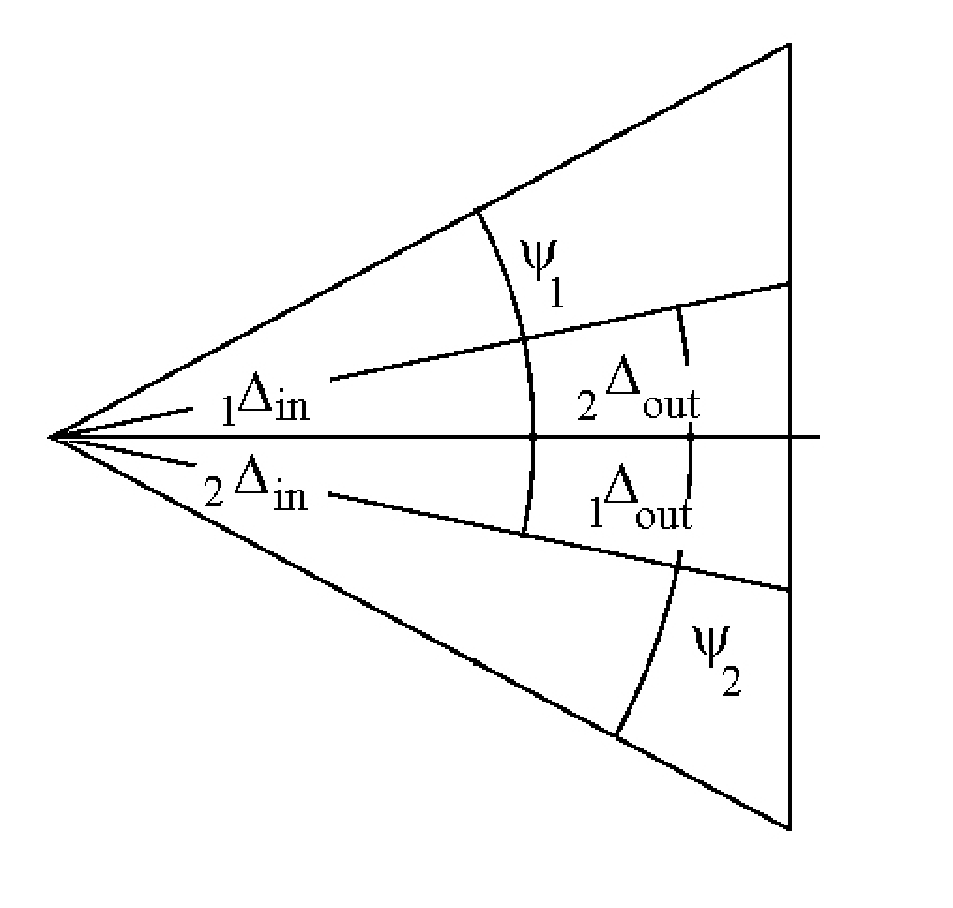
Now by construction

and (in view of the evolution of the null geodesics about the deflector)

so that

For an emitter at $u_{e}=0$ we have the rigorous result

Of particular note is the fact that for this configuration since $\Delta_{out}$ cancels out, $\Lambda$ plays no role, and further, the usual approximate argument gives the rigorously correct answer up to numerical evaluation.

More generally, when the associated $u_{{}_{\Sigma}}$ are not equal, but we continue to consider opposed sources and set $u_{e}=0$,

where the $\phi(0)$ are given by (12) and the $\chi$ by (20). Whereas $\Lambda$ does not enter the first term, it does not cancel from the second except in the limit ${}_{1}u_{\Sigma}=\;_{2}u_{\Sigma}$ which reproduces (32).

When the associated $u_{{}_{\Sigma}}$ are not equal, and the sources are not opposed, the differential deflection becomes

where again the $\phi(0)$ are given by (12) and the $\chi$ by (20) and we have taken $u_{e}=0$. Whereas $\Lambda$ does not enter the first term, it does not cancel from the second except in the limit ${}_{1}u_{\Sigma}=\;_{2}u_{\Sigma}$ which gives $\delta=0$ (we have one source).

The standard argument for explaining the measured value of the deflection of light is to set the emitter and observer at $u=0$ so that the total deflection for a single source for grazing incidence with the Sun is given by $(2\phi(0)-\pi)|_{u_{{}_{\bigodot}}}$, which, when approximated by first order corrections to the null geodesic equation, gives $4u_{{}_{\bigodot}}$ $(^{\prime\prime})$. For wide-angle deflections a similar argument leads to (27). On the basis of the mathematically exact solution to the classical bending problem I have shown that these are excellent approximations. However, as regards explaining the measured deflection of light, these approximate arguments fall short in the sense that the bending prior to and after an apse are fundamentally different. The post apsidal bending involves the process of measurement and is dominated by the cancelation of two terms, one of which is not considered in the usual approximate argument. Whereas these more involved arguments may not be numerically important, conceptually they are.

Aside form these details, the present discussion differs from others in the sense that analytic approximations to the exact solution (4) is not central to the discussion, as is the usual case, but rather (4) is viewed as an elementary function in the sense that it can be trivially approximated numerically to arbitrary accuracy using modern computational platforms. However, approximations have been included, relegated to the Appendices, as these serve to amplify and “explain” the results obtained.

References

- (1) Electronic Address: lake@astro.queensu.ca
- (2) W. Rindler and M. Ishak, Phys. Rev. D 76, 043006 (2007).
- (3) K. Lake, Phys. Rev. D 65, 087301 (2002).
- (4) The constancy of (as regards ), for grazing incidence, is set by junction conditions on the deflector as explained in lake. Since we have assumed that , the form (4) extends up to the condition that the null geodesic is observed at the apse. This is considered further below.
- (5) The fact that (3) can be solved exactly in terms of Elliptic integrals is well known. See, for example, S. Chandrasekhar, The Mathematical Theory of Black Holes, (Oxford Universirty Press, Oxford 1983). Whereas many works are primarily concerned with analytical approximations to (4), these are not of central concern here. See also G. V. Kraniotis, Class. Quantum Grav. 22, 4391 (2005).
- (6) For , and for , .
- (7) See, for example, Handbook of Mathematical Functions, Edited by M. Abramowitz and I. A. Stegun (Dover, New York, 1972) Section 17.4.17.
- (8) The limit plays a central role in most arguments and this limit deserves special consideration for . If the emitter lies within the cosmological horizon we have the restriction where for jhm. Using current limits on , for a solar mass deflector, we have . This does not change in any significant way any argument in this paper (but see Appendix B).
- (9) See, for example, M. J. Jaklitsch, C.Hellaby and D. R. Matravers, GRG 21 941 (1989) (Appendix I).
- (10) We use the following adopted values: , and . I report only 6 digit accuracy, whereas the calculations were done with 40 digit accuracy under Maple, assuming, of course, that the adopted values are defined to be exact to this degree. When viewing the Tables, one should be mindful of roundoff. In the real world, light deflection to 6 digit accuracy is of course influenced by other factors not considered here.
- (11) Let us note here that a few presentations do go beyond a consideration of (14) alone. These include C. M. Will, Theory and experiment in gravitational physics, (Cambridge University Press, Cambridge, 1993) and C. W. Misner, K. S. Thorne and J. A, Wheeler, Gravitation, (Freeman, San Francisco, 1973).
- (12) See C. M. Will, “The Confrontation between General Relativity and Experiment”, Living Rev. Relativity 9, (2006), 3. URL (cited on October 22, 2007): http://www.livingreviews.org/lrr-2006-3.
- (13) The text by B. O’Neill, Semi-Riemannian Geometry (Academic Press, New York, 1983) gives (20) for general given by (2). The text by M. Kriele, Spacetime (Springer, Berlin, 2001) gives the result for . Curiously, in neither case is related to which is calculated in these texts in the usual approximate way, .
- (14) The notation comes from the fact that the factor is exact.
- (15) Note that increases monotonically with distance even though this is not clear in the Table because of number. See also Appendix C.
- (16) For the planets I have used the semi-major axis.
- (17) It is, however, dificult to ignore the wonderful serendipity that Table 2 provides. For the Earth, is the date of the famous eclipse. Further, for the Earth, is the date before this eclipse when Astronomer Royal Sir F. W. Dyson first pointed out the opportunity afforded by this eclipse for verifying Einstein’s theory of gravitation (see F. W. Dyson, MNRAS 77, 445 (1917)).
- (18) See, S. S. Shapiro, J. L. Davis, D. E. Lebach and J. S. Gregory, Phys. Rev Lett. 92, 121101 (2004).
- (19) See I. I. Shapiro, Science 157, 806 (1967) and W. R. Ward, Ap. J. 162, 345 (1970).
- (20) This is sometimes referred to as “Eddington’s method”. See, for example, J. Plebański and A. Krasiński, General Relativity and Cosmology, (Cambridge University Press, Cambridge, 2006). Since we have restricted our analysis to , when we consider more than one source, the sources must be aligned radially through the centre of the deflector.
- (21) C. R. Keeton and A. O. Petters, Phys. Rev D 72 , 104006 (2005) arXiv:gr-qc/0511019v1
- (22) For recent discussions of lensing with see M. Ishak, W. Rindler, J. Dossett, J. Moldenhauer and C. Allison arXiv:0710.4726v1, M. Sereno arXiv:0711.1802v1 and P. Bakala, P. Cermak, S. Hledik, Z. Stuchlik and K. Truparova arXiv:0709.4274v1