Statistical Mechanical Models and Topological Color Codes

Let us start by recalling the notion of a Topological Color Code (TCC) in order to see what type of classical spin models we obtain from them with appropriate projections onto factorized quantum states and specific lattices.

A TCC, denoted by ${\cal C}$, is a quantum stabilizer error correction code constructed with certain class of two-dimensional lattices called 2-colexes. The word colex is a contraction that stands for color complex, where complex is the mathematical terminology for a rather general lattice homologicalerror. A 2-colex, denoted by $\mathfrak{C}_{2}$, is a 2D trivalent lattice which has 3-colorable faces and is embedded in a compact surface of arbitrary topology like a torus of genus $g$. A trivalent lattice is one for which three edges meet at every vertex. The property of being 3-colorable means that the faces (or plaquettes) of the lattice can be colored with these colors in such a way that neighboring faces never have the same color. We select as colors red (r), green (g) and blue (b). An example of a 2-colex construction is shown in Fig. 1.

Edges can be colored in according to the coloring of the faces. In particular, we attach red color to the edges that connect red faces, and so on and so forth for the blue and gree edges/faces. When studying higher dimensional colexes, it turns out that the coloring of the edges is the key property of $D$-colexes: all the information about a $D$-colex is encoded in its 1-skeleton, i.e., the set of edges with its coloringtopo3D.

Given a 2-colex $\mathfrak{C}_{2}$, a TCC ${\cal C}$ is constructed by placing one qubit at each vertice of the colored lattice. Let us denote by $\mathfrak{V}$, $\mathfrak{E}$ and $\mathfrak{F}$ the sets of vertices $\mathfrak{v}$, edges $\mathfrak{e}$ and faces $\mathfrak{f}$, respectively, of the given 2-colex. Then, the generators of the stabilizer group, denoted by ${\mathcal{S}}$, are given by face operators only. For each face $\mathfrak{f}$, they come into two types depending whether they are constructed with Pauli operators of $X$- or $Z$-type:

and there are no generators associated to lattice vertices. For example, an hexagonal lattice is an instance of a 2-colex, see Fig. 2. The operators for the face $\mathfrak{f}$ displayed in the figure take the form $X_{\mathfrak{f}}=X_{1}X_{2}X_{3}X_{4}X_{5}X_{6},Z_{\mathfrak{f}}=Z_{1}Z_{2}Z_{3}Z_{4}Z_{5}Z_{6}$.

A given state $|\Psi_{\rm c}\rangle\in{\cal C}$ is left trivially invariant under the action of the face operators,

An erroneous state $|\Psi\rangle_{\rm e}$ is one that violates conditions (2) for some set of face operators of either type. As the generator operators $X_{\mathfrak{f}},Z_{\mathfrak{f}}\in{{\mathcal{S}}}$ satisfy that they square to the identity operator, $(X_{\mathfrak{f}})^{2}=1\hskip-2.5pt{\rm I}=(Z_{\mathfrak{f}})^{2},\forall\mathfrak{f}\in\mathfrak{F}$, then an erroneous state is detected by having a negative eigenvalue with respect to some set of stabilizer generators: $X_{\mathfrak{f}}|\Psi\rangle_{\rm e}=-|\Psi\rangle_{\rm e}$ and/or $Z_{\mathfrak{f}}|\Psi\rangle_{\rm e}=-|\Psi\rangle_{\rm e}$.

Interestingly enough, it is possible to construct a quantum lattice Hamiltonian $H_{\rm c}$ such that its ground state is degenerate and corresponds to the TCC ${\cal C}$, while the erroneous states are given by the spectrum of excitations of the Hamiltonian topodistill. Such Hamiltonian is constructed out of the generators of the topological stabilizer group ${\mathcal{S}}$,

The ground state of this Hamiltonian exhibits what is called a topological order wenbook04, as opposed to a more standard order based on an spontaneous symmetry breaking mechanism. One of the signatures of that topological order is precisely the topological origin of the ground state degeneracy: the number of degenerate ground states depends on topological invariants like Betti numbers topo3D. In two dimensional lattices, the relevant Betti number corresponds to the Euler characteristic $\chi$ of the surface where the 2-colex is embedded.

In order to better understand both the ground state and excitations of this Hamiltonian and their topological properties, it is rather convenient to introduce the set of string operators that can be defined on a 2-colex $\mathfrak{C}_{2}$. String operators are generalizations of face operators (1) that can be either open or closed, i.e., with or without end-points. These strings are topological and like in Kitaev model, the homology is defined on $\mathbf{Z}_{2}$ since we work with two-level quantum systems located at the sites of the lattice. However, in a TCC we have an additional ingredient to play around: color. Let us split the sets of edges and faces into colored subsets denoted by $\mathfrak{E}:=\mathfrak{E}_{r}\cup\mathfrak{E}_{g}\cup\mathfrak{E}_{b}$ and $\mathfrak{F}:=\mathfrak{F}_{r}\cup\mathfrak{F}_{g}\cup\mathfrak{F}_{b}$, where $\mathfrak{E}_{r}$ is the subset of red edges, and similarly for the rest of subsets.

A colored string $\gamma$ is a collection of edges of a given color. Thus, a blue string $\gamma$ takes the form $\gamma=\{e_{i}\}$ with $e_{i}\in\mathfrak{E}_{b}$. The definition of colored string operators is completely analogous to that of face operators:

where, in turn, $X_{\mathfrak{e}}=X_{\mathfrak{v}_{1}}\otimes X_{\mathfrak{v}_{2}}$ if $\mathfrak{v}_{1}$ and $\mathfrak{v}_{2}$ are the sites at the ends of the edge $\mathfrak{e}$, and similarly for $Z_{\mathfrak{e}}=Z_{\mathfrak{v}_{1}}\otimes Z_{\mathfrak{v}_{2}}$. For instance, consider the red string operator in Fig. 2, where we have $X_{\gamma}=X_{a}X_{b}X_{c}X_{d}X_{e}X_{f}\cdots,Z_{\gamma}=Z_{a}Z_{b}Z_{c}Z_{d}Z_{e}Z_{f}\cdots$.

Colored strings are open if they have endpoints. These endpoints are localized at faces which share color with the string. In particular, a face $\mathfrak{f}$ is an endpoint of $\gamma$ if the number of edges of $\gamma$ meeting at $\mathfrak{f}$ is odd, see Fig. 2. In terms of string operators, a face $\mathfrak{f}$ is an endpoint of $\gamma$ if $\{X_{\gamma},Z_{\mathfrak{f}}\}=0$ or, equivalently, if $\{Z_{\gamma},X_{\mathfrak{f}}\}=0$. Thus, open string operators do not commute with those face operators in their ends. In other words, a string operator that commutes with all the face operators must correspond to a closed string, that is, a string without endpoints. In terms of the Hamiltonian (3), string operators produce quasi-particle excitations at their ends when applied to the ground state. These quasi-particle excitations are Abelian anyons.

Closed strings are mainly of two types. They can be homologically trivial, meaning that they are the boundary of certain area of the surface, or homologically nontrivial. In terms of operators, a string is a boundary iff its string operators belong to the stabilizer group ${\mathcal{S}}$ of the color code $\cal C$. Such boundary string operators are thus products of face operators. In fact, face operators themselves are the basic boundary string operators.

Although we have introduced colored strings and the corresponding operators for illustrative purposes, in fact in a TCC we have to deal with more general objects, namely string-nets. A string-net is a collection of strings meeting at certain branching or ramification points. An example of these types of configurations are shown in Fig. 3.

A string-net $\gamma$ is a collection of vertices $\gamma\subset\mathfrak{V}$. Equivalently, $\gamma$ is a formal sum of lattice vertices $\mathfrak{v}\in\mathfrak{V}$ with coefficients $\gamma_{\mathfrak{v}}\in\mathbf{Z}_{2}$, i.e.,

where $\gamma_{\mathfrak{v}}=1$ if $\mathfrak{v}\in\gamma$ and $\gamma_{\mathfrak{v}}=0$ otherwise. Given a string-net $\gamma$, we define the string-net operators

Just as in the case of colored strings, we can talk about open and closed string-nets, and about trivial and non-trivial closed string-nets. In terms of operators, the situation is exactly the same as with strings. That is, a string-net $\gamma$ has an endpoint at a face $\mathfrak{f}$ if $\{X_{\gamma},Z_{\mathfrak{f}}\}=0$, it is closed if its string-net operators commute with all the face operators, and it is a boundary if it is a product of face operators. In order to translate these ideas into purely geometric terms, we can define the boundary operator

where $|\gamma\cap\mathfrak{f}|$ is the number of vertices that $\gamma$ and $\mathfrak{f}$ share. Thus $\partial_{c}\gamma$ is the formal sum of the endpoints of $\gamma$. It is also natural to define an operator $\partial_{c}$ for faces

so that $\partial_{c}\mathfrak{f}$ is the string-net composed of the vertices of $\mathfrak{f}$. With this definitions, $\gamma$ is closed if and only if

and it is a boundary if and only if there exist a collection of faces $S=\sum_{\mathfrak{f}}S_{\mathfrak{f}}\mathfrak{f}$ such that

It is possible to give explicit expressions for the states of the TCC or, equivalently, for the ground states of the Hamiltonian (3). The states are superpositions of all possible closed string-nets, a typical feature of the ground states of systems with topological order wenbook04, levinwen05. The following is an un-normalized ground state for any given 2-colex topodistill, topo3D

where $|\mathfrak{V}|$ is the number of vertices in the 2-colex $\mathfrak{C}_{2}$, $\Gamma_{0}$ denotes the set of boundary string-nets and $|0\rangle$ is the eigenstate $Z|0\rangle=|0\rangle$.

The degeneracy of the ground state or, equivalently, the number of logical states encoded in the color code, depends on the topology of the lattice. For a general 2-colex $\mathfrak{C}_{2}$ with Euler characteristic $\chi(\mathfrak{C}_{2}):=|\mathfrak{V}|-|\mathfrak{E}|+|\mathfrak{F}|$, the number $k$ of encoded qubits is given by $k=4-2\chi(\mathfrak{C}_{2}):=2h_{1}$ topodistill, where $h_{1}$ is the first Betti number of the surface where the 2-colex is embedded topo3D. These additional ground states can be obtained from the one given by (11) by the action of the encoded logical operators $\bar{X}_{i},\bar{Z}_{i}$ with $i=1,\ldots,k$. These, in turn, take the form of string-net operators of non-trivial closed string-nets topodistill.

For the purpose of this work, we shall be interested only in a representative ground state like (11). Thus, we will have to consider suitable surface topologies such that the corresponding TCC is unique. We will return over this issue later when we consider particular lattices.

Now, we come to the issue of what type of classical spin models may arise from the color code state (11) when we project it onto a product state of a number of qubits given by $|\mathfrak{V}|$. In this section we shall not consider the most general factorized state, but one specifically adapted for the purpose of this connection in its most simple form, namely,

with $\beta:=1/k_{\rm B}T$ the inverse temperature parameter.

The classical spin model arises when computing the overlapping between the ground state of the color code Hamiltonian (11) and this factorized state (12),

Using (11) and (12) we get the following expression for this overlapping,

$u:=\tanh(\beta J)$ and $|\gamma|$ is the number of vertices of $\gamma$.

We want to relate (14) to the partition function of a classical spin system. So let $\mathfrak{C}_{2}$ be an arbitrary 2-colex. Consider the dual lattice $\Lambda$. The vertices of $\Lambda$ correspond to the faces of $\mathfrak{C}_{2}$, and the faces of $\Lambda$ are vertices in $\mathfrak{C}_{2}$. In particular, $\Lambda$ is a lattice in which all faces are triangular and vertices are 3-colorable. Moreover, for any such lattice $\Lambda$ there exist a suitable dual 2-colex $\mathfrak{C}_{2}$.

So let us associate a classical system to $\Lambda$ by attaching classical spin variables $\sigma_{i}=\pm 1$ to each of its sites $i$ (equivalently, to each face $\mathfrak{f}$ of $\mathfrak{C}_{2}$). The classical Hamiltonian is

where $J$ is a coupling constant and the sum $\sum_{\langle i,j,k\rangle}$ is over all triangles with spins $\sigma_{i}\sigma_{j}\sigma_{k}$ at their vertices. Thus, we have a classical Ising model with 3-body interactions. The case $J>0$ corresponds to a ferromagnetic model with an even parity to be discussed below, and similarly $J<0$ to an antiferromagnetic model with odd parity. The partition function of the model is

where the sum $\sum_{\{\sigma\}}$ is over all possible configurations of spins. The point then is that we have

where $N$ is the number of sites.

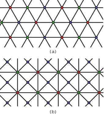
Before we show why this identity holds, let us give a pair of representative examples of dual lattices $\mathfrak{C}_{2}$ and $\Lambda$. First, if the 2-colex is an hexagonal lattice then the dual lattice $\Lambda$ is a triangular lattice, Fig. 4(a). Second, if the 2-colex is a square-octogonal lattice (also denoted by 4-8 lattice), then its dual is a Union Jack lattice, see Fig. 4(b). The relevance of these examples is two-fold. On the one hand, the hexagonal lattice is the simplest lattice for a 2-colex and the 4-8 lattice is the simplest one when we want to obtain TCC with certain transversality properties for quantum computation (see below). On the other hand, 3-body classical Ising-models on both lattices have been studied in statistical mechanics to some extent.

To prove (17), let us start expanding the partition function ${\cal Z}(\beta J)$ (16) using the following identity,

Inserting it into (16), we may expand the partition function as

Let us rewrite (45) in the form

where $\delta=\sum_{\langle i,j,k\rangle}\delta_{ijk}\triangle_{ijk}$ is a chain of triangles, that is, a formal sum over triangles with binary coefficients, and $|\delta|$ is the number of triangles in $\delta$. Using the identities

where $n_{o}$ and $n_{e}$ are odd and even numbers, respectively, we get

where $\Delta_{0}$ contains those chains of triangles such that at any given site $i$ an even number of triangles meet, as shown in Fig. 5. In fact, this type of expansion is called a high-temperature expansion of the partition function of a statistical mechanical model newell_montroll_53.

In order to compare (40) and (52), we simply observe that triangles $\triangle_{ijk}$ in $\Lambda$ correspond to vertices of the 2-colex $\mathfrak{v}\in\mathfrak{V}$. This correspondence relates in an obvious way a string-net $\gamma$ with a triangle chain $\delta$, in such a way that $\Delta_{0}$ is identified with $\Gamma_{0}$. Therefore, we have the desired relationship between the overlapping and the partition function (17).

Although the previous derivation was performed for a model with uniform couplings, it is possible to obtain a completely analogous result for triangle dependent couplings $J_{ijk}$. For simplicity we have preferred to do the exposition with uniform couplings because, in fact, the case of non-uniform couplings is contained in the more general case of non-uniform couplings with non-uniform external field, to be considered in section V.

We hereby draw a series of very important consequences from these results, that will continue in the next section.

Remarkably, the gauge group underlying the topological order related to Hamiltonian (3) is also $\mathbf{Z}_{2}\times\mathbf{Z}_{2}$. The situation is the same also with toric codes, where the global symmetry of the classical system is $\mathbf{Z}_{2}$ and the gauge group for the toric code topological order is $\mathbf{Z}_{2}$. This is certainly not a matter of chance, since one can relate the types of domain walls in the classical system to the types of condensed strings in the quantum system.

Duality is a property between high-temperature and low-temperature expansions of a statistical mechanical model like (16) or (23). A high-temperature expansion is a polynomial in the variable $u=\tanh(\beta J)$ that is small when $T\rightarrow\infty$, while a low temperature expansion is another polynomial in the variable $u^{\ast}:={\rm e}^{-2\beta J^{\ast}}$ that is small in the limit $T\rightarrow 0$. Then, a self-duality is a relationship between the high-temperature expansion of one classical spin model in a given lattice $\Lambda$ and the low-temperature expansion of the same lattice. This is precisely the case of the 3-body Ising model (16) on both the triangular and Union Jack lattices wood_g_72, merlini_gruber_72 and the standard Ising model (23) krammers_wannier_41.

The critical exponent for the specific heat in the 3-body Ising model on the triangular lattice is $\alpha=\frac{2}{3}$. This represents a power law behaviour which is in sharp contrast with the well-known logarithmic divergence ($\alpha=0$) of the specific heat in the standard Ising model (23). Other representative exponents are also different: the correlation length exponent is $\nu=\frac{2}{3}$ (vs. $\nu=1)$, the magnetization exponent is $\beta=\frac{1}{12}$ (vs. $\beta=\frac{1}{8}$), while they share the same two-point correlation function exponent at the critical point $\eta=\frac{1}{4}$.

For the 3-body Ising model on the Union Jack lattice, the specific heat critical exponent is also remarkably different $\alpha=\frac{1}{2}$. In fact, if the coupling constant $J$ is allowed to be anisotropic, then even the critical exponent $\alpha$ may take on a set of continuous values in $(0,\frac{1}{2})$ depending on a parameter related to the coupling constants h_m_72.

The computational capabilities of a topological color code depends on the 2-colex lattices where it is defined. For a TCC on a square-octogonal lattice it is possible to implement the whole Clifford group of unitary gates generated by the set of gates $\{H,K^{\frac{1}{2}},\Lambda_{2}\}$, where $H$ is the Hadamard gate, $K^{\frac{1}{2}}$ the $\pi/8$-gate and $\Lambda_{2}$ the CNOT gate topodistill. However, for a 2-colex like the hexagonal lattice the set of available gates is more reduced since the $\pi/8$-gate cannot be implemented topologically topodistill. Thus we point out a remarkable connection between different computational capabilities of color codes that correspond to qualitatively different unversality classes of their associated classical spin models, despite the fact that both color codes have the same topological order.

If we want to consider classical systems of spins with a finite number of sites, then we have to introduce either borders or a nontrivial topology. Since in TCCs the nontrivial topology gives rise to degeneracy, it is preferable to have borders. Also, borders play a role for the ideas to be explained in the next section.

In TCCs, borders can be of several types. For example, in topodistill it was shown how to build borders of a given color. Here our guide to construct the border must be the dual lattice $\Lambda$, which now has a border, along with the properties of the classical system. Then, as shown in Fig. 6, in order to construct the stabilizer for a TCC with border in such a way that (17) remains true is to start with an infinite 2-colex $\mathfrak{C}_{2}$ and then keep only part of it following certain criteria. (i) Keep those vertices $\mathfrak{v}$ of $\mathfrak{C}_{2}$ which correspond to triangles in $\Lambda$. (ii) For those faces $\mathfrak{f}$ of $\mathfrak{C}_{2}$ which keep all their vertices, we keep the face operators $X_{\mathfrak{f}}$ and $Z_{\mathfrak{f}}$. (iii) For those faces $\mathfrak{f}$ which only keep a subset $\mathfrak{f}^{\prime}$ of their vertices, we introduce a face operator $Z_{\mathfrak{f}^{\prime}}$ acting on those qubits. Condition (i) ensures the correspondence between triangle chains in $\Lambda$ and string-nets in $\mathfrak{C}_{2}$. Conditions (ii) and (iii) ensure the correspondence between $\Gamma_{0}$ and $\Delta_{0}$.

Instead of giving a general definition of cluster states, we will consider only bipartite cluster states. So let $\mathfrak{G}$ be a finite bipartite graph, that is, a graph such that its set of vertices $\mathfrak{U}$ is the disjoint union of two sets $\mathfrak{U}=\mathfrak{U}_{1}\cup\mathfrak{U}_{2}$ in such a way that neighboring vertices never belong to the same $\mathfrak{U}_{i}$. Consider the quantum system obtained by attaching a qubit to each of the vertices $\mathfrak{u}$. For each such vertex, we denote by $N(\mathfrak{u})$ the set containing both $\mathfrak{u}$ and its neighbors. The cluster state $|\kappa\rangle$ for the graph $\mathfrak{G}$ is then completely characterized by the conditions:

In order to relate the TCC $\mathcal{C}$ of a 2-colex $\mathfrak{C}_{2}$ to a cluster state, we construct a bipartite graph $\mathfrak{G}$ by setting $\mathfrak{U}_{1}=\mathfrak{V}$ and $\mathfrak{U}_{2}=\mathfrak{F}$. Then the edges are defined so that $\mathfrak{u}_{1}=\mathfrak{v}\in\mathfrak{U}_{1}$ is a neighbor of $\mathfrak{u}_{2}=\mathfrak{f}\in\mathfrak{U}_{2}$ if $\mathfrak{v}$ is a vertex of $\mathfrak{f}$ in $\mathfrak{C}_{2}$, see Fig. 7. Observe that the corresponding cluster state $|\kappa\rangle$ satisfies

because $X_{\mathfrak{f}}=\bigotimes_{\mathfrak{v}\in\mathfrak{f}}X_{N(\mathfrak{v})}$. In fact, if $\gamma$ is a string-net with $\partial_{c}\gamma=0$, then $X_{\gamma}|\kappa\rangle=|\kappa\rangle$. However, to keep things as simple as possible, let us just consider 2-colexes in which all closed string-nets are boundaries. If we measure in the $Z$ basis all the qubits corresponding to vertices $\mathfrak{u}\in\mathfrak{U}_{2}$ we will obtain a series of binary values $x_{\mathfrak{u}}=x_{\mathfrak{f}}$. The remaining qubits are then in a state characterized by the conditions:

Thus, if $x_{\mathfrak{f}}=0$ for all the faces $\mathfrak{f}$, the result is the TCC state $|\Psi_{\rm c}\rangle$ (11). In the other cases the result is essentially a TCC, in particular the state is

where $\boldsymbol{\mathrm{x}}$ denotes the binary vector of the measurement results and $\Gamma_{\boldsymbol{\mathrm{x}}}$ is the set of string-nets $\gamma$ with $\partial_{c}\gamma=\sum_{\mathfrak{f}}x_{\mathfrak{f}}\mathfrak{f}$.

In fact, the original cluster state can be written as follows:

where $|\boldsymbol{\mathrm{x}}\rangle=\bigotimes_{\mathfrak{u}\in\mathfrak{U}_{2}}|x_{\mathfrak{u}}\rangle_{\mathfrak{u}}$ is an element of the computational basis of the subsystem of qubits in $\mathfrak{U}_{2}$. To check that this is indeed the correct expression for the cluster state, it is enough to note that it satisfies (V.1).

Thus far, we have only considered statistical mechanical models with zero external magnetic field. Here we go beyond that situation, considering the formulation of models with 3-body Ising interactions and arbitrary magnetic fields from the projection of topological color codes onto appropriate product states.

Let us define the product state

where $\boldsymbol{\mathrm{J}}=(J_{\mathfrak{v}})\in\mathbf{R}^{|\mathfrak{V}|}$, $\boldsymbol{\mathrm{h}}=(h_{\mathfrak{f}})\in\mathbf{R}^{|\mathfrak{F}|}$ and

Consider the overlapping

Its value is

where

We want to relate (39) to the partition function of a classical spin system. As in section III, we consider the lattice $\Lambda$ dual to the 2-colex $\mathfrak{C}_{2}$ and we associate a classical system to $\Lambda$ by attaching classical spin variables $\sigma_{i}=\pm 1$ to each of its sites $i$. This time however we include triangle dependent couplings $J_{ijk}$ in triangles and a site dependent external field $h_{i}$. Thus, we want to derive the high temperature expansion for the partition function

where the classical Hamiltonian is

We start using the identities

so that,

where

Let us rewrite (45) in the form

where $\boldsymbol{\mathrm{x}}=(x_{i})$ is a binary vector and $\delta=\sum_{\langle i,j,k\rangle}\delta_{ijk}\triangle_{ijk}$ is a chain of triangles, that is, a formal sum over triangles with binary coefficients. Reordering the expression we get

where

From (21) it follows that

where $\langle j,k\rangle_{i}$ denotes the pairs $(j,k)$ which form a triangle with $i$, and $N$ is the number of sites. Finally we can give the desired high temperature expansion of the partition function:

where $\Delta_{\boldsymbol{\mathrm{x}}}$ contains those chains of triangles such that at any given site $i$ an even (odd) number of triangles meet if $x_{i}=0$ ($x_{i}=1$).

In order to compare (40) and (52), we first observe that sites $i$ correspond to faces of the 2-colex $\mathfrak{f}\in\mathfrak{F}=\mathfrak{U}_{2}$ and triangles $\triangle_{ijk}$ correspond to vertices of the 2-colex $\mathfrak{v}\in\mathfrak{V}=\mathfrak{U}_{1}$. This correspondence relates in an obvious way $x_{i}$ with $x_{\mathfrak{v}}$, $h_{i}$ with $h_{\mathfrak{v}}$ and so on and so forth. Also, there is an exact correspondence between chains of triangle $\delta$ and string-nets $\gamma$. In particular, this correspondence identifies $\Delta_{\boldsymbol{\mathrm{x}}}$ with $\Gamma_{\boldsymbol{\mathrm{x}}}$, so that we get the desired relationship between the overlapping and the partition function

References

- (1) M. Van den Nest, W. Dür, and H. J. Briegel, “Classical Spin Models and the Quantum-Stabilizer Formalism”; Phys. Rev. Lett. 98, 117207 (2007); arXiv:quant-ph/0610157.
- (2) S. Bravyi and R. Raussendorf, “Measurement-based quantum computation with the toric code states”; Phys. Rev. A 76, 022304 (2007); arXiv:quant-ph/0610162.
- (3) A. Yu. Kitaev, “Fault-tolerant quantum computation by anyons”, Annals of Physics 303 no. 1, 2–30 (2003), quant-ph/9707021.
- (4) E. Dennis, A. Kitaev, A. Landahl, J. Preskill, “Topological quantum memory”. J. Math. Phys. 43, 4452-4505 (2002).
- (5) R. Raussendorf and H.-J. Briegel, “A One-Way Quantum Computer”, Phys. Rev. Lett. 86, 5188 (2001).
- (6) Hans J. Briegel and Robert Raussendorf, ”Persistent Entanglement in Arrays of Interacting Particles”; Phys. Rev. Lett. 86, 910 (2001).
- (7) M. Van den Nest, W. Dür, and H. J. Briegel, “Completeness of the classical 2D Ising model and universal quantum computation”; arXiv:0708.2275.
- (8) H. Bombin and M. A. Martin-Delgado; “Topological Quantum Distillation”; Phys. Rev. Lett. 97, 180501 (2006); quant-ph/0605138.
- (9) H. Bombin and M.A. Martin-Delgado; “Topological Computation without Braiding”; Phys. Rev. Lett. 98, 160502 (2007); quant-ph/0610024.
- (10) H. Bombin and M.A. Martin-Delgado “Exact Topological Quantum Order in D=3 and Beyond: Branyons and Brane-Net Condensates”; Phys. Rev. B 75, 075103 (2007); cond-mat/0607736.
- (11) H. Bombin and M.A. Martin-Delgado; “Homological Error Correction: Classical and Quantum Codes”; J. Math. Phys. 48, 052105 (2007); quant-ph/0605094.
- (12) X.-G. Wen. Quantum Field Theory of Many-body Systems, Oxford University Press, (2004).
- (13) M. Levin and X.-G. Wen, “String-net condensation: A physical mechanism for topological phases”. Phys. Rev. B 71, 045110 (2005).
- (14) H. Bombin and M.A. Martin-Delgado; “Optimal Resources for Topological 2D Stabilizer Codes: Comparative Study”, Phys. Rev. A 76, 012305 (2007); quant-ph/0703272.
- (15) D. Gottesman, “Class of quantum error-correcting codes saturating the quantum Hamming bound”. Phys. Rev. A 54, 1862 (1996).
- (16) G.F. Newell and E.W. Montroll, “On the Theory of the Ising Model of Ferromagnetism”; Rev. Mod. Phys. 25, 353 (1953).
- (17) R.J. Baxter and F.Y. Wu; “Exact Solution of an Ising Model with Three-Spin Interactions on a Triangular Lattice”; Phys. Rev. Lett. 31, 1294 (1973).
- (18) R.J. Baxter and F.Y. Wu; “Ising Model on a Triangular Lattice with Three-Spin Interactions. The eigenvalue equation”; Aust. J. Phys. 27, 357 (1974).
- (19) A. Hintermann and D. Merlini, “Exact Solution of a Two Dimensional Ising Model with Pure 3 Spin Interactions”, Phys. Lett. A 41, 208 (1972).
- (20) H.A. Krammers and G.H. Wannier, “Statistics of the Two-Dimensional Ferromagnet. Part I”; Phys. Rev. 60, 252 (1941).
- (21) D.W. Wood and H.P. Griffiths, “A Self Dual Relation for an Ising Model with Triplet Interactions”; J. Phys. C: Solid State Phys. 5 L253 (1972).
- (22) D. Merlini and C. Gruber, “Spin-1/2 Lattice System: Group Structure and Duality Relation”; J. Math. Phys. 13 1814 (1972).
- (23) F. Barahona, “On the computational complexity of Ising spin glass models”, J. Phys. A: Math. Gen. 15, 3241 (1982).
- (24) P. Kasteleyn, “The statistics of dimers on a lattice, I. The number of dimer arrangements on a quadratic lattice”, Physica 27, 1209 (1961).
- (25) E. Rico and H.J. Briegel, “2D Multipartite Valence Bond States in Quantum Antiferromagnets”; arXiv:0710.2349.