跳到论文正文
W Papers独立论文阅读器 arXiv:0711.0432 论文正文 计算阅读时间 · 0%
引用这篇论文根据当前论文元数据生成,正式投稿前建议核对。


License: Assumed arXiv.org perpetual non-exclusive license
arXiv:0711.0432v2 [hep-ph] 08 Nov 2007

Radiative charmless B(s)→V​γB_{(s)}\to V\gamma and B(s)→A​γB_{(s)}\to A\gamma decays in pQCD approach

Wei Wanga, Run-Hui Lib,a and Cai-Dian Lüa Affiliation: a Institute of High Energy Physics, P.O. Box 918(4) Beijing 100049, P.R. China
b Department of Physics, Shandong University, Jinan 250100, P.R. China
c Graduate University of Chinese Academy of Sciences, Beijing 100049, P.R. China
Abstract

We study the radiative charmless B(s)→V⁡(A)​γB_{(s)}\to V(A)\gamma decays in perturbative QCD (pQCD) approach to the leading order in αs\alpha_{s} (here VV and AA denotes vector mesons and two kinds of axial-vector mesons: P13{}^{3}P_{1} and P11{}^{1}P_{1} states, respectively.). Our predictions of branching ratios are consistent with the current available experimental data. We update all B(s)→VB_{(s)}\to V form factors and give the predictions for B→AB\to A form factors using the recent hadronic inputs. In addition to the dominant factorizable spectator diagrams, which is form factor like, we also calculate the so-called “power suppressed” annihilation type diagrams, the gluonic penguin, charming penguin, and two photon diagrams. These diagrams give the main contributions to direct CP asymmetries, mixing-induced CP asymmetry variables, the isospin asymmetry and U-spin asymmetry variables. Unlike the branching ratios, these ratios or observables possess higher theoretical precision in our pQCD calculation, since they do not depend on the input hadronic parameters too much. Most of the results still need experimental tests in the on-going and forthcoming experiments.

I Introduction

Present studies on BB decays are mainly concentrated on the precise test of standard model (SM) and the search for signals of possible new physics. Radiative processes b→s​γb\to s\gamma and b→d​γb\to d\gamma are among the most ideal probes and thus have received considerable efforts Hurth:2003vb. In the standard model, these processes are induced by the flavor-changing-neutral-current transitions which are purely loop effects. Such decays are rare and the measurement of parameters in these channels, especially the CP asymmetry variables, may shed light on detailed information on the flavor structure of the electroweak interactions. This predictive power relies on the accuracy of both the experimental side and the theoretical side. Thanks to the technique of operator-product-expansion, remarkable theoretical progress has been made in the SM to the next-to-next-to-leading order accuracy Misiak:2006zs. Compared with experimental results Barberio:2006bi, the theoretical prediction is consistent with but 1.2​σ1.2\sigma below the experimental data Hurth:2007xa. This consistence could certainly provide a rather stringent constraint on non-standard model scenarios.

Compared with inclusive processes, the exclusive processes B→V​γB\to V\gamma is more tractable on the experimental side, but more difficult on the theoretical side. Theoretical predictions are often hampered by our ability to calculate the decay amplitude ⟨V​γ​|Oi|​B⟩\langle V\gamma|O_{i}|B\rangle, where OiO_{i} is a magnetic moment or a four-quark operator. We have to use some non-perturbative hadronic quantities to describe the bound state effects. In the heavy-quark limit, the non-perturbative contributions can be organized in a universal and channel-independent manner. Factorization analysis, the separation of the short-distance and long-distance dynamics, can give many important predictions.

The dominant contribution to the radiative decay amplitudes is proportional to the transition form factor. Different treatments on the dynamics in form factor FB→VF^{B\to V} result in different explicit approaches. There are many approaches such as Lattice QCD (LQCD) DelDebbio:1997kr, light-front quark model (LFQM) Cheng:2003sm; Cheng:2004yj and light-cone sum rules (LCSR) Ball:2004rg. Recently three commonly-accepted approaches are developed to study exclusive BB decays: QCD factorization (QCDF) Beneke:1999br, soft collinear effective theory (SCET) Bauer:2001cu and perturbative QCD approach Keum:2000ph. In pQCD approach, the recoiling meson moves on the light-cone and a large momentum transfer is required. Keeping quarks’ transverse momentum, pQCD approach is free of endpoint divergence and the Sudakov formalism makes it more self-consistent. It has been successfully applied to various decay channels and quite recently this approach is accessing to next-to-leading order accuracy Nandi:2007qx. A bigger advantage is that we can really do the form factor calculation and the quantitative annihilation type diagram calculation in this approach. The importance of annihilation diagrams are already tested in the predictions of direct CP asymmetries in B0→π+​π−B^{0}\to\pi^{+}\pi^{-}, K+​π−K^{+}\pi^{-} decays Keum:2000ph; direct and in the explanation of B→ϕ​K∗B\to\phi K^{*} polarization problem kphi; kphi-e. These “power suppressed” contributions are the main source of isospin symmetry breaking (or SU(3) breaking) effects in radiative decays B→V​γB\to V\gamma Keum:2004is; Lu:2005yz.

Some of charmless B→V​γB\to V\gamma decay channels have been studied in pQCD approach Keum:2004is; Lu:2005yz; Li:2006xe separately. According to the transition at the quark level, all the 10 decay channels can be divided into three different groups: b→sb\to s, b→db\to d and purely annihilation type. The two B→K∗​γB\to K^{*}\gamma modes (b→sb\to s process) have been well measured experimentally. The agreement of pQCD approach results and experimental data Barberio:2006bi is very encouraging. In this paper, we study all those channels including the corresponding BsB_{s} decays in a comprehensive way. The input hadronic parameters will be chosen the same as that in Ref. Ali:2007ff. We also updated all the B→VB\to V decay form factors in pQCD approach Lu:2002ny. Despite branching ratios and CP asymmetry parameters which heavily depend on the input parameters, we also study some ratios characterizing the isospin and SU(3) breaking effects, where most of the uncertainties cancel. Experimental measurements of these quantities will prove a good test of our theory, since different method gives different prediction. With the ongoing BB factories BaBar and Belle, the BB-Physics program on CDF and the onset of the LHC experiments, as well as the Super B-factories being contemplated for the future, we expect a wealth of data involving these decays.

Although experimentalists have already measured one channel of the B→A​γB\to A\gamma decays Abe:2004kr, there are not many discussions on the theoretical side. The pQCD study on B→V​γB\to V\gamma can be straightforward extended to radiative processes involving higher resonants such as K1​(1270)K_{1}(1270), K1​(1400)K_{1}(1400). In the quark model, the quantum numbers JP​CJ^{PC} for the orbitally excited axial-vector mesons are 1+⁣+1^{++} or 1+⁣−1^{+-}, depending on different spins of the two quarks. In SU(3) limit, these mesons can not mix with each other; but since the ss quark is heavier than u,du,d quarks, K1​(1270)K_{1}(1270) and K1​(1400)K_{1}(1400) are not purely 13​P11^{3}P_{1} or 11​P11^{1}P_{1} states. These two mesons are believed to be mixtures of K1​AK_{1A} and K1​BK_{1B}, where K1​AK_{1A} and K1​BK_{1B} are P13{}^{3}P_{1} and P11{}^{1}P_{1} states, respectively. In general, the mixing angle can be determined by experimental data. But unfortunately, there is not too much data on the mixing of these mesons which leaves the mixing angle much free. Analogous to η\eta and η′\eta^{\prime}, the flavor-singlet and flavor-octet axial-vector meson can also mix with each other. Using those hadronic parameters determined in B→V​γB\to V\gamma decays, the production of A​γA\gamma in BB decays could provide a unique insight to these mysterious axial-vector mesons.

This paper is organized as follows: In section II, we briefly review pQCD approach with the operator basis used subsequently. Some input quantities which enter pQCD approach, wave function of the BB-meson, distribution amplitudes for light vector mesons, and for light axial-vector mesons and input values of the various mesonic decay constants, are also given here. In section III, we give the factorization formulae and the numerical results for B→VB\to V and B→AB\to A form factors. Section IV contains the calculation of B→V​γB\to V\gamma decays, making explicit the contributions from the electromagnetic diploe operator, the chromo-magnetic moment operator, some higher order (𝒪⁡(αs){\cal O}(\alpha_{s})) corrections from tree operators, the contribution from two-photon diagrams, the tree operator annihilation diagrams and penguin operator annihilation diagrams. Numerical results for the charge-conjugated averages of decay branching ratios are given in comparison with the corresponding numerical results obtained in QCDF approach and SCET, as well as the available experimental data. We also give direct CP-asymmetries, time-dependent CP asymmetries SfS_{f} and observables HfH_{f} (for BsB_{s} system) in the time-dependent decay rates in this section. In section V, we study B→A​γB\to A\gamma decays by predicting branching ratios and direct CP asymmetries. Our summary is given in the last section. Some functions are relegated to the appendix: appendix A contains the various functions that enter the factorization formulae in the pQCD approach; appendix B and C give the analytic formulae for the B→V​γB\to V\gamma and B→A​γB\to A\gamma decays used in numerical calculations, respectively.

II Formalism of pQCD approach

II.1 Notations and conventions

We specify the weak effective Hamiltonian which describes b→Db\to D (D=d,sD=d,s) transitions Buchalla:1995vs:

ℋe​f​f\displaystyle{\cal H}_{eff} =\displaystyle= GF2{∑q=u,cVq​bVq​D∗[C1(μ)O1q(μ)+C2(μ)O2q(μ)]\displaystyle\frac{G_{F}}{\sqrt{2}}\bigg\{\sum\limits_{q=u,c}V_{qb}V_{qD}^{*}\big[C_{1}({\mu})O^{q}_{1}({\mu})+C_{2}({\mu})O^{q}_{2}({\mu})\Big] (1)
−Vt​bVt​D∗[∑i=310,7​γ,8​gCi(μ)Oi(μ)]}+H.c.,\displaystyle-V_{tb}V_{tD}^{*}\Big[{\sum\limits_{i=3}^{10,7\gamma,8g}}C_{i}({\mu})O_{i}({\mu})\big]\bigg\}+\mbox{H.c.},

where Vq​b​(D)V_{qb(D)} and Vt​b​(D)V_{tb(D)} are Cabibbo-Kobayashi-Maskawa (CKM) matrix elements. Functions OiO_{i} (i=1,…,10,7​γ,8​gi=1,...,10,7\gamma,8g) are local four-quark operators or the moment type operators:

  • •

    current–current (tree) operators

    O1q=(q¯α​bβ)V−A​(D¯β​qα)V−A,O2q=(q¯α​bα)V−A​(D¯β​qβ)V−A,\displaystyle O^{q}_{1}=({\bar{q}}_{\alpha}b_{\beta})_{V-A}({\bar{D}}_{\beta}q_{\alpha})_{V-A},\ \ \ \ \ \ \ \ \ O^{q}_{2}=({\bar{q}}_{\alpha}b_{\alpha})_{V-A}({\bar{D}}_{\beta}q_{\beta})_{V-A}, (2)
  • •

    QCD penguin operators

    O3=(D¯α​bα)V−A​∑q′(q¯β′​qβ′)V−A,O4=(D¯β​bα)V−A​∑q′(q¯α′​qβ′)V−A,\displaystyle O_{3}=({\bar{D}}_{\alpha}b_{\alpha})_{V-A}\sum\limits_{q^{\prime}}({\bar{q}}^{\prime}_{\beta}q^{\prime}_{\beta})_{V-A},\ \ \ \ \ \ \ \ \ O_{4}=({\bar{D}}_{\beta}b_{\alpha})_{V-A}\sum\limits_{q^{\prime}}({\bar{q}}^{\prime}_{\alpha}q^{\prime}_{\beta})_{V-A}, (3)
    O5=(D¯α​bα)V−A​∑q′(q¯β′​qβ′)V+A,O6=(D¯β​bα)V−A​∑q′(q¯α′​qβ′)V+A,\displaystyle\!\!\!\!\!\!\!\!\!\!\!\!\!\!\!\!\!\!\!\!\!\!\!\!O_{5}=({\bar{D}}_{\alpha}b_{\alpha})_{V-A}\sum\limits_{q^{\prime}}({\bar{q}}^{\prime}_{\beta}q^{\prime}_{\beta})_{V+A},\ \ \ \ \ \ \ \ \ O_{6}=({\bar{D}}_{\beta}b_{\alpha})_{V-A}\sum\limits_{q^{\prime}}({\bar{q}}^{\prime}_{\alpha}q^{\prime}_{\beta})_{V+A}, (4)
  • •

    electro-weak penguin operators

    O7=32​(D¯α​bα)V−A​∑q′eq′​(q¯β′​qβ′)V+A,O8=32​(D¯β​bα)V−A​∑q′eq′​(q¯α′​qβ′)V+A,\displaystyle O_{7}=\frac{3}{2}({\bar{D}}_{\alpha}b_{\alpha})_{V-A}\sum\limits_{q^{\prime}}e_{q^{\prime}}({\bar{q}}^{\prime}_{\beta}q^{\prime}_{\beta})_{V+A},\ \ \ \ O_{8}=\frac{3}{2}({\bar{D}}_{\beta}b_{\alpha})_{V-A}\sum\limits_{q^{\prime}}e_{q^{\prime}}({\bar{q}}^{\prime}_{\alpha}q^{\prime}_{\beta})_{V+A}, (5)
    O9=32​(D¯α​bα)V−A​∑q′eq′​(q¯β′​qβ′)V−A,O10=32​(D¯β​bα)V−A​∑q′eq′​(q¯α′​qβ′)V−A,\displaystyle O_{9}=\frac{3}{2}({\bar{D}}_{\alpha}b_{\alpha})_{V-A}\sum\limits_{q^{\prime}}e_{q^{\prime}}({\bar{q}}^{\prime}_{\beta}q^{\prime}_{\beta})_{V-A},\ \ \ \ O_{10}=\frac{3}{2}({\bar{D}}_{\beta}b_{\alpha})_{V-A}\sum\limits_{q^{\prime}}e_{q^{\prime}}({\bar{q}}^{\prime}_{\alpha}q^{\prime}_{\beta})_{V-A}, (6)
  • •

    magnetic moment operators

    O7​γ=−e4​π2​D¯α​σμ​ν​(mD​PL+mb​PR)​bα​Fμ​ν,O8​g=−g4​π2​D¯α​σμ​ν​(mD​PL+mb​PR)​Tα​βa​bβ​Gμ​νa,\displaystyle O_{7\gamma}=-\frac{e}{4\pi^{2}}{\bar{D}}_{\alpha}\sigma^{\mu\nu}(m_{D}P_{L}+m_{b}P_{R})b_{\alpha}F_{\mu\nu},\ \ \ \ O_{8g}=-\frac{g}{4\pi^{2}}{\bar{D}}_{\alpha}\sigma^{\mu\nu}(m_{D}P_{L}+m_{b}P_{R})T^{a}_{\alpha\beta}b_{\beta}G^{a}_{\mu\nu}, (7)

where α\alpha and β\beta are color indices and q′q^{\prime} are the active quarks at the scale mbm_{b}, i.e. q′=(u,d,s,c,b)q^{\prime}=(u,d,s,c,b). The left handed current is defined as (q¯α′​qβ′)V−A=q¯α′​γν​(1−γ5)​qβ′({\bar{q}}^{\prime}_{\alpha}q^{\prime}_{\beta})_{V-A}={\bar{q}}^{\prime}_{\alpha}\gamma_{\nu}(1-\gamma_{5})q^{\prime}_{\beta} and the right handed current (q¯α′​qβ′)V+A=q¯α′​γν​(1+γ5)​qβ′({\bar{q}}^{\prime}_{\alpha}q^{\prime}_{\beta})_{V+A}={\bar{q}}^{\prime}_{\alpha}\gamma_{\nu}(1+\gamma_{5})q^{\prime}_{\beta}. The projection operators are defined as PL=(1−γ5)/2P_{L}=(1-\gamma_{5})/2 and PR=(1+γ5)/2P_{R}=(1+\gamma_{5})/2. The combinations aia_{i} of Wilson coefficients are defined as usual Ali:1998eb:

a1=C2+C1/3,\displaystyle a_{1}=C_{2}+C_{1}/3, a2=C1+C2/3,\displaystyle~a_{2}=C_{1}+C_{2}/3, a3=C3+C4/3,a4=C4+C3/3,a5=C5+C6/3,\displaystyle~a_{3}=C_{3}+C_{4}/3,~a_{4}=C_{4}+C_{3}/3,~a_{5}=C_{5}+C_{6}/3,
a6=C6+C5/3,\displaystyle a_{6}=C_{6}+C_{5}/3, a7=C7+C8/3,\displaystyle~a_{7}=C_{7}+C_{8}/3, a8=C8+C7/3,a9=C9+C10/3,a10=C10+C9/3.\displaystyle~a_{8}=C_{8}+C_{7}/3,~a_{9}=C_{9}+C_{10}/3,~a_{10}=C_{10}+C_{9}/3. (8)

For the explicit formulae, we will consider B¯\bar{B} meson decays and use light-cone coordinates to describe the momentum:

p=(p+,p−,p→T)=(p0+p32,p0−p32,p→T).\displaystyle p=(p^{+},p^{-},\vec{p}_{T})=\Big(\frac{p^{0}+p^{3}}{\sqrt{2}},\frac{p^{0}-p^{3}}{\sqrt{2}},\vec{p}_{T}\Big). (9)

where p→T=(p1,p2)\vec{p}_{T}=(p^{1},p^{2}). In the B¯\bar{B} meson rest frame, momenta of B¯\bar{B} meson, vector (axial-vector) meson and the photon are chosen as:

P1\displaystyle P_{1} =\displaystyle= mB2​(1,1,0→T),P2=mB2​(0,1,0→T),Pγ=mB2​(1,0,0→T),\displaystyle\frac{m_{B}}{\sqrt{2}}(1,1,\vec{0}_{T}),\;\;\;P_{2}=\frac{m_{B}}{\sqrt{2}}(0,1,\vec{0}_{T}),\;\;\;P_{\gamma}=\frac{m_{B}}{\sqrt{2}}(1,0,\vec{0}_{T}), (10)

where the vector (axial-vector) is mainly moving on the minus direction n−n_{-} and the photon is moving on the plus direction n+n_{+}. Longitudinal momenta fractions of the spectator anti-quarks in B¯\bar{B} and final state meson are chosen as x1=k1+/P1+{x_{1}=k_{1}^{+}/P_{1}^{+}} and x2=k2−/P2−{x_{2}=k_{2}^{-}/P_{2}^{-}}. 11 1 One should be cautious that in the discussion of light cone distribution amplitudes (LCDAs) for the vectors and axial-vectors, xx is defined as the momentum fraction of the positive quark which is different with our definition here. Including the transverse components, the momenta of these spectator antiquarks are expressed by:

k1\displaystyle k_{1} =\displaystyle= (mB2​x1,0,k1​T→),k2=(0,mB2​x2,k2​T→),\displaystyle(\frac{m_{B}}{\sqrt{2}}x_{1},0,\vec{k_{1T}}),\;\;\;k_{2}=(0,\frac{m_{B}}{\sqrt{2}}x_{2},\vec{k_{2T}}), (11)

then the b{b} and D(=s,d)D(=s,d) quark momenta are pb=P1−k1{p_{b}=P_{1}-k_{1}} and pD=P2−k2p_{D}=P_{2}-k_{2}. For convenience, we can define the following useful ratio variables:

rb=mbmB,rD=mDmB,rV=mVmB,rA=mAmB,\displaystyle r_{b}=\frac{m_{b}}{m_{B}},\;\;\;r_{D}=\frac{m_{D}}{m_{B}},\;\;\;r_{V}=\frac{m_{V}}{m_{B}},\;\;\;r_{A}=\frac{m_{A}}{m_{B}}, (12)

where mDm_{D} and mV⁡(A)m_{V(A)} are masses for the d⁡(s)d(s) quark and the vector (axial-vector) meson, respectively. In the calculation of decay amplitudes, we will only keep terms of leading order in rVr_{V} but we will consider the corrections together with kinematic corrections in the phase space as in Eq. (87).

According to the Lorentz structure, decay amplitudes from various operators can be generally decomposed into scalar and pseudoscalar components as:

ℳ=(ϵγ∗⋅ϵV∗)​ℳS+i​ϵμ​ν​α​β​ϵγ∗μ​ϵV∗ν​n+α​n−β​ℳP,\displaystyle{\cal M}=(\epsilon^{\ast}_{\gamma}\cdot\epsilon^{*}_{V}){\cal M}^{S}+i\epsilon_{\mu\nu\alpha\beta}\epsilon^{\ast\mu}_{\gamma}\epsilon^{*\nu}_{V}n_{+}^{\alpha}n_{-}^{\beta}{\cal M}^{P}, (13)

and where we adopt the convention ϵ0123=+1\epsilon^{0123}=+1. In order to study mixing-induced CP asymmetries, it is convenient to separate different chiralities in the amplitudes. If the emitted photon is left-handed, the relationship between the scalar ℳS{\cal M}^{S} and pseudoscalar component ℳP{\cal M}^{P} is required as

ℳS=−ℳP≡12​ℳL,\displaystyle{\cal M}^{S}=-{\cal M}^{P}\equiv\frac{1}{2}{\cal M}^{L}, (14)

while the condition

ℳS=ℳP≡12​ℳR,\displaystyle{\cal M}^{S}={\cal M}^{P}\equiv\frac{1}{2}{\cal M}^{R}, (15)

is required for the right-handed photon.

II.2 A brief review of pQCD approach

Refer to caption
Figure 1: Feynman diagrams of the electromagnetic penguin operator O7​γO_{7\gamma}

The basic idea of pQCD approach is that it takes into account the intrinsic transverse momentum of valence quarks. The decay amplitude, taking the first diagram in Fig. 1 as an example, can be expressed as a convolution of wave functions ϕB\phi_{B}, ϕV\phi_{V} and hard scattering kernel THT_{H} by both longitudinal and transverse momenta:

ℳ=∫01d​x1​d​x2​∫d2​k→1​T(2​π2)​d2​k→2​T(2​π2)​ϕB​(x1,k→1​T,p1,t)​TH​(x1,x2,k→1​T,k→2​T,t)​ϕV​(x2,k→2​T,p2,t).\displaystyle{\cal M}=\int^{1}_{0}dx_{1}dx_{2}\int\frac{d^{2}{\vec{k}}_{1T}}{(2\pi^{2})}\frac{d^{2}{\vec{k}}_{2T}}{(2\pi^{2})}\phi_{B}(x_{1},{\vec{k}}_{1T},p_{1},t)T_{H}(x_{1},x_{2},{\vec{k}}_{1T},{\vec{k}}_{2T},t)\phi_{V}(x_{2},{\vec{k}}_{2T},p_{2},t). (16)

Usually it is convenient to compute the amplitude in coordinate space. Through Fourier transformation, the above equation can be expressed by:

ℳ=∫01d​x1​d​x2​∫d2​b→1​d2​b→2​ϕB​(x1,b→1,p1,t)​TH​(x1,x2,b→1,b→2,t)​ϕV​(x2,b→2,p2,t).\displaystyle{\cal M}=\int^{1}_{0}dx_{1}dx_{2}\int{d^{2}{\vec{b}}_{1}}{d^{2}{\vec{b}}_{2}}{\phi}_{B}(x_{1},{\vec{b}}_{1},p_{1},t)T_{H}(x_{1},x_{2},{\vec{b}}_{1},{\vec{b}}_{2},t){\phi}_{V}(x_{2},{\vec{b}}_{2},p_{2},t). (17)
Refer to caption
Refer to caption
Refer to caption
Refer to caption
Figure 2: O⁡(αs){O(\alpha_{s})} corrections to the hard scattering kernel H{H}.

This derivation is mainly concentrated on tree level diagrams, but actually we have to take into account some loop effects which can give sizable corrections. The 𝒪⁡(αs){\cal O}(\alpha_{s}) radiative corrections to hard scattering process H{H} are depicted in Fig. 2. In general, individual higher order diagrams may suffer from two types of infrared divergences: soft and collinear. Soft divergence comes from the region of a loop momentum where all it’s momentum components vanish:

lμ=(l+,l−,l→T)=(Λ,Λ,Λ→),\displaystyle l^{\mu}=(l^{+},l^{-},\vec{l}_{T})=(\Lambda,\Lambda,\vec{\Lambda}), (18)

where Λ\Lambda is the typical scale for hadronization. Collinear divergence originates from the gluon momentum region which is parallel to the massless quark momentum,

lμ=(l+,l−,l→T)∼(mB,Λ2/mB,Λ→).\displaystyle l^{\mu}=(l^{+},l^{-},\vec{l}_{T})\sim(m_{B},{\Lambda}^{2}/m_{B},\vec{\Lambda}). (19)

In both cases, the loop integration corresponds to ∫d4​l/l4∼log⁡Λ{\int d^{4}l/l^{4}\sim\log{\Lambda}}, thus logarithmic divergences are generated. It has been shown order by order in perturbation theory that these divergences can be separated from the hard kernel and absorbed into meson wave functions using eikonal approximation Li:1994iu. But when soft and collinear momentum overlap, there will be double logarithm divergences in the first two diagrams of Fig. 2. These large double logarithm can be resummed into the Sudakov factor whose explicit form is given in Appendix A.

Furthermore, there are also another type of double logarithm which comes from the loop correction for the weak decay vertex correction. The left diagram in Fig. 1 gives an amplitude proportional to 1/(x22​x1)1/(x_{2}^{2}x_{1}). In the threshold region with x2→0x_{2}\to 0 [(to be precise, x2∼O⁡(ΛQ​C​D/mB)x_{2}\sim O(\Lambda_{QCD}/m_{B}))], additional soft divergences are associated with the internal quark at higher orders. The QCD loop corrections to the electro-weak vertex can produce the double logarithm αs​ln2​x2\alpha_{s}\ln^{2}x_{2} and resummation of this type of double logarithms lead to the Sudakov factor St​(x2)S_{t}(x_{2}). Similarly, resummation of αs​ln2​x1\alpha_{s}\ln^{2}x_{1} due to loop corrections in the other diagram leads to the Sudakov factor St​(x1)S_{t}(x_{1}). These double logarithm can also be factored out from the hard part and grouped into the quark jet function. Resummation of the double logarithms results in the threshold factor Li:2001ay. This factor decreases faster than any other power of x{x} as x→0{x\rightarrow 0}, which modifies the behavior in the endpoint region to make pQCD approach more self-consistent. For simplicity, this factor has been parameterized in a form which is independent on channels, twists and flavors Li:2002mi.

Combing all the elements together, we can get the typical factorization formulae in pQCD approach:

ℳ\displaystyle{\cal M} =\displaystyle= ∫01d​x1​d​x2​∫d2​b→1​d2​b→2​(2​π)2​ϕB​(x1,b→1,p1,t)\displaystyle\int^{1}_{0}dx_{1}dx_{2}\int{d^{2}{\vec{b}}_{1}}{d^{2}{\vec{b}}_{2}}{(2\pi)^{2}}{\phi}_{B}(x_{1},{\vec{b}}_{1},p_{1},t) (20)
×TH​(x1,x2,Q,b→1,b→2,t)​ϕV​(x2,b→2,p2,t)​St​(x2)​exp⁡[−SB​(t)−S2​(t)].\displaystyle\times T_{H}(x_{1},x_{2},Q,{\vec{b}}_{1},{\vec{b}}_{2},t){\phi}_{V}(x_{2},{\vec{b}}_{2},p_{2},t)S_{t}(x_{2})\exp[-S_{B}(t)-S_{2}(t)].

II.3 Wave functions of BB mesons

In order to calculate the analytic formulas of decay amplitudes, we will use light cone wave functions ΦM,α​β\Phi_{M,\alpha\beta} decomposed in terms of the spin structure. In general, ΦM,α​β\Phi_{M,\alpha\beta} with Dirac indices α,β\alpha,\beta can be decomposed into 16 independent components, 1α​β1_{\alpha\beta}, γ5​α​β\gamma_{5\alpha\beta}, γα​βμ\gamma^{\mu}_{\alpha\beta}, (γμ​γ5)α​β(\gamma^{\mu}\gamma_{5})_{\alpha\beta}, σα​βμ​ν\sigma^{\mu\nu}_{\alpha\beta}. If the considered meson is the BB meson, a heavy pseudo-scalar meson, the BB meson light-cone matrix element can be decomposed Grozin:1996pq; Beneke:2000wa; Kawamura:2001jm by:

∫d4​z​ei​k1⋅z​⟨0|bβ​(0)​D¯α​(z)|B¯​(PB)⟩\displaystyle\int d^{4}ze^{ik_{1}\cdot z}\langle 0|{b}_{\beta}(0)\bar{D}_{\alpha}(z)|{\bar{B}}(P_{B})\rangle (21)
=\displaystyle= i2​Nc​{(​PB+mB)​γ5​[ϕB​(k1)−n̸−v̸2​ϕ¯B​(k1)]}β​α,\displaystyle\frac{i}{\sqrt{2N_{c}}}\left\{(\not\!P_{B}+m_{B})\gamma_{5}\left[\phi_{B}({k_{1}})-\frac{\not n-\not v}{\sqrt{2}}\bar{\phi}_{B}({k_{1}})\right]\right\}_{\beta\alpha},

where Nc=3N_{c}=3 is the color factor. nn and vv are two light-like vectors: n2=v2=0n^{2}=v^{2}=0. From equation (21), one can see that there are two Lorentz structures in the BB meson distribution amplitudes. They obey the following normalization conditions:

∫d4​k1(2​π)4​ϕB​(k1)=fB2​2​Nc,∫d4​k1(2​π)4​ϕ¯B​(k1)=0.\int\frac{d^{4}k_{1}}{(2\pi)^{4}}\phi_{B}({k_{1}})=\frac{f_{B}}{2\sqrt{2N_{c}}},~~~\int\frac{d^{4}k_{1}}{(2\pi)^{4}}\bar{\phi}_{B}({k_{1}})=0. (22)

In general, one should consider these two Lorentz structures in the calculations of BB meson decays. However, it is found that the contribution of ϕ¯B\bar{\phi}_{B} is numerically small Lu:2002ny, thus its contribution can be safely neglected. With this approximation, we only retain the first term in the square bracket from the full Lorentz structure in Eq. (21):

ΦB=i2​Nc​(​PB+mB)​γ5​ϕB​(k1).\Phi_{B}=\frac{i}{\sqrt{2N_{c}}}(\not\!P_{B}+m_{B})\gamma_{5}\phi_{B}({k_{1}}). (23)

In the following calculation, we will see that the hard part is always independent of one of the k1+k_{1}^{+} and/or k1−k_{1}^{-}. The B{B} meson wave function is then a function of the variables k1−k_{1}^{-} (or k1+k_{1}^{+}) and k1k_{1} only,

ϕB​(k1−,k→1​T)=∫d​k1+2​π​ϕB​(k1+,k1−,k→1​T).\displaystyle\phi_{B}(k_{1}^{-},\vec{k}_{1T})=\int\frac{dk_{1}^{+}}{2\pi}\phi_{B}(k_{1}^{+},k_{1}^{-},\vec{k}_{1T}). (24)

In the bb-space, the BB meson’s wave function can be expressed by

ΦB​(x,b)=i2​Nc​[​PB​γ5+mB​γ5]​ϕB​(x,b),\displaystyle\Phi_{B}(x,b)=\frac{i}{\sqrt{2N_{c}}}\left[\not\!P_{B}\gamma_{5}+m_{B}\gamma_{5}\right]\phi_{B}(x,b), (25)

where bb is the conjugate space coordinate of the transverse momentum kTk_{T}.

In this study, we use the following phenomenological wave function:

ϕB​(x,b)=NB​x2​(1−x)2​exp⁡[−mB2​x22​ωb2−12​(ωb​b)2],\phi_{B}(x,b)=N_{B}x^{2}(1-x)^{2}\exp\left[-\frac{m_{B}^{2}\ x^{2}}{2\omega_{b}^{2}}-\frac{1}{2}(\omega_{b}b)^{2}\right], (26)

with NBN_{B} the normalization factor. In recent years, a lot of studies have been performed for Bd0B_{d}^{0} and B±B^{\pm} decays in pQCD approach. The parameter ωb=(0.40±0.05)​GeV\omega_{b}=(0.40\pm 0.05)~\mathrm{GeV} has been fixed using the rich experimental data on Bd0B_{d}^{0} and B±B^{\pm} meson decays. In the SU(3) symmetry limit, this parameter should be the same in BsB_{s} decays. Considering a small SU(3) breaking, ss quark momentum fraction should be a little larger than that of uu or dd quark in the lighter BB mesons, since ss quark is heavier than uu or dd quark. We will use ωb=(0.50±0.05)​GeV\omega_{b}=(0.50\pm 0.05)~\mathrm{GeV} in this paper for the BsB_{s} decays Ali:2007ff.

II.4 Light-cone distribution amplitudes of light vector mesons

Decay constants for vector mesons are defined by:

⟨0|q¯1​γμ​q2|V⁡(p,ϵ)⟩=fV​mV​ϵμ,⟨0|q¯1​σμ​ν​q2|V⁡(p,ϵ)⟩=i​fVT​(ϵμ​pν−ϵν​pμ).\langle 0|\bar{q}_{1}\gamma_{\mu}q_{2}|V(p,\epsilon)\rangle=f_{V}m_{V}\epsilon_{\mu},\;\;\;\langle 0|\bar{q}_{1}\sigma_{\mu\nu}q_{2}|V(p,\epsilon)\rangle=if^{T}_{V}(\epsilon_{\mu}p_{\nu}-\epsilon_{\nu}p_{\mu}). (27)

The longitudinal decay constants of charged vector mesons can be extracted from the data on τ−→(ρ−,K∗⁣−)​ντ\tau^{-}\to(\rho^{-},K^{*-})\nu_{\tau} Yao:2006px. Neutral vector meson’s longitudinal decay constant can be determined by its electronic decay width through V0→e+​e−V^{0}\to e^{+}e^{-} 22 2 There is a recent study on extracting vectors’ decay constants from experimental data, which has taken into account the effects of ρ0\rho^{0}-ω\omega and ω\omega-ϕ\phi mixing Ball:2006eu. Since we do not consider the mixing for the decay amplitudes in our calculation, we will not use those values for self-consistence. and results are given in Table 1. Transverse decay constants are mainly explored by QCD sum rules Ball:2006eu that are also collected in Table 1.

Table 1: Input values of the decay constants for the vector mesons (in MeV)
fρf_{\rho} fρTf_{\rho}^{T} fωf_{\omega} fωTf_{\omega}^{T} fK∗f_{K^{*}} fK∗Tf_{K^{*}}^{T} fϕf_{\phi} fϕTf_{\phi}^{T}
209±2209\pm 2 165±9165\pm 9 195±3195\pm 3 151±9151\pm 9 217±5217\pm 5 185±10185\pm 10 231±4231\pm 4 186±9186\pm 9

We choose the vector meson momentum PP with P2=mV2P^{2}=m_{V}^{2}, which is mainly on the plus direction. The polarization vectors ϵ\epsilon, satisfying P⋅ϵ=0P\cdot\epsilon=0, include one longitudinal polarization vector ϵL\epsilon_{L} and two transverse polarization vectors ϵT\epsilon_{T}. The vector meson distribution amplitudes up to twist-3 are defined by:

⟨V⁡(P,ϵL∗)|q¯2​β​(z)​q1​α​(0)|0⟩\displaystyle\langle V(P,\epsilon^{*}_{L})|\bar{q}_{2\beta}(z)q_{1\alpha}(0)|0\rangle =\displaystyle= 12​Nc​∫01d​x​ei​x​P⋅z​[mV​​ϵL∗​ϕV​(x)+​ϵL∗​​P​ϕVt​(x)+mV​ϕVs​(x)]α​β,\displaystyle\frac{1}{\sqrt{2N_{c}}}\int_{0}^{1}dxe^{ixP\cdot z}\left[m_{V}\not\!\epsilon^{*}_{L}\phi_{V}(x)+\not\!\epsilon^{*}_{L}\not\!P\phi_{V}^{t}(x)+m_{V}\phi_{V}^{s}(x)\right]_{\alpha\beta},
⟨V⁡(P,ϵT∗)|q¯2​β​(z)​q1​α​(0)|0⟩\displaystyle\langle V(P,\epsilon^{*}_{T})|\bar{q}_{2\beta}(z)q_{1\alpha}(0)|0\rangle =\displaystyle= 12​Nc∫01dxei​x​P⋅z[mVϵT∗ϕVv(x)+ϵT∗PϕVT(x)\displaystyle\frac{1}{\sqrt{2N_{c}}}\int_{0}^{1}dxe^{ixP\cdot z}\left[m_{V}\not\!\epsilon^{*}_{T}\phi_{V}^{v}(x)+\not\!\epsilon^{*}_{T}\not\!P\phi_{V}^{T}(x)\right. (28)
+mViϵμ​ν​ρ​σγ5γμϵT∗νnρvσϕVa(x)]α​β,\displaystyle\left.\;\;\;\;\;+m_{V}i\epsilon_{\mu\nu\rho\sigma}\gamma_{5}\gamma^{\mu}\epsilon_{T}^{*\nu}n^{\rho}v^{\sigma}\phi_{V}^{a}(x)\right]_{\alpha\beta}\;,

for the longitudinal polarization and transverse polarization, respectively. Here xx is the momentum fraction associated with the q2q_{2} quark. nn is the moving direction of the vector meson and vv is the opposite direction. These distribution amplitudes can be related to the ones used in QCD sum rules by:

ϕV​(x)=fV2​2​Nc​ϕ|⁣|​(x),ϕVt​(x)=fVT2​2​Nc​h|⁣|(t)​(x),\displaystyle\phi_{V}(x)=\frac{f_{V}}{2\sqrt{2N_{c}}}\phi_{||}(x),\;\;\;\phi_{V}^{t}(x)=\frac{f_{V}^{T}}{2\sqrt{2N_{c}}}h_{||}^{(t)}(x),
ϕVs​(x)=fVT4​2​Nc​dd​x​h|⁣|(s)​(x),ϕVT​(x)=fVT2​2​Nc​ϕ⟂​(x),\displaystyle\phi_{V}^{s}(x)=\frac{f_{V}^{T}}{4\sqrt{2N_{c}}}\frac{d}{dx}h_{||}^{(s)}(x),\hskip 8.53581pt\phi_{V}^{T}(x)=\frac{f_{V}^{T}}{2\sqrt{2N_{c}}}\phi_{\perp}(x),
ϕVv​(x)=fV2​2​Nc​g⟂(v)​(x),ϕVa​(x)=fV8​2​Nc​dd​x​g⟂(a)​(x).\displaystyle\phi_{V}^{v}(x)=\frac{f_{V}}{2\sqrt{2N_{c}}}g_{\perp}^{(v)}(x),\hskip 8.53581pt\phi_{V}^{a}(x)=\frac{f_{V}}{8\sqrt{2N_{c}}}\frac{d}{dx}g_{\perp}^{(a)}(x). (29)

The twist-2 distribution amplitudes can be expanded in terms of Gegenbauer polynomials Cn3/2C_{n}^{3/2} with the coefficients called Gegenbauer moments ana_{n}:

ϕ||,⟂(x)\displaystyle\phi_{||,\perp}(x) =\displaystyle= 6x(1−x)[1+∑n=1∞an||,⟂Cn3/2(t)],\displaystyle 6x(1-x)\left[1+\sum_{n=1}^{\infty}a_{n}^{||,\perp}C_{n}^{3/2}(t)\right], (30)

where t=2​x−1t=2x-1. The Gegenbauer moments an||,⟂a_{n}^{||,\perp} are mainly determined by the technique of QCD sum rules. Here we quote the recent numerical results Braun:2004vf; Ball:2005vx; Ball:2006nr; Ball:2007rt as

a1∥​(K∗)\displaystyle a_{1}^{\parallel}(K^{*}) =\displaystyle= 0.03±0.02,a1⟂​(K∗)=0.04±0.03,\displaystyle 0.03\pm 0.02,\;\;\;\;\;a_{1}^{\perp}(K^{*})=0.04\pm 0.03, (31)
a2∥​(ρ)\displaystyle a_{2}^{\parallel}(\rho) =\displaystyle= a2∥​(ω)=0.15±0.07,a2⟂​(ρ)=a2⟂​(ω)=0.14±0.06,\displaystyle a_{2}^{\parallel}(\omega)=0.15\pm 0.07,\;\;\;a_{2}^{\perp}(\rho)=a_{2}^{\perp}(\omega)=0.14\pm 0.06, (32)
a2∥​(K∗)\displaystyle a_{2}^{\parallel}(K^{*}) =\displaystyle= 0.11±0.09,a2⟂​(K∗)=0.10±0.08,\displaystyle 0.11\pm 0.09,\;\;\;\;\;a_{2}^{\perp}(K^{*})=0.10\pm 0.08, (33)
a2∥​(ϕ)\displaystyle a_{2}^{\parallel}(\phi) =\displaystyle= 0.18±0.08,a2⟂​(ϕ)=0.14±0.07,\displaystyle 0.18\pm 0.08,\;\;\;\;\;a_{2}^{\perp}(\phi)=0.14\pm 0.07, (34)

where the values are taken at μ=1\mu=1 GeV.

Using equation of motion, two-particle twist-3 distribution amplitudes are related to twist-2 LCDAs and three-particle twist-3 distribution amplitudes. But in some B→V​VB\to VV decays, there exists the so-called polarization problem. It has been suggested that using asymptotic LCDAs can resolve this problem in pQCD approach. Thus to be self-consistent, we should also use the same form to calculate radiative decays. As in Ref. Ali:2007ff, we use the asymptotic form for twist-3 LCDAs:

h∥(t)​(x)\displaystyle h_{\parallel}^{(t)}(x) =\displaystyle= 3​t2,h|⁣|(s)​(x)=6​x​(1−x),\displaystyle 3t^{2},\;\;\;h_{||}^{(s)}(x)=6x(1-x), (35)
g⟂(a)​(x)\displaystyle g_{\perp}^{(a)}(x) =\displaystyle= 6​x​(1−x),g⟂(v)​(x)=34​(1+t2).\displaystyle 6x(1-x),\;\;\;g_{\perp}^{(v)}(x)=\frac{3}{4}\,(1+t^{2}). (36)

II.5 Light-cone distribution amplitudes of axial-vectors

Longitudinal and transverse decay constants for axial-vectors are defined by:

⟨A⁡(P,ϵ)|q¯2​γμ​γ5​q1|0⟩\displaystyle\langle A(P,\epsilon)|\bar{q}_{2}\gamma_{\mu}\gamma_{5}q_{1}|0\rangle =\displaystyle= i​fA​mA​ϵμ∗,⟨A⁡(P,ϵ)|q¯2​σμ​ν​γ5​q1|0⟩=fAT​(ϵμ∗​Pν−ϵν∗​Pμ).\displaystyle if_{A}m_{A}\,\epsilon^{*}_{\mu},\;\;\;\langle A(P,\epsilon)|\bar{q}_{2}\sigma_{\mu\nu}\gamma_{5}q_{1}|0\rangle=f_{A}^{T}(\epsilon^{*}_{\mu}P_{\nu}-\epsilon_{\nu}^{*}P_{\mu}). (37)

In SU(2) limit, due to G-parity, the longitudinal (transverse) decay constants vanish for the non-strange P11{}^{1}P_{1}[P13{}^{3}P_{1}] states. This will affect the normalization for the corresponding distribution amplitudes which will be discussed in the following. For convenience, we take fP13≡ff_{{}^{3}\!P_{1}}\equiv f  [fP11T​(μ=1​GeV)≡ff_{{}^{1}\!P_{1}}^{T}(\mu=1~{\rm GeV})\equiv f] as the “normalization constant”. The numbers of axial vector meson decay constants shown in table 2 are taken from Ref. Yang:2005gk; Yang:2007zt.

Table 2: Input values of the decay constants (absolute values) for the axial-vector mesons (in MeV). The transverse decays constants for P11{}^{1}P_{1} are evaluated at μ=1\mu=1 GeV.
fa1​(1260)f_{a_{1}(1260)} ff1​(13​P1)f_{f_{1}(1^{3}P_{1})} ff8​(13​P1)f_{f_{8}(1^{3}P_{1})} fK1​Af_{K_{1A}} fb1​(1235)Tf^{T}_{b_{1}(1235)} fh1​(11​P1)Tf^{T}_{h_{1}(1^{1}P_{1})} fh8​(11​P1)Tf^{T}_{h_{8}(1^{1}P_{1})} fK1​BTf^{T}_{K_{1B}}
238±10238\pm 10 245±13245\pm 13 239±13239\pm 13 250±13250\pm 13 180±8180\pm 8 180±12180\pm 12 190±10190\pm 10 190±10190\pm 10

Distribution amplitudes for axial-vectors with quantum numbers JP​C=1+⁣+J^{PC}=1^{++} or 1+⁣−1^{+-} are defined by:

⟨A⁡(P,ϵL∗)|q¯2​β​(z)​q1​α​(0)|0⟩\displaystyle\langle A(P,\epsilon^{*}_{L})|\bar{q}_{2\beta}(z)q_{1\alpha}(0)|0\rangle =\displaystyle= −i2​Nc​∫01d​x​ei​x​p⋅z​[mA​​ϵL∗​γ5​ϕA​(x)−​ϵL∗​​P​γ5​ϕAt​(x)−mA​γ5​ϕAs​(x)]α​β,\displaystyle\frac{-i}{\sqrt{2N_{c}}}\int_{0}^{1}dxe^{ixp\cdot z}\left[m_{A}\not\!\epsilon^{*}_{L}\gamma_{5}\phi_{A}(x)-\not\!\epsilon^{*}_{L}\not\!P\gamma_{5}\phi_{A}^{t}(x)-m_{A}\gamma_{5}\phi_{A}^{s}(x)\right]_{\alpha\beta},
⟨A⁡(P,ϵT∗)|q¯2​β​(z)​q1​α​(0)|0⟩\displaystyle\langle A(P,\epsilon^{*}_{T})|\bar{q}_{2\beta}(z)q_{1\alpha}(0)|0\rangle =\displaystyle= −i2​Nc∫01dxei​x​p⋅z[mAϵT∗γ5ϕAv(x)−ϵT∗Pγ5ϕAT(x)\displaystyle\frac{-i}{\sqrt{2N_{c}}}\int_{0}^{1}dxe^{ixp\cdot z}\left[m_{A}\not\!\epsilon^{*}_{T}\gamma_{5}\phi_{A}^{v}(x)-\not\!\epsilon^{*}_{T}\not\!P\gamma_{5}\phi_{A}^{T}(x)\right. (38)
−mAiϵμ​ν​ρ​σγμϵT∗νnρvσϕAa(x)]α​β.\displaystyle\left.\;\;\;\;\;-m_{A}i\epsilon_{\mu\nu\rho\sigma}\gamma^{\mu}\epsilon_{T}^{*\nu}n^{\rho}v^{\sigma}\phi_{A}^{a}(x)\right]_{\alpha\beta}\;.

Besides the factor −i​γ5-i\gamma_{5} from the right hand, axial-vector mesons’ distribution amplitudes can be related to the vector ones by making the following replacement:

ϕV→ϕA,ϕVt→−ϕAt,ϕVs→−ϕAs,\displaystyle\phi_{V}\to\phi_{A},\;\;\phi_{V}^{t}\to-\phi_{A}^{t},\;\;\phi_{V}^{s}\to-\phi_{A}^{s},
ϕVT→−ϕAT,ϕVv→ϕAv,ϕVa→ϕAa.\displaystyle\phi_{V}^{T}\to-\phi_{A}^{T},\;\;\phi_{V}^{v}\to\phi_{A}^{v},\;\;\phi_{V}^{a}\to\phi_{A}^{a}. (39)

These distribution amplitudes can be related to the ones calculated in QCD sum rules by:

ϕA​(x)=f2​2​Nc​ϕ|⁣|​(x),ϕAt​(x)=f2​2​Nc​h|⁣|(t)​(x),\displaystyle\phi_{A}(x)=\frac{f}{2\sqrt{2N_{c}}}\phi_{||}(x),\;\;\;\phi_{A}^{t}(x)=\frac{f}{2\sqrt{2N_{c}}}h_{||}^{(t)}(x),
ϕAs​(x)=f4​2​Nc​dd​x​h∥(s)​(x),ϕAT​(x)=f2​2​Nc​ϕ⟂​(x),\displaystyle\hskip-14.22636pt\phi_{A}^{s}(x)=\frac{f}{4\sqrt{2N_{c}}}\frac{d}{dx}h_{\parallel}^{(s)}(x),\hskip 8.53581pt\phi_{A}^{T}(x)=\frac{f}{2\sqrt{2N_{c}}}\phi_{\perp}(x),
ϕAv​(x)=f2​2​Nc​g⟂(v)​(x),ϕAa​(x)=f8​2​Nc​dd​x​g⟂(a)​(x),\displaystyle\hskip-14.22636pt\phi_{A}^{v}(x)=\frac{f}{2\sqrt{2N_{c}}}g_{\perp}^{(v)}(x),\hskip 8.53581pt\phi_{A}^{a}(x)=\frac{f}{8\sqrt{2N_{c}}}\frac{d}{dx}g_{\perp}^{(a)}(x), (40)

where we use ff as the “normalization” constant for both longitudinal polarized and transversely polarized mesons.

In SU(2) limit, due to G-parity, ϕ∥\phi_{\parallel}, g⟂(a)g_{\perp}^{(a)} and g⟂(v)g_{\perp}^{(v)} are symmetric [antisymmetric] under the replacement x↔1−xx\leftrightarrow 1-x for non-strange 13​P11^{3}P_{1} [11​P11^{1}P_{1}] states, whereas ϕ⟂\phi_{\perp}, h|⁣|(t)h_{||}^{(t)}, and h|⁣|(s)h_{||}^{(s)} are antisymmetric [symmetric]. In the above, we have taken fP13T=fP13=ff_{{}^{3}\!P_{1}}^{T}=f_{{}^{3}\!P_{1}}=f  [fP11=fP11T​(μ=1​GeV)=ff_{{}^{1}\!P_{1}}=f_{{}^{1}\!P_{1}}^{T}(\mu=1~{\rm GeV})=f], thus we have

⟨13​P1​(P,ϵ)|q¯1​σμ​ν​γ5​q2|0⟩\displaystyle\langle 1^{3}P_{1}(P,\epsilon)|\bar{q}_{1}\sigma_{\mu\nu}\gamma_{5}q_{2}|0\rangle =\displaystyle= fP13Ta0⟂,3P1(ϵμ∗Pν−ϵν∗Pμ),\displaystyle f_{{}^{3}P_{1}}^{T}a_{0}^{\perp,^{3}P_{1}}\,(\epsilon^{*}_{\mu}P_{\nu}-\epsilon_{\nu}^{*}P_{\mu}), (41)
⟨11​P1​(P,ϵ)|q¯1​γμ​γ5​q2|0⟩\displaystyle\langle 1^{1}P_{1}(P,\epsilon)|\bar{q}_{1}\gamma_{\mu}\gamma_{5}q_{2}|0\rangle =\displaystyle= ifP11a0∥,1P1mP11ϵ∗μ,\displaystyle if_{{}^{1}P_{1}}a_{0}^{\parallel,^{1}P_{1}}\,m_{{}^{1}P_{1}}\,\epsilon^{*}_{\mu}, (42)

where a0⟂,3P1a_{0}^{\perp,^{3}P_{1}} and a0∥,1P1a_{0}^{\parallel,^{1}P_{1}} are the Gegenbauer zeroth moments. That can give the following normalization for the distribution amplitudes:

∫01d​x​ϕ⟂​(x)\displaystyle\int_{0}^{1}dx\phi_{\perp}(x) =\displaystyle= a0⟂[∫01dxϕ|⁣|(x)=a0|⁣|],\displaystyle a^{\perp}_{0}\Bigg[\int_{0}^{1}dx\phi_{||}(x)=a^{||}_{0}\Bigg], (43)

for the 13​P11^{3}P_{1} [11​P11^{1}P_{1}] states. The zeroth Gegenbauer moments a0⟂,3P1a_{0}^{\perp,^{3}P_{1}} and a0∥,1P1a_{0}^{\parallel,^{1}P_{1}}, characterizing the degree of the flavor SU(3)(3) symmetry breaking, are non-zero for only strange mesons. We normalize the distribution amplitude ϕ∥\phi_{\parallel} of the 13​P11^{3}P_{1} states as

∫01d​x​ϕ|⁣|​(x)=1.\int_{0}^{1}dx\phi_{||}(x)=1. (44)

For convenience, we formally define a0|⁣|=1a_{0}^{||}=1 for the 13​P11^{3}P_{1} states so that we can use Eq. (43) as the normalization condition. Similarly, we also define a0⟂=1a_{0}^{\perp}=1 for 11​P11^{1}P_{1} states so that ϕ⟂​(x)\phi_{\perp}(x) has a correct normalization.

Table 3: Gegenbauer moments of ϕ⟂\phi_{\perp} and ϕ|⁣|\phi_{||} for 13​P11^{3}P_{1} and 11​P11^{1}P_{1} mesons evaluated in Ref. Yang:2007zt, where the values are taken at μ=1\mu=1 GeV.

a2||,a1(1260)a2||,f1P13a2||,f8P13a2||,K1​Aa1||,K1​A−0.02±0.02−0.04±0.03−0.07±0.04−0.05±0.030.00±0.26a1⟂,a1​(1260)a1⟂,f1P13a1⟂,f8P13a1⟂,K1​Aa0⟂,K1​Aa2⟂,K1​A−1.04±0.34−1.06±0.36−1.11±0.31−1.08±0.480.08±0.090.02±0.20a1||,b1(1235)a1||,h1P11a1||,h8P11a1||,K1​Ba0||,K1​Ba2||,K1​B−1.95±0.35−2.00±0.35−1.95±0.35−1.95±0.450.14±0.150.02±0.10a2⟂,b1​(1235)a2⟂,h1P11a2⟂,h8P11a2⟂,K1​Ba1⟂,K1​B0.03±0.190.18±0.220.14±0.22−0.02±0.220.17±0.22\begin{array}[]{|c|c|c|c|c|c|}\hline\cr a_{2}^{||,a_{1}(1260)}&a_{2}^{||,f_{1}^{{}^{3}P_{1}}}&a_{2}^{||,f_{8}^{{}^{3}P_{1}}}&a_{2}^{||,K_{1A}}&\vrule\lx@intercol\hfil a_{1}^{||,K_{1A}}\hfil\lx@intercol\vrule\lx@intercol\\ \hline\cr-0.02\pm 0.02&-0.04\pm 0.03&-0.07\pm 0.04&-0.05\pm 0.03&\lx@intercol\hfil{0.00\pm 0.26}\hfil\lx@intercol\vrule\lx@intercol\\ \hline\cr a_{1}^{\perp,a_{1}(1260)}&a_{1}^{\perp,f_{1}^{{}^{3}P_{1}}}&a_{1}^{\perp,f_{8}^{{}^{3}P_{1}}}&a_{1}^{\perp,K_{1A}}&a_{0}^{\perp,K_{1A}}&a_{2}^{\perp,K_{1A}}\\ \hline\cr-1.04\pm 0.34&-1.06\pm 0.36&-1.11\pm 0.31&-1.08\pm 0.48&0.08\pm 0.09&0.02\pm 0.20\\ \hline\cr a_{1}^{||,b_{1}(1235)}&a_{1}^{||,h_{1}^{{}^{1}P_{1}}}&a_{1}^{||,h_{8}^{{}^{1}P_{1}}}&a_{1}^{||,K_{1B}}&a_{0}^{||,K_{1B}}&a_{2}^{||,K_{1B}}\\ \hline\cr-1.95\pm 0.35&-2.00\pm 0.35&-1.95\pm 0.35&-1.95\pm 0.45&0.14\pm 0.15&0.02\pm 0.10\\ \hline\cr a_{2}^{\perp,b_{1}(1235)}&a_{2}^{\perp,h_{1}^{{}^{1}P_{1}}}&a_{2}^{\perp,h_{8}^{{}^{1}P_{1}}}&a_{2}^{\perp,K_{1B}}&\vrule\lx@intercol\hfil a_{1}^{\perp,K_{1B}}\hfil\lx@intercol\vrule\lx@intercol\\ \hline\cr 0.03\pm 0.19&0.18\pm 0.22&0.14\pm 0.22&-0.02\pm 0.22&\lx@intercol\hfil 0.17\pm 0.22\hfil\lx@intercol\vrule\lx@intercol\\ \hline\cr\end{array}

Up to conformal spin 6, twist-2 distribution amplitudes for axial-vector mesons can be expanded as:

ϕ∥​(x)\displaystyle\phi_{\parallel}(x) =\displaystyle= 6​x​x¯​[a0∥+3​a1∥​t+a2∥​32​(5​t2−1)],\displaystyle 6x\bar{x}\left[a_{0}^{\parallel}+3a_{1}^{\parallel}\,t+a_{2}^{\parallel}\,\frac{3}{2}(5t^{2}-1)\right], (45)
ϕ⟂​(x)\displaystyle\phi_{\perp}(x) =\displaystyle= 6​x​x¯​[a0⟂+3​a1⟂​t+a2⟂​32​(5​t2−1)],\displaystyle 6x\bar{x}\left[a_{0}^{\perp}+3a_{1}^{\perp}\,t+a_{2}^{\perp}\,\frac{3}{2}(5t^{2}-1)\right], (46)

wher the Gegenbauer moments are calculated in Refs. Yang:2005gk; Yang:2007zt shown in table 3. From the results in table 3, we can see that there are large uncertainties in Gegenbauer moments which can inevitably induce large uncertainties to branching ratios and CP asymmetries. We hope the uncertainties could be reduced in future studies in order to make more precise predictions.

As for twist-3 LCDAs, we use the following form:

g⟂(v)​(x)\displaystyle g_{\perp}^{(v)}(x) =\displaystyle= 34​a0∥​(1+t2)+32​a1∥​t3,g⟂(a)​(x)=6​x​x¯​(a0∥+a1∥​t),\displaystyle\frac{3}{4}a_{0}^{\parallel}(1+t^{2})+\frac{3}{2}\,a_{1}^{\parallel}\,t^{3},\;\;\;g_{\perp}^{(a)}(x)=6x\bar{x}(a_{0}^{\parallel}+a_{1}^{\parallel}t), (47)
h∥(t)​(x)\displaystyle h_{\parallel}^{(t)}(x) =\displaystyle= 3​a0⟂​t2+32​a1⟂​t​(3​t2−1),h∥(s)​(x)=6​x​x¯​(a0⟂+a1⟂​t).\displaystyle 3a_{0}^{\perp}t^{2}+\frac{3}{2}\,a_{1}^{\perp}\,t(3t^{2}-1),\;\;\;h_{\parallel}^{(s)}(x)=6x\bar{x}(a_{0}^{\perp}+a_{1}^{\perp}t). (48)

III B→VB\to V and B→AB\to A form factors

B¯→V\bar{B}\to V form factors are defined under the conventional form as follows:

⟨V⁡(P2,ϵ∗)​|q¯​γμ​b|​B¯​(P1)⟩\displaystyle\langle V(P_{2},\epsilon^{*})|\bar{q}\gamma^{\mu}b|\bar{B}(P_{1})\rangle =\displaystyle= −2​V​(q2)mB+mV​ϵμ​ν​ρ​σ​ϵν∗​P1​ρ​P2​σ,\displaystyle-\frac{2V(q^{2})}{m_{B}+m_{V}}\epsilon^{\mu\nu\rho\sigma}\epsilon^{*}_{\nu}P_{1\rho}P_{2\sigma},
⟨V⁡(P2,ϵ∗)​|q¯​γμ​γ5​b|​B¯​(P1)⟩\displaystyle\langle V(P_{2},\epsilon^{*})|\bar{q}\gamma^{\mu}\gamma_{5}b|\bar{B}(P_{1})\rangle =\displaystyle= 2​i​mV​A0​(q2)​ϵ∗⋅qq2​qμ+i⁡(mB+mV)​A1​(q2)​[ϵμ∗−ϵ∗⋅qq2​qμ]\displaystyle 2im_{V}A_{0}(q^{2})\frac{\epsilon^{*}\cdot q}{q^{2}}q^{\mu}+i(m_{B}+m_{V})A_{1}(q^{2})\left[\epsilon^{*}_{\mu}-\frac{\epsilon^{*}\cdot q}{q^{2}}q^{\mu}\right]
−i​A2​(q2)​ϵ∗⋅qmB+mV​[(P1+P2)μ−mB2−mV2q2​qμ],\displaystyle-iA_{2}(q^{2})\frac{\epsilon^{*}\cdot q}{m_{B}+m_{V}}\left[(P_{1}+P_{2})^{\mu}-\frac{m_{B}^{2}-m_{V}^{2}}{q^{2}}q^{\mu}\right],
⟨V⁡(P2,ϵ∗)​|q¯​σμ​ν​qν​b|​B¯​(P1)⟩\displaystyle\langle V(P_{2},\epsilon^{*})|\bar{q}\sigma^{\mu\nu}q_{\nu}b|\bar{B}(P_{1})\rangle =\displaystyle= −2​i​T1​(q2)​ϵμ​ν​ρ​σ​ϵν∗​P1​ρ​P2​σ,\displaystyle-2iT_{1}(q^{2})\epsilon^{\mu\nu\rho\sigma}\epsilon^{*}_{\nu}P_{1\rho}P_{2\sigma},
⟨V⁡(P2,ϵ∗)​|q¯​σμ​ν​γ5​qν​b|​B¯​(P1)⟩\displaystyle\langle V(P_{2},\epsilon^{*})|\bar{q}\sigma^{\mu\nu}\gamma_{5}q_{\nu}b|\bar{B}(P_{1})\rangle =\displaystyle= T2​(q2)​[(mB2−mV2)​ϵ∗μ−(ϵ∗⋅q)​(P1+P2)μ]\displaystyle T_{2}(q^{2})\left[(m_{B}^{2}-m_{V}^{2})\epsilon^{*\mu}-(\epsilon^{*}\cdot q)(P_{1}+P_{2})^{\mu}\right] (49)
+T3​(q2)​(ϵ∗⋅q)​[qμ−q2mB2−mV2​(P1+P2)μ],\displaystyle+T_{3}(q^{2})(\epsilon^{*}\cdot q)\left[q^{\mu}-\frac{q^{2}}{m_{B}^{2}-m_{V}^{2}}(P_{1}+P_{2})^{\mu}\right],

where q=P1−P2q=P_{1}-P_{2} and the relation 2​mV​A0​(0)=(mB+mV)​A1​(0)−(mB−mV)​A2​(0)2m_{V}A_{0}(0)=(m_{B}+m_{V})A_{1}(0)-(m_{B}-m_{V})A_{2}(0) is obtained in order to cancel the pole at q2=0q^{2}=0.

In pQCD approach, the factorization formulae for these form factors at maximally recoiling (q2=0q^{2}=0) are expressed by:

V\displaystyle V =\displaystyle= 8​π​CF​mB​(mB+mV)​∫01d​x1​d​x2​∫0∞b1​d​b1​b2​d​b2​ϕB​(x1,b1)\displaystyle 8\pi C_{F}m_{B}(m_{B}+m_{V})\int_{0}^{1}dx_{1}dx_{2}\int_{0}^{\infty}b_{1}db_{1}b_{2}db_{2}\phi_{B}(x_{1},b_{1}) (50)
×{Ee(ta)he(x1x2,x2,b1,b2)[ϕVT(x2)+(2+x2)rVϕVa(x2)−rVx2ϕVv(x2)]\displaystyle\times\bigg\{E_{e}(t_{a})h_{e}(x_{1}x_{2},x_{2},b_{1},b_{2})\Big[\phi_{V}^{T}(x_{2})+(2+x_{2})r_{V}\phi_{V}^{a}(x_{2})-r_{V}x_{2}\phi_{V}^{v}(x_{2})\Big]
+Ee′(ta′)he(x1x2,x1,b2,b1)rV[ϕVa(x2)+ϕVv(x2)]},\displaystyle\;\;\;+E_{e}^{\prime}(t_{a}^{\prime})h_{e}(x_{1}x_{2},x_{1},b_{2},b_{1})r_{V}\Big[\phi_{V}^{a}(x_{2})+\phi_{V}^{v}(x_{2})\Big]\bigg\},
A0\displaystyle A_{0} =\displaystyle= 8​π​CF​mB2​∫01d​x1​d​x2​∫0∞b1​d​b1​b2​d​b2​ϕB​(x1,b1)\displaystyle 8\pi C_{F}m_{B}^{2}\int_{0}^{1}dx_{1}dx_{2}\int_{0}^{\infty}b_{1}db_{1}b_{2}db_{2}\phi_{B}(x_{1},b_{1}) (51)
×{Ee(ta)he(x1x2,x2,b1,b2)[(1+x2)ϕV(x2)+(1−2x2)rV(ϕVs(x2)+ϕVt(x2))]\displaystyle\times\bigg\{E_{e}(t_{a})h_{e}(x_{1}x_{2},x_{2},b_{1},b_{2})\Big[(1+x_{2})\phi_{V}(x_{2})+(1-2x_{2})r_{V}(\phi_{V}^{s}(x_{2})+\phi_{V}^{t}(x_{2}))\Big]
+2rVEe′(ta′)he(x1x2,x1,b2,b1)ϕVs(x2)},\displaystyle\;\;\;+2r_{V}E_{e}^{\prime}(t_{a}^{\prime})h_{e}(x_{1}x_{2},x_{1},b_{2},b_{1})\phi_{V}^{s}(x_{2})\bigg\},
A1\displaystyle A_{1} =\displaystyle= 8​π​CF​mB​(mB−mV)​∫01d​x1​d​x2​∫0∞b1​d​b1​b2​d​b2​ϕB​(x1,b1)\displaystyle 8\pi C_{F}m_{B}(m_{B}-m_{V})\int_{0}^{1}dx_{1}dx_{2}\int_{0}^{\infty}b_{1}db_{1}b_{2}db_{2}\phi_{B}(x_{1},b_{1}) (52)
×{Ee(ta)he(x1x2,x2,b1,b2)[ϕVT(x2)+(2+x2)rVϕVv(x2)−rVx2ϕVa(x2)]\displaystyle\times\bigg\{E_{e}(t_{a})h_{e}(x_{1}x_{2},x_{2},b_{1},b_{2})\Big[\phi_{V}^{T}(x_{2})+(2+x_{2})r_{V}\phi_{V}^{v}(x_{2})-r_{V}x_{2}\phi_{V}^{a}(x_{2})\Big]
+Ee′(ta′)he(x1x2,x1,b2,b1)rV[ϕVa(x2)+ϕVv(x2)]},\displaystyle\;\;\;+E_{e}^{\prime}(t_{a}^{\prime})h_{e}(x_{1}x_{2},x_{1},b_{2},b_{1})r_{V}\Big[\phi_{V}^{a}(x_{2})+\phi_{V}^{v}(x_{2})\Big]\bigg\},
A2\displaystyle A_{2} =\displaystyle= 1mB−mV​[(mB+mV)​A1−2​mV​A0],\displaystyle\frac{1}{m_{B}-m_{V}}\Big[(m_{B}+m_{V})A_{1}-2m_{V}A_{0}\Big], (53)
T1\displaystyle T_{1} =\displaystyle= T2\displaystyle T_{2} (54)
=\displaystyle= 8​π​CF​mB2​∫01d​x1​d​x2​∫0∞b1​d​b1​b2​d​b2​ϕB​(x1,b1)\displaystyle 8\pi C_{F}m_{B}^{2}\int_{0}^{1}dx_{1}dx_{2}\int_{0}^{\infty}b_{1}db_{1}b_{2}db_{2}\phi_{B}(x_{1},b_{1})
×{Ee(ta)he(x1x2,x2,b1,b2)[(1+x2)ϕVT(x2)+(1−2x2)rV(ϕVv(x2)+ϕVa(x2))]\displaystyle\times\bigg\{E_{e}(t_{a})h_{e}(x_{1}x_{2},x_{2},b_{1},b_{2})\Big[(1+x_{2})\phi_{V}^{T}(x_{2})+(1-2x_{2})r_{V}(\phi_{V}^{v}(x_{2})+\phi_{V}^{a}(x_{2}))\Big]
+Ee′(ta′)he(x1x2,x1,b2,b1)rV(ϕVv(x2)+ϕVa(x2))},\displaystyle\;\;\;+E_{e}^{\prime}(t_{a}^{\prime})h_{e}(x_{1}x_{2},x_{1},b_{2},b_{1})r_{V}(\phi_{V}^{v}(x_{2})+\phi_{V}^{a}(x_{2}))\bigg\},
T3\displaystyle T_{3} =\displaystyle= T2−16​π​CF​mB2​rV​∫01d​x1​d​x2​∫0∞b1​d​b1​b2​d​b2​ϕB​(x1,b1)\displaystyle T_{2}-16\pi C_{F}m_{B}^{2}r_{V}\int_{0}^{1}dx_{1}dx_{2}\int_{0}^{\infty}b_{1}db_{1}b_{2}db_{2}\phi_{B}(x_{1},b_{1}) (55)
×{Ee(ta)he(x1x2,x2,b1,b2)[ϕV(x2)+2rVϕVt(x2)+rVx2(ϕVt(x2)−ϕVs(x2))]\displaystyle\times\bigg\{E_{e}(t_{a})h_{e}(x_{1}x_{2},x_{2},b_{1},b_{2})\Big[\phi_{V}(x_{2})+2r_{V}\phi_{V}^{t}(x_{2})+r_{V}x_{2}(\phi_{V}^{t}(x_{2})-\phi_{V}^{s}(x_{2}))\Big]
+2rVEe′(ta′)he(x1x2,x1,b2,b1)ϕVs(x2)},\displaystyle\;\;\;+2r_{V}E_{e}^{\prime}(t_{a}^{\prime})h_{e}(x_{1}x_{2},x_{1},b_{2},b_{1})\phi_{V}^{s}(x_{2})\bigg\},

with CF=4/3C_{F}=4/3. The definitions of functions EiE_{i}, the factorization scales tit_{i} and hard functions hih_{i}, are given in Appendix A.

Table 4: B→VB\to V form factors at maximally recoil, i.e. q2=0q^{2}=0. The first error comes from decay constants of BB mesons and shape parameters ωb\omega_{b}; while the second one is from hard scale tt and ΛQ​C​D\Lambda_{QCD}.
B→ρB\to\rho B→K∗B\to K^{*} B→ωB\to\omega Bs→K∗B_{s}\to K^{*} Bs→ϕB_{s}\to\phi
LFQMCheng:2003sm VV 0.270.27 0.310.31
A0A_{0} 0.280.28 0.310.31
A1A_{1} 0.220.22 0.260.26
A2A_{2} 0.200.20 0.240.24
LCSRBall:2004rg VV 0.3230.323 0.4110.411 0.2930.293 0.3110.311 0.4340.434
A0A_{0} 0.3030.303 0.3740.374 0.2810.281 0.3600.360 0.4740.474
A1A_{1} 0.2420.242 0.2920.292 0.2190.219 0.2330.233 0.3110.311
A2A_{2} 0.2210.221 0.2590.259 0.1980.198 0.1810.181 0.2340.234
T2T_{2} 0.2670.267 0.3330.333 0.2420.242 0.2600.260 0.3490.349
LQCDDelDebbio:1997kr VV 0.350.35
A0A_{0} 0.300.30
A1A_{1} 0.270.27
A2A_{2} 0.260.26
Becirevic:2006nm T1T_{1} 0.240.24
SCET LCQMLu:2007sg VV 0.2980.298 0.3390.339 0.2750.275 0.3230.323 0.3290.329
A0A_{0} 0.2600.260 0.2830.283 0.2400.240 0.2790.279 0.2790.279
A1A_{1} 0.2270.227 0.2480.248 0.2090.209 0.2280.228 0.2320.232
A2A_{2} 0.2150.215 0.2330.233 0.1980.198 0.2040.204 0.2100.210
T1=T2T_{1}=T_{2} 0.2600.260 0.2900.290 0.2390.239 0.2710.271 0.2760.276
T3T_{3} 0.1840.184 0.1940.194 0.1680.168 0.1650.165 0.1700.170
This work VV 0.21−0.04−0.00+0.05+0.000.21_{-0.04-0.00}^{+0.05+0.00} 0.25−0.05−0.00+0.05+0.000.25_{-0.05-0.00}^{+0.05+0.00} 0.20−0.04−0.00+0.04+0.000.20_{-0.04-0.00}^{+0.04+0.00} 0.21−0.03−0.01+0.04+0.000.21_{-0.03-0.01}^{+0.04+0.00} 0.25−0.04−0.01+0.05+0.000.25_{-0.04-0.01}^{+0.05+0.00}
A0A_{0} 0.25−0.05−0.01+0.05+0.000.25_{-0.05-0.01}^{+0.05+0.00} 0.30−0.05−0.01+0.06+0.000.30_{-0.05-0.01}^{+0.06+0.00} 0.24−0.04−0.01+0.05+0.000.24_{-0.04-0.01}^{+0.05+0.00} 0.26−0.04−0.01+0.05+0.000.26_{-0.04-0.01}^{+0.05+0.00} 0.30−0.05−0.01+0.05+0.000.30_{-0.05-0.01}^{+0.05+0.00}
A1A_{1} 0.17−0.03−0.00+0.04+0.000.17_{-0.03-0.00}^{+0.04+0.00} 0.19−0.03−0.00+0.04+0.000.19_{-0.03-0.00}^{+0.04+0.00} 0.15−0.03−0.00+0.03+0.000.15_{-0.03-0.00}^{+0.03+0.00} 0.16−0.02−0.01+0.03+0.000.16_{-0.02-0.01}^{+0.03+0.00} 0.18−0.03−0.01+0.03+0.000.18_{-0.03-0.01}^{+0.03+0.00}
A2A_{2} 0.13−0.02−0.00+0.03+0.000.13_{-0.02-0.00}^{+0.03+0.00} 0.14−0.03−0.00+0.03+0.000.14_{-0.03-0.00}^{+0.03+0.00} 0.13−0.02−0.00+0.03+0.000.13_{-0.02-0.00}^{+0.03+0.00} 0.12−0.02−0.01+0.02+0.000.12_{-0.02-0.01}^{+0.02+0.00} 0.13−0.02−0.01+0.02+0.000.13_{-0.02-0.01}^{+0.02+0.00}
T1=T2T_{1}=T_{2} 0.20−0.04−0.00+0.04+0.000.20_{-0.04-0.00}^{+0.04+0.00} 0.23−0.04−0.00+0.05+0.000.23_{-0.04-0.00}^{+0.05+0.00} 0.18−0.03−0.00+0.04+0.000.18_{-0.03-0.00}^{+0.04+0.00} 0.19−0.03−0.01+0.04+0.000.19_{-0.03-0.01}^{+0.04+0.00} 0.22−0.04−0.01+0.04+0.000.22_{-0.04-0.01}^{+0.04+0.00}
T3T_{3} 0.13−0.02−0.00+0.03+0.000.13_{-0.02-0.00}^{+0.03+0.00} 0.13−0.02−0.00+0.03+0.000.13_{-0.02-0.00}^{+0.03+0.00} 0.12−0.02−0.00+0.03+0.000.12_{-0.02-0.00}^{+0.03+0.00} 0.11−0.02−0.01+0.02+0.000.11_{-0.02-0.01}^{+0.02+0.00} 0.12−0.02−0.01+0.02+0.000.12_{-0.02-0.01}^{+0.02+0.00}

With the above expressions for form factors, we obtain the numerical results that are collected in table 4. When evaluating the form factor A0A_{0}, we used 2​mV​A0​(0)=(mB+mV)​A1​(0)−(mB−mV)​A2​(0)2m_{V}A_{0}(0)=(m_{B}+m_{V})A_{1}(0)-(m_{B}-m_{V})A_{2}(0) and assume A1A_{1} and A2A_{2} are linearly correlated to estimate the uncertainties. The first error comes from decay constants of B(s)B_{(s)} meson and shape parameters ωb\omega_{b}; while the second one is from hard scale tt and ΛQ​C​D\Lambda_{QCD}. In the calculation, fB=(0.19±0.02) GeVf_{B}=(0.19\pm 0.02)\mbox{ GeV}, ωB=(0.40±0.05)​ GeV\omega_{B}=(0.40\pm 0.05)\mbox{ GeV} (for B±B^{\pm} and Bd0B_{d}^{0} mesons) and fBs=(0.23±0.02)f_{B_{s}}=(0.23\pm 0.02) GeV, ωBs=(0.50±0.05)\omega_{B_{s}}=(0.50\pm 0.05) GeV (for Bs0B_{s}^{0} meson) have been used. It is clear that these hadronic parameters give the dominant theoretical uncertainties. They quantify the SU(3)-symmetry breaking effects in the form factors in pQCD approach. To make a comparison, we also collect the results using other approaches Cheng:2003sm; Ball:2004rg; DelDebbio:1997kr; Becirevic:2006nm; Lu:2007sg. From table 4, we can see that most of our results are consistent with others within theoretical errors.

Likewise, B¯→A\bar{B}\to A form factors are defined by:

⟨A⁡(P2,ϵ∗)​|q¯​γμ​γ5​b|​B¯​(P1)⟩\displaystyle\langle A(P_{2},\epsilon^{*})|\bar{q}\gamma^{\mu}\gamma_{5}b|\bar{B}(P_{1})\rangle =\displaystyle= −2​i​A​(q2)mB−mA​ϵμ​ν​ρ​σ​ϵν∗​P1​ρ​P2​σ,\displaystyle-\frac{2iA(q^{2})}{m_{B}-m_{A}}\epsilon^{\mu\nu\rho\sigma}\epsilon^{*}_{\nu}P_{1\rho}P_{2\sigma},
⟨A⁡(P2,ϵ∗)​|q¯​γμ​b|​B¯​(P1)⟩\displaystyle\langle A(P_{2},\epsilon^{*})|\bar{q}\gamma^{\mu}b|\bar{B}(P_{1})\rangle =\displaystyle= −2​mV​V0​(q2)​ϵ∗⋅qq2​qμ−(mB−mA)​V1​(q2)​[ϵμ∗−ϵ∗⋅qq2​qμ]\displaystyle-2m_{V}V_{0}(q^{2})\frac{\epsilon^{*}\cdot q}{q^{2}}q^{\mu}-(m_{B}-m_{A})V_{1}(q^{2})\left[\epsilon^{*}_{\mu}-\frac{\epsilon^{*}\cdot q}{q^{2}}q^{\mu}\right]
+V2​(q2)​ϵ∗⋅qmB−mA​[(P1+P2)μ−mB2−mA2q2​qμ],\displaystyle+V_{2}(q^{2})\frac{\epsilon^{*}\cdot q}{m_{B}-m_{A}}\left[(P_{1}+P_{2})^{\mu}-\frac{m_{B}^{2}-m_{A}^{2}}{q^{2}}q^{\mu}\right],
⟨A⁡(P2,ϵ∗)​|q¯​σμ​ν​γ5​qν​b|​B¯​(P1)⟩\displaystyle\langle A(P_{2},\epsilon^{*})|\bar{q}\sigma^{\mu\nu}\gamma_{5}q_{\nu}b|\bar{B}(P_{1})\rangle =\displaystyle= −2​T1​(q2)​ϵμ​ν​ρ​σ​ϵν∗​P1​ρ​P2​σ,\displaystyle-2T_{1}(q^{2})\epsilon^{\mu\nu\rho\sigma}\epsilon^{*}_{\nu}P_{1\rho}P_{2\sigma},
⟨A⁡(P2,ϵ∗)​|q¯​σμ​ν​qν​b|​B¯​(P1)⟩\displaystyle\langle A(P_{2},\epsilon^{*})|\bar{q}\sigma^{\mu\nu}q_{\nu}b|\bar{B}(P_{1})\rangle =\displaystyle= −i​T2​(q2)​[(mB2−mA2)​ϵ∗μ−(ϵ∗⋅q)​(P1+P2)μ]\displaystyle-iT_{2}(q^{2})\left[(m_{B}^{2}-m_{A}^{2})\epsilon^{*\mu}-(\epsilon^{*}\cdot q)(P_{1}+P_{2})^{\mu}\right] (56)
−i​T3​(q2)​(ϵ∗⋅q)​[qμ−q2mB2−mA2​(P1+P2)μ],\displaystyle-iT_{3}(q^{2})(\epsilon^{*}\cdot q)\left[q^{\mu}-\frac{q^{2}}{m_{B}^{2}-m_{A}^{2}}(P_{1}+P_{2})^{\mu}\right],

with a factor −i-i different from B→VB\to V and the factor mB+mVm_{B}+m_{V} (mB−mVm_{B}-m_{V}) is replaced by mB−mAm_{B}-m_{A} (mB+mAm_{B}+m_{A}). Similar with B→VB\to V form factors, the relation 2​mA​V0=(mB−mA)​V1−(mB+mA)​V22m_{A}V_{0}=(m_{B}-m_{A})V_{1}-(m_{B}+m_{A})V_{2} is obtained at q2=0q^{2}=0. In pQCD approach, B→AB\to A form factors’ formulas can be derived from the corresponding B→VB\to V form factor formulas in eq.(50-55) using the replacement in Eq. (39) with the proper change of the momentum fraction.

Table 5: B→AB\to A form factors at maximally recoil, i.e. q2=0q^{2}=0. Results in the first line of each form factor are calculated using θK=45∘\theta_{K}=45^{\circ}, θP11=10∘\theta_{{}^{1}P_{1}}=10^{\circ} or θP13=38∘\theta_{{}^{3}P_{1}}=38^{\circ}, while the second line corresponds to the angle θK=−45∘\theta_{K}=-45^{\circ}, θP11=45∘\theta_{{}^{1}P_{1}}=45^{\circ} or θP13=50∘\theta_{{}^{3}P_{1}}=50^{\circ}. The errors are from: decay constants of B(s)B_{(s)} meson and shape parameter ωb\omega_{b}; Gegenbauer moments in axial-vectors’ LCDAs.
B→K1​(1270)B\to K_{1}(1270) B→h1​(1170)B\to h_{1}(1170) Bs→K1​(1270)B_{s}\to K_{1}(1270) B→h1​(1380)B\to h_{1}(1380) Bs→h1​(1170)B_{s}\to h_{1}(1170) Bs→h1​(1380)B_{s}\to h_{1}(1380)
AA −0.05−0.01−0.05+0.01+0.05-0.05_{-0.01-0.05}^{+0.01+0.05} 0.13−0.02−0.02+0.03+0.020.13_{-0.02-0.02}^{+0.03+0.02} −0.05−0.01−0.04+0.01+0.04-0.05_{-0.01-0.04}^{+0.01+0.04} 0.07−0.01−0.01+0.01+0.010.07_{-0.01-0.01}^{+0.01+0.01} 0.07−0.01−0.03+0.01+0.000.07_{-0.01-0.03}^{+0.01+0.00} −0.17−0.03−0.02+0.03+0.02-0.17_{-0.03-0.02}^{+0.03+0.02}
0.33−0.06−0.05+0.07+0.050.33_{-0.06-0.05}^{+0.07+0.05} 0.14−0.03−0.02+0.03+0.020.14_{-0.03-0.02}^{+0.03+0.02} −0.11−0.02−0.04+0.02+0.04-0.11_{-0.02-0.04}^{+0.02+0.04} −0.02−0.01−0.00+0.00+0.00-0.02_{-0.01-0.00}^{+0.00+0.00} −0.03−0.01−0.04+0.01+0.04-0.03_{-0.01-0.04}^{+0.01+0.04} −0.19−0.03−0.02+0.03+0.02-0.19_{-0.03-0.02}^{+0.03+0.02}
V0V_{0} 0.11−0.02−0.10+0.02+1.100.11_{-0.02-0.10}^{+0.02+1.10} 0.29−0.05−0.02+0.06+0.020.29_{-0.05-0.02}^{+0.06+0.02} −0.12−0.02−0.09+0.02+0.09-0.12_{-0.02-0.09}^{+0.02+0.09} 0.16−0.03−0.02+0.03+0.010.16_{-0.03-0.02}^{+0.03+0.01} 0.16−0.03−0.01+0.03+0.010.16_{-0.03-0.01}^{+0.03+0.01} −0.40−0.07−0.03+0.06+0.03-0.40_{-0.07-0.03}^{+0.06+0.03}
0.60−0.11−0.10+0.12+0.100.60_{-0.11-0.10}^{+0.12+0.10} 0.32−0.06−0.03+0.06+0.030.32_{-0.06-0.03}^{+0.06+0.03} 0.11−0.02−0.09+0.03+0.090.11_{-0.02-0.09}^{+0.03+0.09} −0.05−0.01−0.00+0.01+0.00-0.05_{-0.01-0.00}^{+0.01+0.00} −0.08−0.01−0.01+0.01+0.01-0.08_{-0.01-0.01}^{+0.01+0.01} −0.43−0.08−0.03+0.07+0.03-0.43_{-0.08-0.03}^{+0.07+0.03}
V1V_{1} −0.09−0.02−0.08+0.02+0.08-0.09_{-0.02-0.08}^{+0.02+0.08} 0.22−0.04−0.03+0.04+0.030.22_{-0.04-0.03}^{+0.04+0.03} −0.09−0.01−0.07+0.01+0.07-0.09_{-0.01-0.07}^{+0.01+0.07} 0.12−0.02−0.02+0.03+0.020.12_{-0.02-0.02}^{+0.03+0.02} 0.12−0.02−0.02+0.02+0.010.12_{-0.02-0.02}^{+0.02+0.01} −0.31−0.06−0.04+0.05+0.04-0.31_{-0.06-0.04}^{+0.05+0.04}
0.57−0.10−0.08+0.12+0.080.57_{-0.10-0.08}^{+0.12+0.08} 0.24−0.04−0.03+0.05+0.030.24_{-0.04-0.03}^{+0.05+0.03} −0.20−0.04−0.07+0.04+0.07-0.20_{-0.04-0.07}^{+0.04+0.07} −0.04−0.01−0.01+0.01+0.01-0.04_{-0.01-0.01}^{+0.01+0.01} −0.05−0.01−0.01+0.01+0.01-0.05_{-0.01-0.01}^{+0.01+0.01} −0.34−0.06−0.04+0.05+0.04-0.34_{-0.06-0.04}^{+0.05+0.04}
V2V_{2} −0.10−0.02−0.02+0.01+0.02-0.10_{-0.02-0.02}^{+0.01+0.02} 0.03−0.01−0.01+0.01+0.010.03_{-0.01-0.01}^{+0.01+0.01} −0.01−0.00−0.02+0.00+0.02-0.01_{-0.00-0.02}^{+0.00+0.02} 0.01−0.00−0.01+0.00+0.010.01_{-0.00-0.01}^{+0.00+0.01} 0.02−0.00−0.00+0.00+0.000.02_{-0.00-0.00}^{+0.00+0.00} −0.02−0.00−0.01+0.00+0.01-0.02_{-0.00-0.01}^{+0.00+0.01}
0.11−0.02−0.02+0.02+0.020.11_{-0.02-0.02}^{+0.02+0.02} 0.04−0.01−0.01+0.01+0.010.04_{-0.01-0.01}^{+0.01+0.01} −0.17−0.04−0.02+0.03+0.02-0.17_{-0.04-0.02}^{+0.03+0.02} −0.004−0.001−0.001+0.001+0.001-0.004_{-0.001-0.001}^{+0.001+0.001} −0.01−0.00−0.00+0.00+0.00-0.01_{-0.00-0.00}^{+0.00+0.00} −0.02−0.00−0.01+0.00+0.01-0.02_{-0.00-0.01}^{+0.00+0.01}
T1​(T2)T_{1}(T_{2}) −0.06−0.01−0.07+0.01+0.07-0.06_{-0.01-0.07}^{+0.01+0.07} 0.18−0.03−0.02+0.04+0.020.18_{-0.03-0.02}^{+0.04+0.02} −0.08−0.01−0.06+0.01+0.06-0.08_{-0.01-0.06}^{+0.01+0.06} 0.10−0.02−0.01+0.02+0.010.10_{-0.02-0.01}^{+0.02+0.01} 0.10−0.02−0.01+0.02+0.010.10_{-0.02-0.01}^{+0.02+0.01} −0.25−0.05−0.03+0.04+0.03-0.25_{-0.05-0.03}^{+0.04+0.03}
0.45−0.08−0.07+0.10+0.070.45_{-0.08-0.07}^{+0.10+0.07} 0.20−0.03−0.02+0.04+0.020.20_{-0.03-0.02}^{+0.04+0.02} −0.12−0.03−0.06+0.02+0.06-0.12_{-0.03-0.06}^{+0.02+0.06} −0.04−0.01−0.00+0.06+0.04-0.04_{-0.01-0.00}^{+0.06+0.04} −0.04−0.00−0.01+0.00+0.01-0.04_{-0.00-0.01}^{+0.00+0.01} −0.27−0.05−0.03+0.04+0.03-0.27_{-0.05-0.03}^{+0.04+0.03}
T3T_{3} −0.11−0.03−0.03+0.02+0.03-0.11_{-0.03-0.03}^{+0.02+0.03} 0.05−0.01−0.01+0.01+0.010.05_{-0.01-0.01}^{+0.01+0.01} −0.02−0.00−0.02+0.00+0.02-0.02_{-0.00-0.02}^{+0.00+0.02} 0.02−0.00−0.01+0.00+0.010.02_{-0.00-0.01}^{+0.00+0.01} 0.03−0.01−0.01+0.01+0.010.03_{-0.01-0.01}^{+0.01+0.01} −0.05−0.01−0.02+0.01+0.02-0.05_{-0.01-0.02}^{+0.01+0.02}
0.17−0.03−0.03+0.04+0.030.17_{-0.03-0.03}^{+0.04+0.03} 0.06−0.01−0.01+0.01+0.010.06_{-0.01-0.01}^{+0.01+0.01} −0.19−0.05−0.02+0.04+0.02-0.19_{-0.05-0.02}^{+0.04+0.02} −0.01−0.00−0.00+0.00+0.00-0.01_{-0.00-0.00}^{+0.00+0.00} −0.01−0.00−0.00+0.00+0.00-0.01_{-0.00-0.00}^{+0.00+0.00} −0.05−0.01−0.02+0.01+0.02-0.05_{-0.01-0.02}^{+0.01+0.02}
B→K1​(1400)B\to K_{1}(1400) B→f1​(1285)B\to f_{1}(1285) Bs→K1​(1400)B_{s}\to K_{1}(1400) B→f1​(1420)B\to f_{1}(1420) Bs→f1​(1420)B_{s}\to f_{1}(1420) Bs→f1​(1285)B_{s}\to f_{1}(1285)
AA 0.05−0.01−0.05+0.01+0.050.05_{-0.01-0.05}^{+0.01+0.05} 0.19−0.03−0.02+0.04+0.020.19_{-0.03-0.02}^{+0.04+0.02} 0.12−0.02−0.04+0.03+0.040.12_{-0.02-0.04}^{+0.03+0.04} −0.01−0.00−0.00+0.00+0.00-0.01_{-0.00-0.00}^{+0.00+0.00} −0.24−0.04−0.03+0.04+0.03-0.24_{-0.04-0.03}^{+0.04+0.03} −0.01−0.00−0.00+0.00+0.00-0.01_{-0.00-0.00}^{+0.00+0.00}
0.34−0.06−0.05+0.07+0.050.34_{-0.06-0.05}^{+0.07+0.05} 0.18−0.03−0.02+0.04+0.020.18_{-0.03-0.02}^{+0.04+0.02} −0.05−0.01−0.04+0.01+0.04-0.05_{-0.01-0.04}^{+0.01+0.04} −0.05−0.01−0.01+0.01+0.01-0.05_{-0.01-0.01}^{+0.01+0.01} −0.23−0.04−0.03+0.04+0.03-0.23_{-0.04-0.03}^{+0.04+0.03} −0.06−0.01−0.00+0.01+0.00-0.06_{-0.01-0.00}^{+0.01+0.00}
V0V_{0} −0.12−0.03−0.11+0.02+0.11-0.12_{-0.03-0.11}^{+0.02+0.11} 0.26−0.05−0.06+0.05+0.060.26_{-0.05-0.06}^{+0.05+0.06} −0.14−0.04−0.10+0.03+0.10-0.14_{-0.04-0.10}^{+0.03+0.10} −0.01−0.00−0.01+0.00+0.01-0.01_{-0.00-0.01}^{+0.00+0.01} −0.34−0.06−0.08+0.05+0.08-0.34_{-0.06-0.08}^{+0.05+0.08} −0.01−0.00−0.00+0.00+0.00-0.01_{-0.00-0.00}^{+0.00+0.00}
0.64−0.11−0.11+0.13+0.110.64_{-0.11-0.11}^{+0.13+0.11} 0.25−0.04−0.06+0.05+0.060.25_{-0.04-0.06}^{+0.05+0.06} −0.12−0.02−0.10+0.02+0.10-0.12_{-0.02-0.10}^{+0.02+0.10} −0.07−0.01−0.02+0.01+0.02-0.07_{-0.01-0.02}^{+0.01+0.02} −0.33−0.06−0.08+0.05+0.08-0.33_{-0.06-0.08}^{+0.05+0.08} −0.08−0.01−0.01+0.01+0.01-0.08_{-0.01-0.01}^{+0.01+0.01}
V1V_{1} 0.09−0.02−0.09+0.02+0.090.09_{-0.02-0.09}^{+0.02+0.09} 0.32−0.06−0.04+0.07+0.040.32_{-0.06-0.04}^{+0.07+0.04} 0.24−0.04−0.08+0.05+0.080.24_{-0.04-0.08}^{+0.05+0.08} −0.02−0.00−0.01+0.00+0.00-0.02_{-0.00-0.01}^{+0.00+0.00} −0.44−0.08−0.05+0.07+0.05-0.44_{-0.08-0.05}^{+0.07+0.05} −0.02−0.00−0.00+0.00+0.00-0.02_{-0.00-0.00}^{+0.00+0.00}
0.62−0.11−0.09+0.13+0.090.62_{-0.11-0.09}^{+0.13+0.09} 0.32−0.06−0.04+0.07+0.040.32_{-0.06-0.04}^{+0.07+0.04} −0.09−0.01−0.08+0.01+0.08-0.09_{-0.01-0.08}^{+0.01+0.08} −0.09−0.02−0.01+0.02+0.01-0.09_{-0.02-0.01}^{+0.02+0.01} −0.43−0.08−0.05+0.07+0.05-0.43_{-0.08-0.05}^{+0.07+0.05} −0.10−0.02−0.01+0.02+0.01-0.10_{-0.02-0.01}^{+0.02+0.01}
V2V_{2} 0.10−0.02−0.02+0.02+0.020.10_{-0.02-0.02}^{+0.02+0.02} 0.10−0.02−0.00+0.02+0.000.10_{-0.02-0.00}^{+0.02+0.00} 0.20−0.04−0.02+0.05+0.020.20_{-0.04-0.02}^{+0.05+0.02} −0.01−0.00−0.00+0.00+0.00-0.01_{-0.00-0.00}^{+0.00+0.00} −0.11−0.02−0.04+0.02+0.04-0.11_{-0.02-0.04}^{+0.02+0.04} −0.01−0.00−0.00+0.00+0.00-0.01_{-0.00-0.00}^{+0.00+0.00}
0.10−0.02−0.02+0.02+0.020.10_{-0.02-0.02}^{+0.02+0.02} 0.10−0.02−0.00+0.02+0.000.10_{-0.02-0.00}^{+0.02+0.00} −0.00−0.00−0.02+0.00+0.02-0.00_{-0.00-0.02}^{+0.00+0.02} −0.02−0.01−0.02+0.00+0.02-0.02_{-0.01-0.02}^{+0.00+0.02} −0.11−0.02−0.04+0.02+0.04-0.11_{-0.02-0.04}^{+0.02+0.04} −0.03−0.01−0.00+0.00+0.00-0.03_{-0.01-0.00}^{+0.00+0.00}
T1​(T2)T_{1}(T_{2}) 0.06−0.01−0.07+0.02+0.070.06_{-0.01-0.07}^{+0.02+0.07} 0.26−0.05−0.03+0.05+0.030.26_{-0.05-0.03}^{+0.05+0.03} 0.14−0.03−0.06+0.03+0.060.14_{-0.03-0.06}^{+0.03+0.06} −0.01−0.00−0.00+0.00+0.00-0.01_{-0.00-0.00}^{+0.00+0.00} −0.33−0.06−0.04+0.05+0.04-0.33_{-0.06-0.04}^{+0.05+0.04} −0.01−0.00−0.00+0.00+0.00-0.01_{-0.00-0.00}^{+0.00+0.00}
0.48−0.09−0.07+0.10+0.070.48_{-0.09-0.07}^{+0.10+0.07} 0.25−0.05−0.03+0.05+0.030.25_{-0.05-0.03}^{+0.05+0.03} −0.08−0.01−0.06+0.01+0.06-0.08_{-0.01-0.06}^{+0.01+0.06} −0.07−0.02−0.01+0.01+0.01-0.07_{-0.02-0.01}^{+0.01+0.01} −0.32−0.06−0.04+0.05+0.04-0.32_{-0.06-0.04}^{+0.05+0.04} −0.08−0.01−0.01+0.01+0.01-0.08_{-0.01-0.01}^{+0.01+0.01}
T3T_{3} 0.13−0.02−0.03+0.03+0.030.13_{-0.02-0.03}^{+0.03+0.03} 0.14−0.03−0.04+0.03+0.040.14_{-0.03-0.04}^{+0.03+0.04} 0.24−0.05−0.02+0.06+0.020.24_{-0.05-0.02}^{+0.06+0.02} −0.01−0.00−0.00+0.00+0.00-0.01_{-0.00-0.00}^{+0.00+0.00} −0.16−0.03−0.00+0.03+0.00-0.16_{-0.03-0.00}^{+0.03+0.00} −0.01−0.00−0.00+0.00+0.00-0.01_{-0.00-0.00}^{+0.00+0.00}
0.15−0.03−0.03+0.03+0.030.15_{-0.03-0.03}^{+0.03+0.03} 0.13−0.02−0.04+0.03+0.040.13_{-0.02-0.04}^{+0.03+0.04} −0.01−0.00−0.02+0.01+0.02-0.01_{-0.00-0.02}^{+0.01+0.02} −0.03−0.01−0.00+0.01+0.00-0.03_{-0.01-0.00}^{+0.01+0.00} −0.15−0.03−0.00+0.02+0.00-0.15_{-0.03-0.00}^{+0.02+0.00} −0.04−0.01−0.00+0.01+0.00-0.04_{-0.01-0.00}^{+0.01+0.00}
This work B→b1B\to b_{1} B→a1B\to a_{1} LFQMCheng:2003sm; Cheng:2004yj B→b1​(K1​B)B\to b_{1}(K_{1B}) B→a1​(K1​A)B\to a_{1}(K_{1A})
AA 0.19−0.03−0.02+0.04+0.030.19_{-0.03-0.02}^{+0.04+0.03} 0.26−0.05−0.03+0.06+0.030.26_{-0.05-0.03}^{+0.06+0.03} AA 0.100.10 (0.11) 0.250.25(0.26)
V0V_{0} 0.45−0.08−0.04+0.09+0.040.45_{-0.08-0.04}^{+0.09+0.04} 0.34−0.06−0.08+0.07+0.080.34_{-0.06-0.08}^{+0.07+0.08} V0V_{0} 0.390.39(0.41) 0.130.13(0.14)
V1V_{1} 0.33−0.06−0.04+0.07+0.040.33_{-0.06-0.04}^{+0.07+0.04} 0.43−0.08−0.05+0.09+0.050.43_{-0.08-0.05}^{+0.09+0.05} V1V_{1} 0.180.18(0.19) 0.370.37(0.39)
V2V_{2} 0.03−0.00−0.01+0.01+0.010.03_{-0.00-0.01}^{+0.01+0.01} 0.14−0.03−0.00+0.03+0.000.14_{-0.03-0.00}^{+0.03+0.00} V2V_{2} −0.03​(−0.05)-0.03(-0.05) 0.180.18(0.17)
T1​(T2)T_{1}(T_{2}) 0.27−0.05−0.03+0.06+0.030.27_{-0.05-0.03}^{+0.06+0.03} 0.34−0.06−0.05+0.07+0.050.34_{-0.06-0.05}^{+0.07+0.05} T1​(T2)T_{1}(T_{2}) –(0.130.13) –(0.110.11)
T3T_{3} 0.06−0.01−0.02+0.01+0.020.06_{-0.01-0.02}^{+0.01+0.02} 0.19−0.03−0.01+0.04+0.010.19_{-0.03-0.01}^{+0.04+0.01} T3T_{3} – (−0.07-0.07) –(0.190.19)

In the following, we will use a1a_{1} to denote a1​(1260)a_{1}(1260), b1b_{1} to denote b1​(1235)b_{1}(1235). In Table 5, we give the numerical results for B→AB\to A form factors, in which we have used minus values for decays constants of P11{}^{1}P_{1} mesons 33 3 Decay constants given in QCD sum rules Yang:2005gk; Yang:2007zt are both positive for two kinds of axial-vectors and we find that this will give negative values for B→1P1B\to^{1}P_{1} form factors, like in Cheng:2007mx. For non-strange P11{}^{1}P_{1} mesons, this minus sign will not give any differences as it can not be observed experimentally. But we should point out the minus sign will affect the mixing between K1​AK_{1A} and K1​BK_{1B} by changing the mixing angle θ\theta to −θ-\theta.. The errors are from: decay constants of B(s)B_{(s)} mesons and shape parameters ωb\omega_{b}; Gegenbauer moments in axial-vectors’ LCDAs. In the calculation, we use the mass of the two physical states K1​(1270)K_{1}(1270), K1​(1400)K_{1}(1400) as that of two spin states K1​AK_{1A}, K1​BK_{1B} for simplicity and similar for the branching ratios which are given in the following. That only involves a slight difference to the form factors. As the quark contents (to be precise the mixing angles) of the axial-vectors K1​(f1,h1)K_{1}(f_{1},h_{1}) have not been uniquely determined, we give two different kinds of results for form factors as in Ref. Yang:2007zt: the results in the first line are calculated using θK=45∘\theta_{K}=45^{\circ} while the second line corresponds to the angle θK=−45∘\theta_{K}=-45^{\circ}. This is also done for the results involving the flavor-singlet and flavor-octet mesons: the results in the first line are calculated using θP11=10∘\theta_{{}^{1}P_{1}}=10^{\circ}, θP13=38∘\theta_{{}^{3}P_{1}}=38^{\circ}; while the second line corresponds to the angle θP11=45∘\theta_{{}^{1}P_{1}}=45^{\circ}, θP13=50∘\theta_{{}^{3}P_{1}}=50^{\circ}.

Table 6: Distinct contributions to form factor T1T_{1} from various distribution amplitudes.
B→ρB\to\rho B→a1​(1260)B\to a_{1}(1260) B→b1​(1235)B\to b_{1}(1235)
ϕT\phi^{T} 0.0860.086 0.1420.142 0.0800.080
ϕa\phi^{a} 0.0470.047 0.0860.086 0.0860.086
ϕv\phi^{v} 0.0630.063 0.1150.115 0.1000.100
total 0.1960.196 0.3430.343 0.2660.266

A number of remarks on B→AB\to A form factors are in order.

  1. 1.

    Form factors are strongly dependent on mixing angles. Many of them even are different by order of magnitude, because the mixing angles describe directly the inner quark contents of the meson. The large difference of form factors surely will induce large differences in branching ratios, which we will see later.

  2. 2.

    We give a comparison of the B→ρB\to\rho, B→a1​(1260)B\to a_{1}(1260) and B→b1​(1235)B\to b_{1}(1235) form factors. Form factors V0V_{0}, V1V_{1}, T1T_{1} for B→AB\to A transition are larger than the corresponding B→VB\to V ones. It seems that the form factor AB→(a1,b1)A^{B\to(a_{1},b_{1})} is somewhat equal to or even smaller than VB→ρV^{B\to\rho}. But actually that is artificial: as in Eq. (50), the pre-factor is mB+mVm_{B}+m_{V} while for B→AB\to A form factor AA, the factor becomes mB−mAm_{B}-m_{A}. We take T1T_{1} as an example to explain the reason for the large B→AB\to A form factors. In table 6, we give contributions from three kinds of LCDAs: ϕT\phi^{T}, ϕv\phi^{v} and ϕa\phi^{a}. The contribution from ϕT\phi^{T} is larger for B→a1B\to a_{1}, than the other two transitions only because the axial-vector a1a_{1} decay constant is larger. Furthermore, larger axial vector meson mass implies larger contribution from twist-3 distribution amplitudes ϕv\phi^{v}, ϕa\phi^{a} for both of T1B→b1T_{1}^{B\to b_{1}} and T1B→a1T_{1}^{B\to a_{1}}.

  3. 3.

    In our calculation for form factors involving f1f_{1} mesons, we have used the mixing angle between the octet and singlet: θ=38∘​(50∘)\theta=38^{\circ}(50^{\circ}) which is very close to the ideal mixing angle θ=35.3∘\theta=35.3^{\circ}. That implies that the lighter meson f1​(1285)f_{1}(1285) is almost made up of u¯​u+d¯​d2\frac{\bar{u}u+\bar{d}d}{\sqrt{2}} while the heavier meson f1​(1420)f_{1}(1420) is dominated by the s¯​s\bar{s}s component. Thus B→f1​(1420)B\to f_{1}(1420) and Bs→f1​(1285)B_{s}\to f_{1}(1285) form factors are suppressed by the flavor structure and are numerically small. The form factors involving h1h_{1} are similar if the mixing angle is taken as 45∘45^{\circ}.

  4. 4.

    From the table 5, we can see that the form factor T1B→a1T_{1}^{B\to a_{1}} is almost equal to T1B→b1T_{1}^{B\to b_{1}}. In the flavor SU(3) symmetry limit, B→K1​AB\to K_{1A} and B→K1​BB\to K_{1B} form factors are also almost equal with each other. But the physical states K1​(1270)K_{1}(1270) and K1​(1400)K_{1}(1400) are mixtures of B→K1​A,1​BB\to K_{1A,1B}. With the mixing angle θK=±45∘\theta_{K}=\pm 45^{\circ}, the Bd,s→K1​(1270)​(K1​(1400))B_{d,s}\to K_{1}(1270)(K_{1}(1400)) form factors are either enhanced by a factor 2\sqrt{2} or highly suppressed. This feature will definitely affect branching ratios which will be discussed later.

Up to now, there are not too many experimental constraints on B→AB\to A form factors. However there are lots of studies using some non-perturbative methods: quark meson model Deandrea:1998ww, ISGW Isgur:1988gb; Scora:1995ty, QCD sum rules and light-cone sum rules Lee:2006qj; Aliev:1999mx; Yang: and light-front quark model Cheng:2003sm; Cheng:2004yj. Results in LFQM are also given in table 5 to make a comparison. These two approaches are very different in the treatment of dynamics of transition form factors, but at first we will analyze differences caused by non-perturbative inputs. For B→a1B\to a_{1} and B→K1​AB\to K_{1A} form factors, most of our results (except V0V_{0} and T1,2T_{1,2}) are slightly larger than or almost equal with these of evaluated in LFQM, as slightly larger decay constants for a1a_{1} and K1​AK_{1A} are used: fa1=203f_{a_{1}}=203 MeV and fK1​A=186f_{K_{1A}}=186 MeV. The form factor V0V_{0} is calculated by the relation 2​mA​V0=(mB−mA)​V1−(mB+mA)​V22m_{A}V_{0}=(m_{B}-m_{A})V_{1}-(m_{B}+m_{A})V_{2}. Small differences in V1V_{1} and V2V_{2} have induced a large difference in V0V_{0}, which could be reduced in future studies using more precise hadronic inputs. We have found there are large differences in B→1P1B\to^{1}P_{1} transition form factors. As the decay constant of b1b_{1} is zero in isospin limit, thus in LFQM the shape parameter ω\omega can not be directly determined and Cheng and Chua used the same value with that of a1a_{1} Cheng:2003sm. It is also similar for K1​BK_{1B}: they used the same shape parameter with that of K1​AK_{1A} which predicts fK1​B=11f_{K_{1B}}=11 MeV. Compared with the QCD sum rule results fK1​B=fK1​BT×a0|⁣|f_{K_{1B}}=f_{K_{1B}}^{T}\times a_{0}^{||} given in table 2 and 3, we can see: although they are consistent within large theoretical errors, there are still large differences in the central value. Thus our predictions for B→P11B\to{{}^{1}P_{1}} form factors (central values) are larger than those in LFQM. We have to confess that the differences in decays constants are not responsible for all differences in form factors. That may arise from further differences in the dynamics. Compared with the recent light-cone sum rules results Yang::

V0B​a1​(0)\displaystyle V^{Ba_{1}}_{0}(0) =0.303−0.035+0.022,\displaystyle=0.303^{+0.022}_{-0.035},\;\;\;\;\;\;\; V0B​K1​A​(0)=0.316−0.042+0.048,\displaystyle V^{BK_{1A}}_{0}(0)=0.316^{+0.048}_{-0.042}, (57)
V0B​b1​(0)\displaystyle V^{Bb_{1}}_{0}(0) =−0.356−0.033+0.039,\displaystyle=-0.356^{+0.039}_{-0.033},\;\;\;\ V0B​K1​B​(0)=−0.360−0.028+0.030,\displaystyle V^{BK_{1B}}_{0}(0)=-0.360^{+0.030}_{-0.028}, (58)

where uncertainties are from Borel window and input parameters, we can see that they are well consistent with our calculations in pQCD approach. As mentioned in Ref. Cheng:2007mx, the Babar measurement of B¯0→a1+​π−\bar{B}^{0}\to a_{1}^{+}\pi^{-} Aubert:2006gb favors V0B→a1​(0)≃0.30V_{0}^{B\to a_{1}}(0)\simeq 0.30 and this is very close to our result: V0B→a1​(0)=0.34V_{0}^{B\to a_{1}}(0)=0.34. It is also noted that there are large uncertainties in our numerical results, especially due to large uncertainties of hadronic parameters, such as large Gegenbauer moments uncertainties shown in table 3.

IV Calculation of radiative decay B→V​γB\to V\gamma

IV.1 The factorization formulae for decay amplitude

For convenience, we define a common factor FF which appears in many diagrams by:

F=e​mB5​CFπ.\displaystyle F=\frac{em_{B}^{5}C_{F}}{\pi}. (59)

As we have mentioned in the above section, we have to use the amplitudes with distinct chiralities. The explicit factorization formulae for the left-handed and right-handed photon from operator O7​γO_{7\gamma} depicted in Fig. 1 are given by:

ℳ7​γL\displaystyle{\cal M}_{7\gamma}^{L} =\displaystyle= 4rbF∫01dx1dx2∫0∞b1db1b2db2ϕB(x1,b1){C7​γ(ta)Ee(ta)\displaystyle 4r_{b}F\int_{0}^{1}dx_{1}dx_{2}\int_{0}^{\infty}b_{1}db_{1}b_{2}db_{2}\phi_{B}(x_{1},b_{1})\bigg\{C_{7\gamma}(t_{a})E_{e}(t_{a}) (60)
×[(1+x2)​ϕVT​(x2)+rV​(1−2​x2)​(ϕVv​(x2)+ϕVa​(x2))]​he​(x1​x2,x2,b1,b2)\displaystyle\times\Big[(1+x_{2})\phi_{V}^{T}(x_{2})+r_{V}(1-2x_{2})(\phi_{V}^{v}(x_{2})+\phi_{V}^{a}(x_{2}))\Big]h_{e}(x_{1}x_{2},x_{2},b_{1},b_{2})
+rV[ϕVv(x2)+ϕVa(x2)]C7​γ(ta′)Ee′(ta′)he(x1x2,x1,b2,b1)},\displaystyle\;\;+r_{V}\Big[\phi_{V}^{v}(x_{2})+\phi_{V}^{a}(x_{2})\Big]C_{7\gamma}(t_{a}^{\prime})E_{e}^{\prime}(t_{a}^{\prime})h_{e}(x_{1}x_{2},x_{1},b_{2},b_{1})\bigg\},
ℳ7​γR\displaystyle{\cal M}_{7\gamma}^{R} =\displaystyle= −rDrb​ℳ7​γL,\displaystyle-\frac{r_{D}}{r_{b}}{\cal M}_{7\gamma}^{L}, (61)

where the left-helicity amplitude is from the mbm_{b} term in the effective Hamiltonian and the right-helicity amplitude is from the mDm_{D} term which is obviously highly suppressed. This O7​γO_{7\gamma} contribution is the dominant one characterizing by the form factor T1​(T2)T_{1}(T_{2}). The formulas in eq.(60,61) are the same as that in eq.(54) times the Wilson coefficient C7C_{7}.

Refer to caption
Figure 3: Feynman diagrams of the chromo-magnetic penguin operator O8​gO_{8g}

In pQCD approach, a hard gluon is required to kick the soft spectator in the BB meson to turn into an energetic collinear anti-quark. This gluon could be generated from QCD interaction Hamiltonian or from the O8​gO_{8g} operator. In Fig. 3, we give the four diagrams from O8​gO_{8g} operator given in the effective Hamiltonian. The factorization formulae for the first two diagrams in Fig. 3 are

ℳ8​gL⁡(a)\displaystyle{\cal M}_{8g}^{L(a)} =\displaystyle= 2rbF∫01dx1dx2∫0∞b1db1b2db2ϕB(x1,b1){QDC8​g(tb)Ee(tb)\displaystyle 2r_{b}F\int_{0}^{1}dx_{1}dx_{2}\int_{0}^{\infty}b_{1}db_{1}b_{2}db_{2}\phi_{B}(x_{1},b_{1})\bigg\{Q_{D}C_{8g}(t_{b})E_{e}(t_{b}) (62)
×[(2​x2−x1)​ϕVT​(x2)−3​x2​rV​(ϕVv​(x2)+ϕVa​(x2))]​he​(x1​x2,x2−1,b1,b2)\displaystyle\times\Big[(2x_{2}-x_{1})\phi_{V}^{T}(x_{2})-3x_{2}r_{V}(\phi_{V}^{v}(x_{2})+\phi_{V}^{a}(x_{2}))\Big]h_{e}(x_{1}x_{2},x_{2}-1,b_{1},b_{2})
+[x1ϕVT(x2)+x2rV(ϕVv(x2)+ϕVa(x2))]QbC8​g(tb′)Ee′(tb′)he(x1x2,1+x1,b2,b1)},\displaystyle\;\;+\Big[x_{1}\phi_{V}^{T}(x_{2})+x_{2}r_{V}(\phi_{V}^{v}(x_{2})+\phi_{V}^{a}(x_{2}))\Big]Q_{b}C_{8g}(t_{b}^{\prime})E_{e}^{\prime}(t_{b}^{\prime})h_{e}(x_{1}x_{2},1+x_{1},b_{2},b_{1})\bigg\},
ℳ8​gR⁡(a)\displaystyle{\cal M}_{8g}^{R(a)} =\displaystyle= −rDrb​ℳ8​gL⁡(a).\displaystyle-\frac{r_{D}}{r_{b}}{\cal M}_{8g}^{L(a)}. (63)

If we consider the last two diagrams in Fig. 3, there will be more sources to generate the right-handed photon in addition to the mDm_{D} term in the effective electro-weak Hamiltonian. The third diagram can give a small contribution which is from the higher twist component:

ℳ8​gL⁡(b)​(Qq)\displaystyle{\cal M}_{8g}^{L(b)}(Q_{q}) =\displaystyle= 2rbQqF∫01dx1dx2∫0∞b1db1b2db2ϕB(x1,b1){C8​g(tc)Ee(tc)\displaystyle 2r_{b}Q_{q}F\int_{0}^{1}dx_{1}dx_{2}\int_{0}^{\infty}b_{1}db_{1}b_{2}db_{2}\phi_{B}(x_{1},b_{1})\bigg\{C_{8g}(t_{c})E_{e}(t_{c}) (64)
×[(2+x2−x1)​ϕVT​(x2)+3​x2​rV​(ϕVv​(x2)+ϕVa​(x2))]​he​(x1−x2,−x2,b1,b2)\displaystyle\;\times\Big[(2+x_{2}-x_{1})\phi_{V}^{T}(x_{2})+3x_{2}r_{V}(\phi_{V}^{v}(x_{2})+\phi_{V}^{a}(x_{2}))\Big]h_{e}(x_{1}-x_{2},-x_{2},b_{1},b_{2})
+[x2r2(ϕVv(x2)+ϕVa(x2))−x1ϕVT(x2)]C8​g(tc′)Ee′(tc′)he(x1−x2,x1,b2,b1)}\displaystyle\;\;\;+\Big[x_{2}r_{2}(\phi_{V}^{v}(x_{2})+\phi_{V}^{a}(x_{2}))-x_{1}\phi_{V}^{T}(x_{2})\Big]C_{8g}(t_{c}^{\prime})E_{e}^{\prime}(t_{c}^{\prime})h_{e}(x_{1}-x_{2},x_{1},b_{2},b_{1})\bigg\}
−2rDQqF∫01dx1dx2∫0∞b1db1b2db2ϕB(x1,b1)C8​g(tc)Ee(tc)\displaystyle-2r_{D}Q_{q}F\int_{0}^{1}dx_{1}dx_{2}\int_{0}^{\infty}b_{1}db_{1}b_{2}db_{2}\phi_{B}(x_{1},b_{1})C_{8g}(t_{c})E_{e}(t_{c})
×[3​x2​rV​(ϕVv​(x2)−ϕVa​(x2))]​he​(x1−x2,−x2,b1,b2),\displaystyle\times\Big[3x_{2}r_{V}(\phi_{V}^{v}(x_{2})-\phi_{V}^{a}(x_{2}))\Big]h_{e}(x_{1}-x_{2},-x_{2},b_{1},b_{2}),
ℳ8​gR⁡(b)​(Qq)\displaystyle{\cal M}_{8g}^{R(b)}(Q_{q}) =\displaystyle= −2rDQqF∫01dx1dx2∫0∞b1db1b2db2ϕB(x1,b1){C8​g(tc)Ee(tc)\displaystyle-2r_{D}Q_{q}F\int_{0}^{1}dx_{1}dx_{2}\int_{0}^{\infty}b_{1}db_{1}b_{2}db_{2}\phi_{B}(x_{1},b_{1})\bigg\{C_{8g}(t_{c})E_{e}(t_{c}) (65)
×[(2+x2−x1)​ϕVT​(x2)+3​x2​rV​(ϕVv​(x2)+ϕVa​(x2))]​he​(x1−x2,−x2,b1,b2)\displaystyle\;\times\Big[(2+x_{2}-x_{1})\phi_{V}^{T}(x_{2})+3x_{2}r_{V}(\phi_{V}^{v}(x_{2})+\phi_{V}^{a}(x_{2}))\Big]h_{e}(x_{1}-x_{2},-x_{2},b_{1},b_{2})
+[x2rV(ϕVv(x2)+ϕVa(x2))−x1ϕVT(x2)]C8​g(tc′)Ee′(tc′)he(x1−x2,x1,b2,b1)}\displaystyle\;\;+\Big[x_{2}r_{V}(\phi_{V}^{v}(x_{2})+\phi_{V}^{a}(x_{2}))-x_{1}\phi_{V}^{T}(x_{2})\Big]C_{8g}(t_{c}^{\prime})E_{e}^{\prime}(t_{c}^{\prime})h_{e}(x_{1}-x_{2},x_{1},b_{2},b_{1})\bigg\}
+2rbQqF∫01dx1dx2∫0∞b1db1b2db2ϕB(x1,b1)C8​g(tc)Ee(tc)\displaystyle+2r_{b}Q_{q}F\int_{0}^{1}dx_{1}dx_{2}\int_{0}^{\infty}b_{1}db_{1}b_{2}db_{2}\phi_{B}(x_{1},b_{1})C_{8g}(t_{c})E_{e}(t_{c})
×[3​x2​rV​(ϕVv​(x2)−ϕVa​(x2))]​he​(x1−x2,−x2,b1,b2).\displaystyle\;\times\Big[3x_{2}r_{V}(\phi_{V}^{v}(x_{2})-\phi_{V}^{a}(x_{2}))\Big]h_{e}(x_{1}-x_{2},-x_{2},b_{1},b_{2}).
Refer to caption
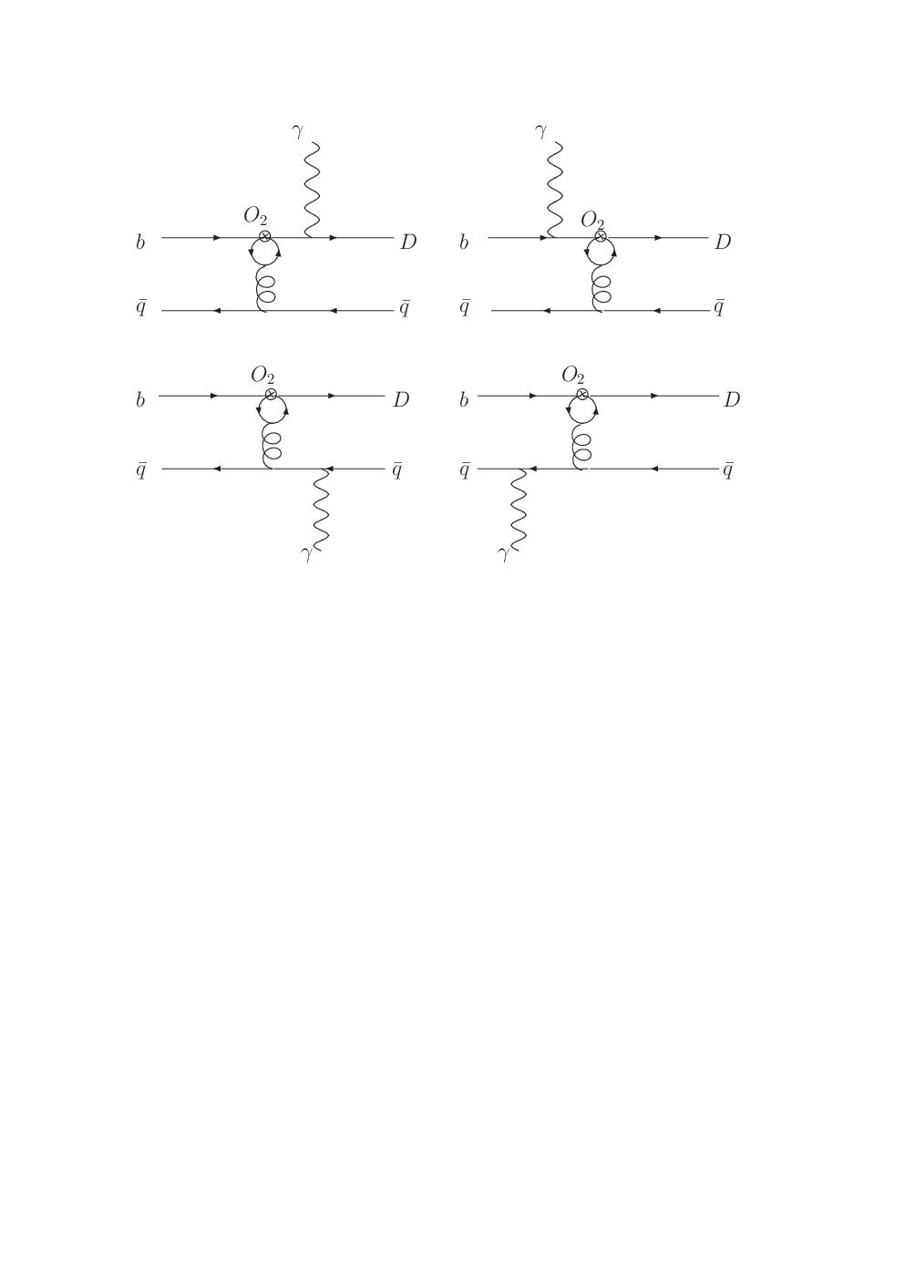
Figure 4: Feynman diagrams in which the operator O2O_{2} is inserted in the loop with a photon emitted from the external quark line

Next we want to mention some higher order corrections as usual which may give important contributions: charm and up quark loop (𝒪⁡(αs){\cal O}(\alpha_{s})) contributions in Fig. 4, Fig. 5 and Fig. 6. It should be pointed out that these contributions are not related to next-to-leading order corrections in pQCD approach, while next-to-leading order corrections to the exclusive processes π​γ∗→γ\pi\gamma^{*}\to\gamma in pQCD approach have been investigated in Ref. Nandi:2007qx.

We use the subtitle “quark line photon emission” to denote that a photon is emitted through the external quark lines as in Fig.4. We define the c{c} and u{u} loop function in order that the b→D​g{b\to Dg} vertex can be expressed as D¯​γμ​(1−γ5)​Iμ​νa​Aa​ν​b{\bar{D}\gamma^{\mu}(1-\gamma^{5})I^{a}_{\mu\nu}A^{a\nu}b}. It has the gauge invariant form Bander:1979px as follows:

Iμ​νa\displaystyle I_{\mu\nu}^{a} =\displaystyle= g​Ta2​π2​(k2​gμ​ν−kμ​kν)​∫01d​x​x​(1−x)​[1+log⁡(mi2−x⁡(1−x)​k2t2)]\displaystyle\frac{gT^{a}}{2\pi^{2}}(k^{2}g_{\mu\nu}-k_{\mu}k_{\nu})\int^{1}_{0}dxx(1-x)\left[1+\log\left(\frac{m_{i}^{2}-x(1-x)k^{2}}{t^{2}}\right)\right] (66)
=\displaystyle= −g​Ta8​π2​(k2​gμ​ν−kμ​kν)​[G⁡(mi2,k2,t)−23],\displaystyle-\frac{gT^{a}}{8\pi^{2}}(k^{2}g_{\mu\nu}-k_{\mu}k_{\nu})\left[G(m_{i}^{2},k^{2},t)-\frac{2}{3}\right],

where k{k} is the gluon momentum and mi{m_{i}} is the loop internal quark mass. G is the function from the loop integration:

G⁡(mi2,k2,t)\displaystyle G(m_{i}^{2},k^{2},t) =\displaystyle= θ⁡(−k2)​23​[53+4​mi2k2−ln⁡mi2t2+(1+2​mi2k2)​1−4​mi2k2​ln⁡1−4​mi2/k2−11−4​mi2/k2+1]\displaystyle\theta(-k^{2})\frac{2}{3}\left[\frac{5}{3}+\frac{4m_{i}^{2}}{k^{2}}-\ln{\frac{m_{i}^{2}}{t^{2}}}+\left(1+\frac{2m_{i}^{2}}{k^{2}}\right)\sqrt{1-\frac{4m_{i}^{2}}{k^{2}}}\ln{\frac{\sqrt{1-4m_{i}^{2}/k^{2}}-1}{\sqrt{1-4m_{i}^{2}/k^{2}}+1}}\right] (67)
+θ(k2)θ(4mi2−k2)23[53+4​mi2k2−lnmi2t2\displaystyle+\theta(k^{2})\theta(4m_{i}^{2}-k^{2})\frac{2}{3}\Bigg[\frac{5}{3}+\frac{4m_{i}^{2}}{k^{2}}-\ln{\frac{m_{i}^{2}}{t^{2}}}
−2(1+2​mi2k2)4​mi2k2−1arctan(14​mi2/k2−1)]\displaystyle-2\left(1+\frac{2m_{i}^{2}}{k^{2}}\right)\sqrt{\frac{4m_{i}^{2}}{k^{2}}-1}\arctan{\left(\frac{1}{\sqrt{4m_{i}^{2}/k^{2}-1}}\right)}\Bigg]
+θ(k2−4mi2)23[53+4​mi2k2−lnmi2t2\displaystyle+\theta(k^{2}-4m_{i}^{2})\frac{2}{3}\Bigg[\frac{5}{3}+\frac{4m_{i}^{2}}{k^{2}}-\ln{\frac{m_{i}^{2}}{t^{2}}}
+(1+2​mi2k2)1−4​mi2k2(ln1−1−4​mi2/k21+1−4​mi2/k2+iπ)].\displaystyle+\left(1+\frac{2m_{i}^{2}}{k^{2}}\right)\sqrt{1-\frac{4m_{i}^{2}}{k^{2}}}\left(\ln{\frac{1-\sqrt{1-4m_{i}^{2}/k^{2}}}{1+\sqrt{1-4m_{i}^{2}/k^{2}}}}+i\pi\right)\Bigg].

The loop function G{G} has the dependence of gluon momentum square of k2{k^{2}}. But there is no singularity when we take the limit of k→0{k\rightarrow 0}, so we can neglect kT{k_{T}} components of k2{k^{2}} in the loop function G{G}. Using this effective vertex, the factorization formulae for the first two diagrams of Fig.4 is calculated as:

M1​iL⁡(a)\displaystyle M^{L(a)}_{1i} =\displaystyle= −QDF∫01dx1dx2∫b1db1b2db2ϕB(x1,b1)C2(tb)Ee(tb)[G(mi2,−x1x2mB2,tb)−23]\displaystyle-Q_{D}F\int^{1}_{0}dx_{1}dx_{2}\int b_{1}db_{1}b_{2}db_{2}\phi_{B}(x_{1},b_{1})C_{2}(t_{b})E_{e}(t_{b})\Big[G(m_{i}^{2},-x_{1}x_{2}m_{B}^{2},t_{b})-\frac{2}{3}\Big] (68)
×[x22​rV​(ϕVv​(x2)+ϕVa​(x2))+3​x1​x2​ϕVT​(x2)]​he​(x1​x2,x2−1,b1,b2),\displaystyle\times\Big[x_{2}^{2}r_{V}(\phi_{V}^{v}(x_{2})+\phi_{V}^{a}(x_{2}))+3x_{1}x_{2}\phi_{V}^{T}(x_{2})\Big]h_{e}(x_{1}x_{2},x_{2}-1,b_{1},b_{2}),
M1​iR⁡(a)\displaystyle M^{R(a)}_{1i} =\displaystyle= −QbF∫01dx1dx2∫b1db1b2db2ϕB(x1,b1)C2(tb′)Ee′(tb′)[G(mi2,−x1x2mB2,tb′)−23]\displaystyle-Q_{b}F\int^{1}_{0}dx_{1}dx_{2}\int b_{1}db_{1}b_{2}db_{2}\phi_{B}(x_{1},b_{1})C_{2}(t_{b}^{\prime})E_{e}^{\prime}(t_{b}^{\prime})\Big[G(m_{i}^{2},-x_{1}x_{2}m_{B}^{2},t_{b}^{\prime})-\frac{2}{3}\Big] (69)
×x1​x2​rV​(ϕVa​(x2)−ϕVv​(x2))​he​(x1​x2,1+x1,b2,b1),\displaystyle\times x_{1}x_{2}r_{V}(\phi_{V}^{a}(x_{2})-\phi_{V}^{v}(x_{2}))h_{e}(x_{1}x_{2},1+x_{1},b_{2},b_{1}),

where QD=−13Q_{D}=-\frac{1}{3}. For the other two diagrams of Fig.4, the factorization formulas are

ℳ1​iL⁡(b)​(Qq)\displaystyle{\cal M}_{1i}^{L(b)}(Q_{q}) =\displaystyle= QqF∫01dx1dx2∫0∞b1db1b2db2ϕB(x1,b1){C2(tc)Ee(tc)\displaystyle Q_{q}F\int_{0}^{1}dx_{1}dx_{2}\int_{0}^{\infty}b_{1}db_{1}b_{2}db_{2}\phi_{B}(x_{1},b_{1})\bigg\{C_{2}(t_{c})E_{e}(t_{c}) (70)
×[x2​rV​(1+2​x2)​[ϕVv​(x2)+ϕVa​(x2)]+3​(x2−x1)​ϕVT​(x2)]\displaystyle\;\;\;\times\Big[x_{2}r_{V}(1+2x_{2})[\phi_{V}^{v}(x_{2})+\phi_{V}^{a}(x_{2})]+3(x_{2}-x_{1})\phi_{V}^{T}(x_{2})\Big]
×[G⁡(mi2,−(x1−x2)​mB2,tc)−23]​he​(x1−x2,−x2,b1,b2)\displaystyle\;\;\;\times\Big[G(m_{i}^{2},-(x_{1}-x_{2})m_{B}^{2},t_{c})-\frac{2}{3}\Big]h_{e}(x_{1}-x_{2},-x_{2},b_{1},b_{2})
+[x2​rV​(ϕVv​(x2)+ϕVa​(x2))−x1​ϕVT​(x2)]​[G⁡(mi2,−(x1−x2)​mB2,tc′)−23]\displaystyle+\Big[x_{2}r_{V}(\phi_{V}^{v}(x_{2})+\phi_{V}^{a}(x_{2}))-x_{1}\phi_{V}^{T}(x_{2})\Big]\Big[G(m_{i}^{2},-(x_{1}-x_{2})m_{B}^{2},t_{c}^{\prime})-\frac{2}{3}\Big]
×C2(tc′)Ee′(tc′)he(x1−x2,x1,b2,b1)},\displaystyle\;\;\;\times C_{2}(t_{c}^{\prime})E_{e}^{\prime}(t_{c}^{\prime})h_{e}(x_{1}-x_{2},x_{1},b_{2},b_{1})\bigg\},
ℳ1​iR⁡(b)​(Qq)\displaystyle{\cal M}_{1i}^{R(b)}(Q_{q}) =\displaystyle= Qq​F​∫01d​x1​d​x2​∫0∞b1​d​b1​b2​d​b2​ϕB​(x1,b1)​C2​(tc)​Ee​(tc)​he​(x1−x2,−x2,b1,b2)\displaystyle Q_{q}F\int_{0}^{1}dx_{1}dx_{2}\int_{0}^{\infty}b_{1}db_{1}b_{2}db_{2}\phi_{B}(x_{1},b_{1})C_{2}(t_{c})E_{e}(t_{c})h_{e}(x_{1}-x_{2},-x_{2},b_{1},b_{2}) (71)
×[G⁡(mi2,−(x1−x2)​mB2,tc)−23]×(2+x2)​x2​rV​[ϕVv​(x2)−ϕVa​(x2)].\displaystyle\;\;\;\times\Big[G(m_{i}^{2},-(x_{1}-x_{2})m_{B}^{2},t_{c})-\frac{2}{3}\Big]\times(2+x_{2})x_{2}r_{V}\Big[\phi_{V}^{v}(x_{2})-\phi_{V}^{a}(x_{2})\Big].
Refer to caption
Figure 5: Feynman diagrams in which the operator O2O_{2} is inserted in the loop with both of the photon and the virtual gluon emitted from the internal quark line.

In Fig. 5, we give the diagrams in which a photon emitted from the internal loop quark line. The sum of the effective vertex b→D​γ​g∗b\to D\gamma g^{*} in Fig.5 has been derived by Liu:1990yb; Simma:1990nr:

I=D¯​γρ​(1−γ5)​Ta​b​Iμ​ν​ρ​Aμ​Aa​ν,I=\bar{D}\gamma^{\rho}(1-\gamma_{5})T^{a}bI_{\mu\nu\rho}A^{\mu}A^{a\nu}, (72)

with the tensor structure given by

Iμ​ν​ρ\displaystyle I_{\mu\nu\rho} =\displaystyle= A4​[(q⋅k)​ϵμ​ν​ρ​σ​(q−k)σ+ϵν​ρ​σ​τ​qσ​kτ​kμ−ϵμ​ρ​σ​τ​qσ​kτ​qν]\displaystyle A_{4}\left[(q\cdot k)\epsilon_{\mu\nu\rho\sigma}(q-k)^{\sigma}+\epsilon_{\nu\rho\sigma\tau}q^{\sigma}k^{\tau}k_{\mu}-\epsilon_{\mu\rho\sigma\tau}q^{\sigma}k^{\tau}q_{\nu}\right] (73)
+A5​[ϵμ​ρ​σ​τ​qσ​kτ​kν−k2​ϵμ​ν​ρ​σ​qσ],\displaystyle\hskip-8.53581pt+A_{5}\left[\epsilon_{\mu\rho\sigma\tau}q^{\sigma}k^{\tau}k_{\nu}-k^{2}\epsilon_{\mu\nu\rho\sigma}q^{\sigma}\right],

and

A4\displaystyle A_{4} =\displaystyle= 4​i​e​g3​π2​∫01d​x​∫01−xd​y​x​yx⁡(1−x)​k2+2​x​y​q⋅k−mi2+i​ε,\displaystyle\frac{4ieg}{3\pi^{2}}\int_{0}^{1}dx\int_{0}^{1-x}dy\frac{xy}{x(1-x)k^{2}+2xyq\cdot k-m_{i}^{2}+i\varepsilon}, (74)
A5\displaystyle A_{5} =\displaystyle= −4​i​e​g3​π2∫01dx∫01−xdyx⁡(1−x)x⁡(1−x)​k2+2​x​y​q⋅k−mi2+i​ε,\displaystyle-\frac{4ieg}{3\pi^{2}}\int_{0}^{1}dx\int_{0}^{1-x}dy\frac{x(1-x)}{x(1-x)k^{2}+2xyq\cdot k-m_{i}^{2}+i\varepsilon}, (75)

where qq is the momentum of the photon q=PB−PVq=P_{B}-P_{V}, and kk is the momentum of the gluon. Then the amplitudes can be expressed as follows:

ℳ2​iL\displaystyle{\cal M}_{2i}^{L} =\displaystyle= −83F∫01dx∫01−xdy∫01dx1dx2∫b1db1ϕB(x1,b1)C2(td)αs(td)exp[−SB(td)]\displaystyle-\frac{8}{3}F\int^{1}_{0}dx\int^{1-x}_{0}dy\int^{1}_{0}dx_{1}dx_{2}\int b_{1}db_{1}\phi_{B}(x_{1},b_{1})C_{2}(t_{d})\alpha_{s}(t_{d})\exp[-S_{B}(t_{d})] (76)
×he′x​y​x2​mB2−mi2×{xyx2[(1−x2)rV(ϕVv(x2)+ϕVa(x2))−(1+2x1)ϕVT(x2)]\displaystyle\times\frac{h_{e}^{\prime}}{xyx_{2}m_{B}^{2}-m_{i}^{2}}\times\bigg\{xyx_{2}\Big[(1-x_{2})r_{V}(\phi_{V}^{v}(x_{2})+\phi_{V}^{a}(x_{2}))-(1+2x_{1})\phi_{V}^{T}(x_{2})\Big]
+x(1−x)[x22rV(ϕVv(x2)+ϕVa(x2))+3x1x2ϕVT(x2)]},\displaystyle\;\;+x(1-x)\Big[x_{2}^{2}r_{V}(\phi_{V}^{v}(x_{2})+\phi_{V}^{a}(x_{2}))+3x_{1}x_{2}\phi_{V}^{T}(x_{2})\Big]\bigg\},
ℳ2​iR\displaystyle{\cal M}_{2i}^{R} =\displaystyle= 83​F​∫01d​x​∫01−xd​y​∫01d​x1​d​x2​∫b1​d​b1​ϕB​(x1,b1)​C2​(td)​αs​(td)​exp⁡[−SB​(td)]\displaystyle\frac{8}{3}F\int^{1}_{0}dx\int^{1-x}_{0}dy\int^{1}_{0}dx_{1}dx_{2}\int b_{1}db_{1}\phi_{B}(x_{1},b_{1})C_{2}(t_{d})\alpha_{s}(t_{d})\exp[-S_{B}(t_{d})] (77)
×he′x​y​x2​mB2−mi2×x​y​x22​rV​[ϕVv​(x2)−ϕVa​(x2)],\displaystyle\times\frac{h_{e}^{\prime}}{xyx_{2}m_{B}^{2}-m_{i}^{2}}\times xyx_{2}^{2}r_{V}\Big[\phi_{V}^{v}(x_{2})-\phi_{V}^{a}(x_{2})\Big],

where the function he′h_{e}^{\prime} is defined by:

he′\displaystyle h_{e}^{\prime} ≡\displaystyle\equiv K0​(x1​x2​mB​b1)−[θ⁡(B2)​K0​(b1​|B2|)+θ⁡(−B2)​i​π2​H0​(b1​|B2|)],\displaystyle K_{0}(\sqrt{x_{1}x_{2}}m_{B}b_{1})-\Big[\theta(B^{2})K_{0}(b_{1}\sqrt{|B^{2}|})+\theta(-B^{2})i\frac{\pi}{2}H_{0}(b_{1}\sqrt{|B^{2}|})\Big], (78)

with

B2\displaystyle B^{2} =\displaystyle= x1​x2​mB2−y1−x​x2​mB2+mi2x⁡(1−x).\displaystyle x_{1}x_{2}m_{B}^{2}-\frac{y}{1-x}x_{2}m_{B}^{2}+\frac{m_{i}^{2}}{x(1-x)}. (79)
Refer to caption
Figure 6: Feynman diagrams in which the operator O2O_{2} is inserted in the loop with a photon emitted from the internal quark line

Diagrams in Fig. 6 in which the photon is emitted from the external loop and the gluon is emitted from QCD interaction Hamiltonian do not give any contribution to B→V​γB\to V\gamma. The reason is as follows. Similar with b→D​gb\to Dg, the vertex for b→D​γb\to D\gamma can also be expressed as D¯​γμ​Aν​(1−γ5)​(k2​gμ​ν−kμ​kν)​b{\bar{D}\gamma^{\mu}A^{\nu}(1-\gamma^{5})(k^{2}g_{\mu\nu}-k_{\mu}k_{\nu})b} only with a different coefficient. For an on-shell photon, the following conditions are required: k2=0k^{2}=0 and ϵ⋅k=0\epsilon\cdot k=0, thus the contribution from diagrams in Fig. 6 vanishes in b→s⁡(d)​γb\to s(d)\gamma decays. But it should be noted that these diagrams can give a non-zero contribution to b→s⁡(d)​γ∗→s⁡(d)​l+​l−b\to s(d)\gamma^{*}\to s(d)l^{+}l^{-}.

Refer to caption
Figure 7: Feynman diagrams for annihilation topologies

In annihilation diagrams, there are three different kinds of operators in the ⊗\otimes depicted in Fig. 7. In the following, we use L​LLL to denote the left-handed current between bb and q¯\bar{q} quark and the left-handed current between the final state two quarks; L​RLR denotes the left-handed current between bb and q¯\bar{q} quark and the right-handed current between the final state two quarks; we use S​PSP to denote the (S−P)​(S+P)(S-P)(S+P) current which is from the Fierz transformation of (V−A)​(V+A)(V-A)(V+A) operators. The factorization formulae for these diagrams are given by:

ℳa​n​nL⁡(a,L​L)​(ai,Qq1)\displaystyle{\cal M}_{ann}^{L(a,LL)}(a_{i},Q_{q_{1}}) =\displaystyle= ℳa​n​nL⁡(a,L​R)​(ai,Qq1)\displaystyle{\cal M}_{ann}^{L(a,LR)}(a_{i},Q_{q_{1}}) (80)
=\displaystyle= F​3​6​Qq1​rV​fV​π2​mB2​∫01d​x1​∫0∞b1​d​b1​ai​(te′)​Ea​(te′)​ϕB​(x1,b1)​K0​(x1​mB​b1),\displaystyle F\frac{3\sqrt{6}Q_{q_{1}}r_{V}f_{V}\pi}{2m_{B}^{2}}\int^{1}_{0}dx_{1}\int_{0}^{\infty}b_{1}db_{1}a_{i}(t_{e}^{\prime})E_{a}(t_{e}^{\prime})\phi_{B}(x_{1},b_{1})K_{0}(\sqrt{x}_{1}m_{B}b_{1}),
ℳa​n​nR⁡(a,L​L)​(ai,Qq1)\displaystyle{\cal M}_{ann}^{R(a,LL)}(a_{i},Q_{q_{1}}) =\displaystyle= ℳa​n​nR⁡(a,L​R)​(ai,Qq1)\displaystyle{\cal M}_{ann}^{R(a,LR)}(a_{i},Q_{q_{1}}) (81)
=\displaystyle= −F3​6​Qb​rV​fV​π2​mB2∫01dx1∫0∞b1db1ai(te)Ea(te)ϕB(x1,b1)K0(1+x1mBb1),\displaystyle-F\frac{3\sqrt{6}Q_{b}r_{V}f_{V}\pi}{2m_{B}^{2}}\int^{1}_{0}dx_{1}\int_{0}^{\infty}b_{1}db_{1}a_{i}(t_{e})E_{a}(t_{e})\phi_{B}(x_{1},b_{1})K_{0}(\sqrt{1+x_{1}}m_{B}b_{1}),
ℳa​n​nL⁡(b,L​L)​(ai,Qq2,Qq3)\displaystyle{\cal M}_{ann}^{L(b,LL)}(a_{i},Q_{q_{2}},Q_{q_{3}}) =\displaystyle= ℳa​n​nR⁡(b,L​R)​(ai,Qq2,Qq3)\displaystyle{\cal M}_{ann}^{R(b,LR)}(a_{i},Q_{q_{2}},Q_{q_{3}}) (82)
=\displaystyle= −F3​6​rV​fB​π2​mB2∫01dx2∫b2db2[ϕVv(x2)+ϕVa(x2)]\displaystyle-F\frac{3\sqrt{6}r_{V}f_{B}\pi}{2m_{B}^{2}}\int^{1}_{0}dx_{2}\int b_{2}db_{2}\Big[\phi_{V}^{v}(x_{2})+\phi_{V}^{a}(x_{2})\Big]
×\displaystyle\times {Qq2ai(tf)Ea′(tf)iπ2H0(1)(1−x2mBb2)\displaystyle\bigg\{Q_{q_{2}}a_{i}(t_{f})E^{\prime}_{a}(t_{f})i\frac{\pi}{2}H_{0}^{(1)}(\sqrt{1-x_{2}}m_{B}b_{2})
−x2Qq3ai(tf′)Ea′(tf′)iπ2H0(1)(x2mBb2)},\displaystyle-x_{2}Q_{q_{3}}a_{i}(t_{f}^{\prime})E^{\prime}_{a}(t_{f}^{\prime})i\frac{\pi}{2}H_{0}^{(1)}(\sqrt{x_{2}}m_{B}b_{2})\bigg\},
ℳa​n​nR⁡(b,L​L)​(ai,Qq2,Qq3)\displaystyle{\cal M}_{ann}^{R(b,LL)}(a_{i},Q_{q_{2}},Q_{q_{3}}) =\displaystyle= ℳa​n​nL⁡(b,L​R)​(ai,Qq2,Qq3)\displaystyle{\cal M}_{ann}^{L(b,LR)}(a_{i},Q_{q_{2}},Q_{q_{3}}) (83)
=\displaystyle= −F3​6​rV​fB​π2​mB2∫10dx2∫b2db2\displaystyle-F\frac{3\sqrt{6}r_{V}f_{B}\pi}{2m_{B}^{2}}\int^{1}_{0}dx_{2}\int b_{2}db_{2}
×\displaystyle\times {(1−x2)[ϕVv(x2)−ϕVa(x2)]Qq2ai(tf)Ea′(tf)iπ2H0(1)(1−x2mBb2)\displaystyle\bigg\{(1-x_{2})\Big[\phi_{V}^{v}(x_{2})-\phi_{V}^{a}(x_{2})\Big]Q_{q_{2}}a_{i}(t_{f})E^{\prime}_{a}(t_{f})i\frac{\pi}{2}H_{0}^{(1)}(\sqrt{1-x_{2}}m_{B}b_{2})
−[ϕVv(x2)−ϕVa(x2)]Qq3ai(tf′)Ea′(tf′)iπ2H0(1)(x2mBb2)},\displaystyle\;\;\;-\Big[\phi_{V}^{v}(x_{2})-\phi_{V}^{a}(x_{2})\Big]Q_{q_{3}}a_{i}(t_{f}^{\prime})E^{\prime}_{a}(t_{f}^{\prime})i\frac{\pi}{2}H_{0}^{(1)}(\sqrt{x_{2}}m_{B}b_{2})\bigg\},
ℳa​n​nL⁡(S​P)​(ai)\displaystyle{\cal M}_{ann}^{L(SP)}(a_{i}) =\displaystyle= F​3​6​fB​πmB2​∫01d​x2​∫b2​d​b2​ϕVT​(x2)\displaystyle F\frac{3\sqrt{6}f_{B}\pi}{m_{B}^{2}}\int^{1}_{0}dx_{2}\int b_{2}db_{2}\phi_{V}^{T}(x_{2}) (84)
×\displaystyle\times {Qq2​ai​(tf)​Ea′​(tf)​i​π2​H0(1)​(1−x2​mB​b2)+Qq3​ai​(tf′)​Ea′​(tf′)​i​π2​H0(1)​(x2​mB​b2)}.\displaystyle\bigg\{Q_{q_{2}}a_{i}(t_{f})E^{\prime}_{a}(t_{f})i\frac{\pi}{2}H_{0}^{(1)}(\sqrt{1-x_{2}}m_{B}b_{2})+Q_{q_{3}}a_{i}(t_{f}^{\prime})E^{\prime}_{a}(t_{f}^{\prime})i\frac{\pi}{2}H_{0}^{(1)}(\sqrt{x_{2}}m_{B}b_{2})\bigg\}.
Refer to caption
Figure 8: Feynman diagrams with double-photon contributions

Finally, there is another kind of contribution from O7​γO_{7\gamma}: the neutral vector meson q¯​q\bar{q}q is generated by a photon as depicted in Fig. 8. Although these diagrams are suppressed by the electromagnetic coupling constant, the enhancement factor mB/ΛQ​C​Dm_{B}/\Lambda_{QCD} can make it important in some cases Lu:2006nz. We include these diagrams in our calculation. The first two diagrams of Fig. 8 are equal to each other, so are the last two diagrams. The factorization formulae are given by:

ℳe​nL​(Qq)\displaystyle{\cal M}_{en}^{L}(Q_{q}) =\displaystyle= −F3​6​αe​m​Qq​Qb​rb​fVmB​mV∫01dx1∫0∞b1db1ϕB(x1,b1)\displaystyle-F\frac{3\sqrt{6}\alpha_{em}Q_{q}Q_{b}r_{b}f_{V}}{m_{B}m_{V}}\int^{1}_{0}dx_{1}\int_{0}^{\infty}b_{1}db_{1}\phi_{B}(x_{1},b_{1}) (85)
×{C7​γ​(te)​Ea​(te)​K0​(1+x1​mB​b1)+C7​γ​(te′)​Ea​(te′)​K0​(x1​mB​b1)},\displaystyle\times\bigg\{C_{7\gamma}(t_{e})E_{a}(t_{e})K_{0}(\sqrt{1+x_{1}}m_{B}b_{1})+C_{7\gamma}(t_{e}^{\prime})E_{a}(t_{e}^{\prime})K_{0}(\sqrt{x_{1}}m_{B}b_{1})\bigg\},
ℳe​nR​(Qq)\displaystyle{\cal M}_{en}^{R}(Q_{q}) =\displaystyle= −rDrb​ℳe​nL​(Qq).\displaystyle-\frac{r_{D}}{r_{b}}{\cal M}_{en}^{L}(Q_{q}). (86)

IV.2 Numerical results of Branching ratios

With those decay amplitude formulas for different Feynman diagrams in the last subsection, it is easy to get the total decay amplitude for each channel of B→V​γB\to V\gamma: B−→ρ−​γB^{-}\to\rho^{-}\gamma, B0→ρ0​γB^{0}\to\rho^{0}\gamma, B0→ω​γB^{0}\to\omega\gamma, B−→K∗⁣−​γB^{-}\to K^{*-}\gamma, B0→ϕ​γB^{0}\to\phi\gamma, B0→K∗0​γB^{0}\to K^{*0}\gamma, Bs0→K∗0​γB_{s}^{0}\to K^{*0}\gamma, Bs0→ρ0​γB_{s}^{0}\to\rho^{0}\gamma, Bs0→ω​γB_{s}^{0}\to\omega\gamma, and Bs0→ϕ​γB_{s}^{0}\to\phi\gamma. The explicit expressions are shown in Appendix B. The CP-averaged decay width is then

Γ⁡(B→V​γ)=|𝒜⁡(B¯→V​γ)|2+|𝒜⁡(B→V¯​γ)|232​π​mB​(1−rV2)3,\displaystyle\Gamma(B\to V\gamma)=\frac{|{\cal A}(\bar{B}\to V\gamma)|^{2}+|{\cal A}(B\to\bar{V}\gamma)|^{2}}{32\pi m_{B}}(1-r_{V}^{2})^{3}, (87)

where the summation on polarizations is implemented.

For CKM matrix elements, we use the same values as in Ref. Ali:2007ff:

|Vu​d|=0.974,|Vu​s|=0.226,|Vu​b|=(3.68−0.08+0.11)×10−3,|Vt​d|=(8.20−0.27+0.59)×10−3,|Vt​s|=40.96×10⁻³,|Vt​b|=1.0,α=(99−9.4+4)∘,γ=(59.0−3.7+9.7)∘,arg​[−Vt​s​Vt​b∗]=1.0∘,\begin{array}[]{lll}|V_{ud}|=0.974,&|V_{us}|=0.226,&|V_{ub}|=(3.68^{+0.11}_{-0.08})\times 10^{-3},\\ |V_{td}|=(8.20^{+0.59}_{-0.27})\times 10^{-3},&|V_{ts}|=40.96\times 10^{-3},&|V_{tb}|=1.0,\\ \alpha={(99^{+4}_{-9.4})}^{\circ},&\gamma=(59.0^{+9.7}_{-3.7})^{\circ},&\mbox{arg}[-V_{ts}V^{*}_{tb}]={1.0}^{\circ},\end{array} (88)

where we have adopted the updated results from Charles:2004jd and drop the (small) errors on Vu​dV_{ud}, Vu​sV_{us}, Vt​sV_{ts} and Vt​bV_{tb}. The CKM factors mostly give an overall factor to branching ratios. However, the CKM angles do give large uncertainties to branching ratios of some decay modes and to all the non-zero CP asymmetries which will be discussed in the following subsection.

Table 7: C​PCP-averaged branching ratios (×10−6\times 10^{-6}) of B→V​γB\to V\gamma decays obtained in pQCD approach (This work); the errors for these entries correspond to uncertainties in input hadronic quantities, from the scale-dependence, and CKM matrix elements, respectively. For comparison, we also listed the current experimental measurements Barberio:2006bi; Drutskoy:2007aj; Aubert:2006pu; Abe:2005rj and theoretical estimates of branching ratios recently given in Ref. Ball:2006eu (QCDF) and in Ref. Ali:2007sj (SCET).
Modes QCDF SCET This work Exp.
B−→K∗⁣−​γB^{-}\to K^{*-}\gamma 53.3±13.5±5.853.3\pm 13.5\pm 5.8 46±12±4±2±146\pm 12\pm 4\pm 2\pm 1 35.8−12.8−4.0−1.1+17.6+5.4+1.135.8_{-12.8-4.0-1.1}^{+17.6+5.4+1.1} 40.3±2.640.3\pm 2.6  [HFAG]
B¯0→K¯∗0​γ\bar{B}^{0}\to\bar{K}^{*0}\gamma 54.2±13.2±6.754.2\pm 13.2\pm 6.7 43±11±4±2±143\pm 11\pm 4\pm 2\pm 1 38.1−12.7−3.8−1.1+17.3+5.5+1.138.1^{+17.3+5.5+1.1}_{-12.7-3.8-1.1} 40.1±2.040.1\pm 2.0   [HFAG]
B¯s0→ϕ​γ\bar{B}_{s}^{0}\to\phi\gamma 39.4±10.7±5.339.4\pm 10.7\pm 5.3 43±11±3±3±143\pm 11\pm 3\pm 3\pm 1 35.8−10.3−3.5−1.1+13.7+4.9+1.135.8_{-10.3-3.5-1.1}^{+13.7+4.9+1.1} 57−15−11+18+1257^{+18+12}_{-15-11} [Belle]
Modes QCDF This work Exp.
B−→ρ−​γB^{-}\to\rho^{-}\gamma 1.16±0.22±0.131.16\pm 0.22\pm 0.13 1.15−0.39−0.11−0.09+0.57+0.18+0.171.15^{+0.57+0.18+0.17}_{-0.39-0.11-0.09} 1.10−0.33+0.37±0.091.10^{+0.37}_{-0.33}\pm 0.09 [BaBar] 0.55−0.36−0.08+0.42+0.090.55^{+0.42+0.09}_{-0.36-0.08} [Belle]
B¯0→ρ0​γ\bar{B}^{0}\to\rho^{0}\gamma 0.55±0.11±0.070.55\pm 0.11\pm 0.07 0.57−0.19−0.06−0.04+0.26+0.09+0.080.57^{+0.26+0.09+0.08}_{-0.19-0.06-0.04} 0.79−0.20+0.22±0.060.79^{+0.22}_{-0.20}\pm 0.06 [BaBar] 1.25−0.33−0.06+0.37+0.071.25^{+0.37+0.07}_{-0.33-0.06} [Belle]
B¯0→ω​γ\bar{B}^{0}\to\omega\gamma 0.44±0.09±0.050.44\pm 0.09\pm 0.05 0.51−0.17−0.05−0.03+0.23+0.08+0.080.51^{+0.23+0.08+0.08}_{-0.17-0.05-0.03} 0.40−0.20+0.24±0.050.40^{+0.24}_{-0.20}\pm 0.05 [BaBar] 0.56−0.27−0.10+0.34+0.050.56^{+0.34+0.05}_{-0.27-0.10} [Belle]
B¯s0→K∗0​γ\bar{B}_{s}^{0}\to K^{*0}\gamma 1.26±0.25±0.181.26\pm 0.25\pm 0.18 1.11−0.32−0.12−0.07+0.42+0.15+0.161.11_{-0.32-0.12-0.07}^{+0.42+0.15+0.16} —
B¯0→ϕ​γ\bar{B}^{0}\to\phi\gamma — (7.5−2.1−0.9−0.5+2.8+2.1+1.1)×10−6(7.5_{-2.1-0.9-0.5}^{+2.8+2.1+1.1})\times 10^{-6} <0.85<0.85  [HFAG]
B¯s0→ρ0​γ\bar{B}_{s}^{0}\to\rho^{0}\gamma — (1.7−0.4−0.1−0.1+0.4+0.1+0.0)×10−3(1.7_{-0.4-0.1-0.1}^{+0.4+0.1+0.0})\times 10^{-3} —
B¯s0→ω​γ\bar{B}_{s}^{0}\to\omega\gamma — (1.8−0.4−0.2−0.1+0.4+0.1+0.1)×10−4(1.8_{-0.4-0.2-0.1}^{+0.4+0.1+0.1})\times 10^{-4} —

C​PCP-averaged branching ratios of B→V​γB\to V\gamma decays are listed in table 7. The first error in these entries arises from the input hadronic parameters, which is dominated by B⁡(Bs)B(B_{s})-meson decay constants (taken as fB=(0.19±0.02)f_{B}=(0.19\pm 0.02) GeV and fBs=(0.23±0.02)f_{B_{s}}=(0.23\pm 0.02) GeV) and BB (BsB_{s}) meson wave function shape parameters (taken as ωB=(0.40±0.05)\omega_{B}=(0.40\pm 0.05) GeV and ωBs=(0.50±0.05)\omega_{B_{s}}=(0.50\pm 0.05) GeV). The second error is from the hard scale tt, defined in Eqs. (A1) – (A8) in Appendix A, which we vary from 0.75​t0.75t to 1.25​t1.25t (not changing 1/bi1/b_{i}), and from ΛQ​C​D(5)=0.25±0.05\Lambda^{(5)}_{QCD}=0.25\pm 0.05 GeV. This scale-dependence characterize the size of next-to-leading order contributions in pQCD approach. A part of this perturbative improvement coming from next-to-leading order Wilson coefficients is already available Buchalla:1995vs. However, the complete next-to-leading order corrections to hard spectator kernels are still missing. The third error is the combined uncertainties in CKM matrix elements and angles of the unitarity triangle. It is clear that the largest uncertainty here is the first one from the input hadronic parameters.

These ten B→V​γB\to V\gamma decay channels can be divided into three different types: b→sb\to s transitions, b→db\to d transitions and purely annihilation decays. The first type contains B¯0→K¯∗0​γ\bar{B}^{0}\to\bar{K}^{*0}\gamma, B−→K∗⁣−​γB^{-}\to K^{*-}\gamma and B¯s→ϕ​γ\bar{B}_{s}\to\phi\gamma. Among these decays, the dominant contribution from O7​γO_{7\gamma}, is proportional to Vt​b​Vt​s∗∼λ2V_{tb}V_{ts}^{*}\sim\lambda^{2}. This contribution can be related to the form factor T1B→VT_{1}^{B\to V}. In the flavor SU(3) symmetry limit, form factors for these three channels should be equal which could also relates the three decays. We do obtain similar branching ratios for this kind decays only with small deviations. The penguin contribution in b→d​γb\to d\gamma processes is proportional to Vt​b​Vt​d∗∼λ3V_{tb}V_{td}^{*}\sim\lambda^{3}, which is expected to be suppressed by one order magnitude relative to the b→sb\to s transitions. In our calculation, branching ratio results for pure annihilation processes are mainly from two-photon diagrams in Fig. 8. Thus ℬℛ⁡(B→ϕ​γ){\cal BR}(B\to\phi\gamma) is surely consistent with Ref. Lu:2006nz. This feature can also certainly interpret the large differences between B¯s→ρ0​γ\bar{B}_{s}\to\rho^{0}\gamma and B¯s→ω​γ\bar{B}_{s}\to\omega\gamma. This contribution is proportional to the charge of the constitute quark. This factor is 23−−13\frac{2}{3}-\frac{-1}{3} for ρ0\rho^{0} while 23+−13\frac{2}{3}+\frac{-1}{3} for ω\omega. Thus the branching ratio of Bs→ρ0​γB_{s}\to\rho^{0}\gamma is one order in magnitude larger than that of (Bs→ω​γ)(B_{s}\to\omega\gamma).

In the literature, there are many studies concentrating on B→V​γB\to V\gamma Li:1998tk; Li:2003kz; Keum:2004is; Lu:2005yz; Li:2006xe; Ali:2001ez; Beneke:2004dp; Bosch:2001gv; Bosch:2002bw; Becher:2005fg; Chay:2003kb; Bosch:2004nd; Ali:2004hn; Ali:2006fa; Ali:2007sj. Recently, a comprehensive study Ball:2006eu using QCDF method and QCD sum rules appears. In that paper, the authors used QCDF approach to calculate all B→V​γB\to V\gamma approach and included some power corrections: weak annihilation contributions, the soft-gluon emission from quark (charm and light-quark) loops and long distance photon emission from the soft quarks. In Table 7, we quote them to make a comparison. Their uncertainties come from form factors, the renormalization scale, the soft-gluon terms, the CKM parameters, decay constants, Gegenbauer moments, the first inverse moments of BB(BsB_{s}) mesons and quark masses, etc. Their results for branching ratios of B−→K∗⁣−​γB^{-}\to K^{*-}\gamma and B¯0→K¯∗0​γ\bar{B}^{0}\to\bar{K}^{*0}\gamma are about (20CLOSE(20OPEN−50)%-50)\% larger than our predictions. The main reason is differences in form factors T1T_{1}: they used T1B→K∗=0.31±0.04T_{1}^{B\to K^{*}}=0.31\pm 0.04 while our calculation gives a smaller T1=0.23−0.04+0.05T_{1}=0.23^{+0.05}_{-0.04}. The smaller form factor is also preferred by recent Lattice QCD result: T1B→K∗=0.24±0.03−0.01+0.04T_{1}^{B\to K^{*}}=0.24\pm 0.03^{+0.04}_{-0.01}. Although the difference is not too large, it can already induce a sizable difference to branching ratios. b→db\to d transitions and B¯s→ϕ​γ\bar{B}_{s}\to\phi\gamma are well consistent with each other, as the effective form factors used in Ref. Ball:2006eu are smaller and almost equal to our results. Very recently, the authors in Ref. Ali:2007sj used the more theoretical approach SCET to investigate the three b→sb\to s decays channels: B−→K∗⁣−​γB^{-}\to K^{*-}\gamma, B¯0→K¯∗0​γ\bar{B}^{0}\to\bar{K}^{*0}\gamma and B¯s→ϕ​γ\bar{B}_{s}\to\phi\gamma. After integrating out the hard scale mbm_{b} which results in SCETI, contributions to B→V​γB\to V\gamma decay amplitudes can be divided into two different groups: contributions from operators JAJ_{A} and JBJ_{B}. The BB-type operator is power suppressed in SCETI but it can give leading power contributions when matching onto SCETII as AA-type operator receives power suppressions. When performing the matching from SCETI to SCETII, we have to be cautious about the AA-type operator as this term suffers from the end-point singularities. Thus one has to leave it as a non-perturbative free parameter determined from experiments or some non-perturbative QCD approaches, but recent studies using zero-bin subtractions show that this term can also factorized in rapidity space Manohar:2006nz. In Ref. Ali:2007sj, the authors calculated the two-loop corrections (αs2\alpha_{s}^{2}) to short-distance coefficients of the AA-type operator (called vertex functions) determined from QCD to SCETI matching and utilized the physical B→VB\to V form factor T1T_{1} to extract the soft form factor in SCET. While for the BB-type operator which can been factorized into convolutions of LCDAs and hard kernels, both of the Wilson coefficient and jet function have been calculated up to one loop order. Short-distance Wilson coefficients for the BB-type operator are extracted at the scale mbm_{b} and have been evolved down the intermediate scale μ∼1.5\mu\sim 1.5 GeV using renormalization group equations. With these results, the authors find: compared with the leading order contribution, the order αs\alpha_{s} corrections from vertex corrections and hard spectator scattering can be as large as 10%\% and both of them also provide imaginary amplitudes about 5%5\% in magnitude; the order αs2\alpha_{s}^{2} corrections are not too large. We quote their final results for branching ratios in table 7 and they are also consistent with ours.

The three experimental collaborations, BaBar Aubert:2004te, Belle Nakao:2004th and CLEO Coan:1999kh, have reported their measurements on ℬℛ⁡(B→K∗​γ){\cal BR}(B\to K^{*}\gamma). Since all of these results are well consistent with each other, we quote the averaging results from Heavy Flavor Averaging Group (HFAG) Barberio:2006bi in table 7. We also include the very recent result on ℬℛ⁡(B¯s0→ϕ​γ){\cal{BR}}(\bar{B}_{s}^{0}\to\phi\gamma) Drutskoy:2007aj. All of them agree with our calculations. On the b→db\to d transition, branching ratios of some channels have been given by the BaBar Aubert:2006pu and Belle Abe:2005rj collaboration. We find that our results agree well with BaBar’s results but not with Belle’s central value results. In flavor SU(3) symmetry limit, the relation ℬℛ⁡(B−→ρ−​γ)=2​ℬℛ​(B¯0→ρ0​γ)=ℬℛ⁡(B¯0→ω​γ){\cal BR}(B^{-}\to\rho^{-}\gamma)=2{\cal BR}(\bar{B}^{0}\to\rho^{0}\gamma)={\cal BR}(\bar{B}^{0}\to\omega\gamma) should be held. The small deviation in our calculation is caused by the SU(3) symmetry breaking effect. Since the electro-magnetic penguin operator O7​γO_{7\gamma} gives the dominant contribution, it is difficult to understand the results from Belle collaboration: why is the branching ratio of B¯0→ρ0​γ\bar{B}^{0}\to\rho^{0}\gamma larger than B−→ρ−​γB^{-}\to\rho^{-}\gamma. But before we conclude it is the signal for non-standard model scenarios, it is necessary to re-examine this channel on the experimental side. All other decay modes, including B¯s\bar{B}_{s} decays and annihilation type decays, have not been experimentally measured.

IV.3 CP asymmetry studies

The direct CP-asymmetry in B¯→V​γ\bar{B}\to V\gamma is defined by:

ACPd​i​r≡ℬℛ⁡(B¯→V¯​γ)−ℬℛ⁡(B→V​γ)ℬℛ⁡(B¯→V¯​γ)+ℬℛ⁡(B→V​γ)=|𝒜⁡(B¯→V¯​γ)|2−|𝒜⁡(B→V​γ)|2|𝒜⁡(B¯→V¯​γ)|2+|𝒜⁡(B→V​γ)|2.\displaystyle A^{dir}_{\mathrm{CP}}\equiv\frac{{\cal BR}(\bar{B}\to\bar{V}\gamma)-{\cal BR}(B\to V\gamma)}{{\cal BR}(\bar{B}\to\bar{V}\gamma)+{\cal BR}(B\to V\gamma)}=\frac{|{\cal A}(\bar{B}\to\bar{V}\gamma)|^{2}-|{\cal A}(B\to V\gamma)|^{2}}{|{\cal A}(\bar{B}\to\bar{V}\gamma)|^{2}+|{\cal A}(B\to V\gamma)|^{2}}. (89)

In order to give a non-zero direct CP asymmetry, we need two kinds of contributions with different strong phases and different weak phases. The magnitude of the CP asymmetry also depends on relative sizes of the two different amplitudes: if one amplitude is much larger than the other one, we can only get a small CP asymmetry. Since there is only penguin contribution in B¯0→ϕ​γ\bar{B}^{0}\to\phi\gamma process, the direct CP asymmetry is zero. In other B→V​γB\to V\gamma decays, there are contributions from the penguin operator and two kinds of tree operators (proportional to Vc​b​Vc​d,c​s∗V_{cb}V^{*}_{cd,cs} and Vu​b​Vu​d,u​s∗V_{ub}V^{*}_{ud,us}). Taking these amplitudes into account, we obtain the numerical results for direct CP asymmetries (in %\%) in other B→V​γB\to V\gamma decays as:

ACPd​i​r​(B−→ρ−​γ)\displaystyle A^{dir}_{\rm{CP}}(B^{-}\to\rho^{-}\gamma) =\displaystyle= 12.8−0.3−1.8−0.8+0.8+2.9+0.8,\displaystyle 12.8^{+0.8+2.9+0.8}_{-0.3-1.8-0.8}, (90)
ACPd​i​r​(B¯0→ρ0​γ)\displaystyle A^{dir}_{\mathrm{CP}}(\bar{B}^{0}\to\rho^{0}\gamma) =\displaystyle= 12.4−0.4−2.4−0.9+0.2+1.8+0.5,\displaystyle 12.4^{+0.2+1.8+0.5}_{-0.4-2.4-0.9}, (91)
ACPd​i​r​(B−→K∗⁣−​γ)\displaystyle A^{dir}_{\mathrm{CP}}(B^{-}\to K^{*-}\gamma) =\displaystyle= −0.4±0.0±0.1±0.0,\displaystyle-0.4\pm 0.0\pm 0.1\pm 0.0, (92)
ACPd​i​r​(B¯0→K¯∗0​γ)\displaystyle A^{dir}_{\mathrm{CP}}(\bar{B}^{0}\to\bar{K}^{*0}\gamma) =\displaystyle= −0.3−0.0−0.0−0.0+0.0+0.0+0.0,\displaystyle-0.3_{-0.0-0.0-0.0}^{+0.0+0.0+0.0}, (93)
ACPd​i​r​(B¯0→ω​γ)\displaystyle A^{dir}_{\mathrm{CP}}(\bar{B}^{0}\to\omega\gamma) =\displaystyle= 12.1−0.2−2.4−0.8+0.0+1.8+0.5,\displaystyle 12.1^{+0.0+1.8+0.5}_{-0.2-2.4-0.8}, (94)
ACPd​i​r​(B¯s0→ρ0​γ)\displaystyle A^{dir}_{\mathrm{CP}}(\bar{B}^{0}_{s}\to\rho^{0}\gamma) =\displaystyle= −0.1−0.0−0.1−0.0+0.0+0.3+0.0,\displaystyle-0.1_{-0.0-0.1-0.0}^{+0.0+0.3+0.0}, (95)
ACPd​i​r​(B¯s0→K∗0​γ)\displaystyle A^{dir}_{\mathrm{CP}}(\bar{B}^{0}_{s}\to K^{*0}\gamma) =\displaystyle= 12.7−0.5−2.3−0.9+0.1+1.6+0.5,\displaystyle 12.7_{-0.5-2.3-0.9}^{+0.1+1.6+0.5}, (96)
ACPd​i​r​(B¯s0→ω​γ)\displaystyle A^{dir}_{\mathrm{CP}}(\bar{B}^{0}_{s}\to\omega\gamma) =\displaystyle= −0.3−0.0−0.5−0.0+0.0+0.9+0.0,\displaystyle-0.3_{-0.0-0.5-0.0}^{+0.0+0.9+0.0}, (97)
ACPd​i​r​(B¯s0→ϕ​γ)\displaystyle A^{dir}_{\mathrm{CP}}(\bar{B}^{0}_{s}\to\phi\gamma) =\displaystyle= −0.3−0.0−0.0−0.0+0.0+0.0+0.0,\displaystyle-0.3_{-0.0-0.0-0.0}^{+0.0+0.0+0.0}, (98)

where the three kinds of errors are given as that of the branching ratios case. It is easy to see that theoretical uncertainties here are much smaller than branching ratios in table 7, especially the first one from hadronic input parameters, since they are mostly canceled in eq.(89). In the three b→sb\to s channels B−→K∗⁣−​γB^{-}\to K^{*-}\gamma, B¯0→K¯∗0​γ\bar{B}^{0}\to\bar{K}^{*0}\gamma and B¯s→ϕ​γ\bar{B}_{s}\to\phi\gamma, CKM matrix element for the magnetic penguin operator is Vt​b​Vt​s∗∼λ2V_{tb}V_{ts}^{*}\sim\lambda^{2}, while the tree operator is either proportional to Vc​b​Vc​s∗∼λ2V_{cb}V_{cs}^{*}\sim\lambda^{2} or Vu​b​Vu​s∗∼λ4V_{ub}V_{us}^{*}\sim\lambda^{4}. The CKM matrix element in the first tree operator is almost parallel to the penguin operator. This kind of contribution has a same weak phase with the penguin contribution. The second tree operator is small in magnitude. Thus we expect small CP asymmetries in these channels. Experimentally, both BaBar and Belle collaboration give their combined measurements of the two B→K∗​γB\to K^{*}\gamma channels exp:

ACPd​i​r​(B→K∗​γ)\displaystyle A^{dir}_{\mathrm{CP}}(B\to K^{*}\gamma) =\displaystyle= {−1.5±4.4±1.2,[Belle],−1.3±3.6±1.0,[BaBar].\displaystyle\left\{\begin{array}[]{ll}-1.5\pm 4.4\pm 1.2,&[{\rm Belle}],\\ -1.3\pm 3.6\pm 1.0,&[{\rm BaBar}].\end{array}\right.

Although the central value of CP asymmetry is larger than the one in our calculation in eq.(92,93), it is still consistent with zero.

In annihilation-type decays Bs→ρ0​(ω)​γB_{s}\to\rho^{0}(\omega)\gamma, the tree amplitude is also suppressed by CKM matrix elements, thus the CP asymmetry is small too. In b→db\to d transitions B−→ρ∗⁣−​γB^{-}\to\rho^{*-}\gamma, B¯0→ρ0​(ω)​γ\bar{B}^{0}\to\rho^{0}(\omega)\gamma and B¯s→K∗0​γ\bar{B}_{s}\to K^{*0}\gamma, the CKM matrix element for the magnetic penguin operator is Vt​b​Vt​d∗∼λ3V_{tb}V_{td}^{*}\sim\lambda^{3}, while the tree operator is either proportional to Vc​b​Vc​d∗∼λ3V_{cb}V_{cd}^{*}\sim\lambda^{3} or Vu​b​Vu​d∗∼λ3V_{ub}V_{ud}^{*}\sim\lambda^{3}. Then tree contribution is not suppressed and can be comparative with the penguin contribution. Thus we expect relatively large CP asymmetries in these four processes, which are also shown in the above.

Restricting the final vector state VV to have definite CP-parity, the time-dependent decay width for the B0→fB^{0}\to f decay is:

Γ​(B0​(t)→f)\displaystyle\Gamma(B^{0}(t)\to f) =\displaystyle= e−Γ​tΓ¯(B→f)[cosh(Δ​Γ​t2)+Hfsinh(Δ​Γ​t2)\displaystyle e^{-\Gamma t}\;\overline{\Gamma}(B\to f)\Big[\cosh\Big(\frac{\Delta\Gamma t}{2}\Big)+H_{f}\sinh\Big(\frac{\Delta\Gamma t}{2}\Big) (102)
−ACPd​i​rcos(Δmt)−Sfsin(Δmt)],\displaystyle\;\;\;\;-A_{\mathrm{CP}}^{dir}\cos(\Delta mt)-S_{f}\sin(\Delta mt)\Big],

where Δ​m=mH−mL>0\Delta m=m_{H}-m_{L}>0, Γ¯\overline{\Gamma} is the average decay width, and Δ​Γ=ΓH−ΓL\Delta\Gamma=\Gamma_{H}-\Gamma_{L} is the difference of decay widths for the heavier and lighter B0B^{0} mass eigenstates. The time dependent decay width Γ​(B¯0​(t)→f)\Gamma(\bar{B}^{0}(t)\to f) is obtained from the above expression by flipping the signs of the cos⁡(Δ​m​t)\cos(\Delta mt) and sin⁡(Δ​m​t)\sin(\Delta mt) terms. In the BdB_{d} system, Δ​Γ\Delta\Gamma is small and can be neglected. In the BsB_{s} system, we expect a much larger decay width difference (Δ​Γ/Γ)Bs=−0.127±0.024(\Delta\Gamma/\Gamma)_{B_{s}}=-0.127\pm 0.024 Beneke:1998sy within the standard model, while experimentally (Δ​Γ/Γ)Bs=−0.33−0.11+0.09(\Delta\Gamma/\Gamma)_{B_{s}}=-0.33^{+0.09}_{-0.11} Barberio:2006bi, so that both SfS_{f} and HfH_{f}, can be extracted from the time dependent decays of BsB_{s} mesons. The definition of the various quantities in the above equation are as follows:

Sf​(V​γ)\displaystyle S_{f}(V\gamma) =\displaystyle= 2​Im​(qp​(𝒜L∗​𝒜¯L+𝒜R∗​𝒜¯R))|𝒜L|2+|𝒜R|2+|𝒜¯L|2+|𝒜¯R|2,\displaystyle\frac{2\,{\rm Im}\,\left(\frac{q}{p}({\cal A}_{L}^{*}\bar{\cal A}_{L}+{\cal A}_{R}^{*}\bar{\cal A}_{R})\right)}{|{\cal A}_{L}|^{2}+|{\cal A}_{R}|^{2}+|\bar{\cal A}_{L}|^{2}+|\bar{\cal A}_{R}|^{2}}, (103)
Hf​(V​γ)\displaystyle H_{f}(V\gamma) =\displaystyle= 2​Re​(qp​(𝒜L∗​𝒜¯L+𝒜R∗​𝒜¯R))|𝒜L|2+|𝒜R|2+|𝒜¯L|2+|𝒜¯R|2,\displaystyle\frac{2\,{\rm Re}\,\left(\frac{q}{p}({\cal A}_{L}^{*}\bar{\cal A}_{L}+{\cal A}_{R}^{*}\bar{\cal A}_{R})\right)}{|{\cal A}_{L}|^{2}+|{\cal A}_{R}|^{2}+|\bar{\cal A}_{L}|^{2}+|\bar{\cal A}_{R}|^{2}}\,, (104)

where A¯\bar{A} and AA denote the amplitudes for the B¯\bar{B} and BB meson decays. q/pq/p is given in terms of the Bq0B^{0}_{q}-B¯q0\bar{B}^{0}_{q} mixing matrix M12M_{12},

qp=M12∗M12=ei​ϕq\displaystyle\frac{q}{p}=\sqrt{\frac{M_{12}^{*}}{M_{12}}}=e^{i\phi_{q}} (105)

with

ϕd≡−arg⁡[(Vt​d∗​Vt​b)2]=−2​β,ϕs≡−arg⁡[(Vt​s∗​Vt​b)2]=2​ϵ.\phi_{d}\equiv-{\rm arg}[(V_{td}^{*}V_{tb})^{2}]=-2\beta\,,\qquad\phi_{s}\equiv-{\rm arg}[(V_{ts}^{*}V_{tb})^{2}]=2\epsilon. (106)

where the convention arg​[Vc​b]=arg​[Vc​s]=0\mbox{arg}[V_{cb}]=\mbox{arg}[V_{cs}]=0 is adopted.

In b→D​γ​(D=d,s)b\to D\gamma(D=d,s) processes, the dominant contribution to decay amplitudes comes from the chiral-odd dipole operator O7O_{7}. As only left-handed quarks participate in the weak interaction, an effective operator of this type necessitates, a helicity flip on one of the external quark lines, which results in a factor mbm_{b} (and a left-handed photon) in bR→DL​γLb_{R}\to D_{L}\gamma_{L} and a factor mDm_{D} (and a right-handed photon) in bL→DR​γRb_{L}\to D_{R}\gamma_{R}. Hence, the emission of right-handed photon is suppressed by a factor mD/mbm_{D}/m_{b}. In the b→D​γb\to D\gamma process, the emitted photon is predominantly left-handed, and right-handed in b¯\bar{b} decays. This leads to very small predictions of SfS_{f} and HfH_{f}. The mixing-induced CP asymmetry variables are calculated and summarized in table 8. B¯0→K¯∗0​γ\bar{B}^{0}\to\bar{K}^{*0}\gamma has been treated as an effective flavor eigenstate. Apparently, the numerical results agree with our expectations. On the experimental side, the mixing-induced CP asymmetries have been measured by Belle and BaBar as follows Ushiroda:2005sb; Aubert:2007qj; :2007jf:

Sf​(B→K∗​γ→KS​π0​γ)\displaystyle S_{f}(B\to K^{*}\gamma\to K_{S}\pi^{0}\gamma) =\displaystyle= {−0.79−0.50+0.63±0.10,[Belle],−0.08±0.31±0.05,[BaBar],\displaystyle\begin{cases}-0.79^{+0.63}_{-0.50}\pm 0.10,\;\;\;\,[\mbox{Belle}],\\ -0.08\pm 0.31\pm 0.05,[\mbox{BaBar}],\end{cases} (107)
Sf​(B¯0→ρ0​γ)\displaystyle S_{f}(\bar{B}^{0}\to\rho^{0}\gamma) =\displaystyle= −0.83±0.65±0.18.\displaystyle-0.83\pm 0.65\pm 0.18. (108)

They are consistent with zero since there are large uncertainties in these results. The theoretical results agree with the experimental data taking the experimental uncertainty into account. But as this parameter could be a good probe to detect the non-standard scenarios, more studies, including both of the precise experimental studies and the theoretical studies, are strongly deserving.

Table 8: Mixing-induced CP-asymmetry parameters (in percentage) of B→V​γB\to V\gamma decays obtained in pQCD approach. The errors are the same with table 7. The HfH_{f} parameter in Bd0B_{d}^{0} decays could hardly be measured as the decay width difference is small.
Modes SfS_{f} HfH_{f}
B¯0→K¯∗0​γ\bar{B}^{0}\to\bar{K}^{*0}\gamma −4.0−0.0−0.2−0.1+0.1+0.3+0.1-4.0_{-0.0-0.2-0.1}^{+0.1+0.3+0.1} 4.1−0.1−0.3−0.1+0.0+0.2+0.14.1_{-0.1-0.3-0.1}^{+0.0+0.2+0.1}
B¯s0→ϕ​γ\bar{B}_{s}^{0}\to\phi\gamma 0.2−0.0−0.0−0.0+0.0+0.0+0.00.2_{-0.0-0.0-0.0}^{+0.0+0.0+0.0} 5.5−0.2−0.4−0.0+0.1+0.4+0.05.5_{-0.2-0.4-0.0}^{+0.1+0.4+0.0}
B¯0→ρ0​γ\bar{B}^{0}\to\rho^{0}\gamma 0.8−0.1−0.2−0.1+0.1+0.0+0.00.8_{-0.1-0.2-0.1}^{+0.1+0.0+0.0} 0.4−0.1−0.3−0.1+0.3+0.5+0.10.4_{-0.1-0.3-0.1}^{+0.3+0.5+0.1}
B¯0→ω​γ\bar{B}^{0}\to\omega\gamma 0.4−0.1−0.2−0.0+0.0+0.2+0.00.4_{-0.1-0.2-0.0}^{+0.0+0.2+0.0} 0.5−0.0−0.3−0.0+0.1+0.4+0.10.5_{-0.0-0.3-0.0}^{+0.1+0.4+0.1}
B¯s0→K∗0​γ\bar{B}_{s}^{0}\to K^{*0}\gamma 0.7−0.1−0.2−0.1+0.0+0.4+0.10.7_{-0.1-0.2-0.1}^{+0.0+0.4+0.1} −0.3−0.2−0.3−0.0+0.1+0.3+0.1-0.3_{-0.2-0.3-0.0}^{+0.1+0.3+0.1}

IV.4 Isospin asymmetry and U-spin asymmetry

Apart from branching ratios and CP asymmetry variables, we will also consider some ratios of branching fractions defined below. In the evaluations for branching fractions, there are many uncertainties, especially from hadronic input parameters, which can blur our predictions, but we can improve the accuracy of our predictions by using ratios of branching fractions. Many uncertainties, such as those from decay constants, will cancel in these parameters. The most important ratios are the parameters characterizing isospin asymmetries which are defined by:

A⁡(ρ,ω)\displaystyle A(\rho,\omega) =\displaystyle= Γ¯​(B0→ω​γ)Γ¯​(B0→ρ0​γ)−1,\displaystyle\frac{\overline{\Gamma}(B^{0}\to\omega\gamma)}{\overline{\Gamma}(B^{0}\to\rho^{0}\gamma)}-1\,, (109)
AI​(ρ)\displaystyle A_{I}(\rho) =\displaystyle= 2​Γ¯​(B¯0→ρ0​γ)Γ¯​(B¯±→ρ±​γ)−1,\displaystyle\frac{2\overline{\Gamma}(\bar{B}^{0}\to\rho^{0}\gamma)}{\overline{\Gamma}(\bar{B}^{\pm}\to\rho^{\pm}\gamma)}-1\,, (110)
AI​(K∗)\displaystyle A_{I}(K^{*}) =\displaystyle= Γ¯​(B¯0→K∗0​γ)−Γ¯​(B±→K∗⁣±​γ)Γ¯​(B¯0→K∗0​γ)+Γ¯​(B±→K∗⁣±​γ),\displaystyle\frac{\overline{\Gamma}(\bar{B}^{0}\to K^{*0}\gamma)-\overline{\Gamma}(B^{\pm}\to K^{*\pm}\gamma)}{\overline{\Gamma}(\bar{B}^{0}\to K^{*0}\gamma)+\overline{\Gamma}(B^{\pm}\to K^{*\pm}\gamma)}, (111)

where the partial decay rates are CP-averaged.

In the flavor SU(3) symmetry limit and if we neglect diagrams which are proportional to the quark charge, all of these three parameters should be equal to 0. The ω\omega meson decay constant is smaller than that for ρ0\rho^{0} meson, the u¯​u\bar{u}u component contributes with a different sign and the electomagnetic diagrams with two photons are different in the charge factor. These differences make A⁡(ρ,ω)A(\rho,\omega) deviate from 0 (smaller than 0). The origins for deviations for AI​(ρ)A_{I}(\rho) and AI​(K∗)A_{I}(K^{*}) from 0 are similar: the spectator quarks are different and annihilation diagrams are also different. Taking on all those power suppressed contributions, our predictions are

A⁡(ρ,ω)\displaystyle A(\rho,\omega) =\displaystyle= −0.11−0.00−0.00−0.00+0.01+0.01+0.00,\displaystyle-0.11_{-0.00-0.00-0.00}^{+0.01+0.01+0.00}, (112)
AI​(ρ)\displaystyle A_{I}(\rho) =\displaystyle= 0.06−0.03−0.01−0.02+0.03+0.01+0.04,\displaystyle 0.06_{-0.03-0.01-0.02}^{+0.03+0.01+0.04}, (113)
AI​(K∗)\displaystyle A_{I}(K^{*}) =\displaystyle= 0.06−0.01−0.00−0.00+0.02+0.01+0.00.\displaystyle 0.06_{-0.01-0.00-0.00}^{+0.02+0.01+0.00}. (114)

As we expected, theoretical uncertainties due to the hadronic parameters are indeed smaller due to cancelations. Using experimental results listed in table 7, we can calculate the isospin asymmetry parameters from experiments

A⁡(ρ,ω)\displaystyle A(\rho,\omega) =\displaystyle= {−0.49−0.30+0.34[BaBar],−0.55−0.27+0.27[Belle],\displaystyle\begin{cases}-0.49^{+0.34}_{-0.30}&[\rm{BaBar}],\\ -0.55^{+0.27}_{-0.27}&[\rm{Belle}],\end{cases} (115)
AI​(ρ)\displaystyle A_{I}(\rho) =\displaystyle= {−0.54−0.67+0.65[BaBar],3.89−4.04+3.60[Belle],\displaystyle\begin{cases}-0.54^{+0.65}_{-0.67}&[\rm{BaBar}],\\ 3.89^{+3.60}_{-4.04}&[\rm{Belle}],\end{cases} (116)
AI​(K∗)\displaystyle A_{I}(K^{*}) =\displaystyle= 0.03±0.04,\displaystyle 0.03\pm 0.04, (117)

where we have assumed all the uncertainties are not correlated by adding them quadratically. From the experimental results, except AI​(K∗)A_{I}(K^{*}), we find that there are large differences between the results from the two collaborations. Our results are consistent with them, since the error bars in the experiments are too large. We wish a more precise measurement on these parameters in the future.

Apart from the isospin symmetry, U-spin symmetry is another kind symmetry which is well held in strong interactions. U-spin can connect two different kinds of weak decays Soares:1991te; Gronau:2000zy; Hurth:2001yb: b→sb\to s (Δ​S=1\Delta S=1) and b→db\to d by exchange of d↔sd\leftrightarrow s. The decay amplitudes of b→sb\to s process can be expressed as:

𝒜⁡(B→f)=Vu​b∗​Vu​s​𝒜u+Vc​b∗​Vc​s​𝒜c,\displaystyle{\cal A}(B\to f)=V_{ub}^{*}V_{us}{\cal A}_{u}+V_{cb}^{*}V_{cs}{\cal A}_{c}, (118)
𝒜⁡(B¯→f¯)=Vu​b​Vu​s∗​𝒜u+Vc​b​Vc​s∗​𝒜c,\displaystyle{\cal A}(\bar{B}\to\bar{f})=V_{ub}V_{us}^{*}{\cal A}_{u}+V_{cb}V_{cs}^{*}{\cal A}_{c}, (119)

while the decay amplitudes of U​B→U​fUB\to Uf are

𝒜⁡(U​B→U​f)=Vu​b∗​Vu​d​U​𝒜u+Vc​b∗​Vc​d​U​𝒜c,\displaystyle{\cal A}(UB\to Uf)=V_{ub}^{*}V_{ud}U{\cal A}_{u}+V_{cb}^{*}V_{cd}U{\cal A}_{c}, (120)
𝒜⁡(U​B¯→U​f¯)=Vu​b​Vu​d∗​U​𝒜u+Vc​b​Vc​d∗​U​𝒜c.\displaystyle{\cal A}(U\bar{B}\to U\bar{f})=V_{ub}V_{ud}^{*}U{\cal A}_{u}+V_{cb}V_{cd}^{*}U{\cal A}_{c}. (121)

Using the relation 𝒜u=U​𝒜u{\cal A}_{u}=U{\cal A}_{u} and 𝒜c=U​𝒜c{\cal A}_{c}=U{\cal A}_{c} in U-spin symmetry limit and the CKM unitarity relation

I​m​(Vu​b∗​Vu​s​Vc​d​Vc​s∗)=−I​m​(Vu​b∗​Vu​d​Vc​d​Vc​d∗),\displaystyle{\mbox{I}m}(V_{ub}^{*}V_{us}V_{cd}V_{cs}^{*})=-{\mbox{I}m}(V_{ub}^{*}V_{ud}V_{cd}V_{cd}^{*}), (122)

we obtain

|𝒜⁡(B→f)|2−|𝒜⁡(B¯→f¯)|2=−|𝒜⁡(U​B→U​f)|2+|𝒜⁡(U​B¯→U​f¯)|2.\displaystyle|{\cal A}(B\to f)|^{2}-|{\cal A}(\bar{B}\to\bar{f})|^{2}=-|{\cal A}(UB\to Uf)|^{2}+|{\cal A}(U\bar{B}\to U\bar{f})|^{2}. (123)

This equation relates the differences of partial decay widths. The following radiative BB decays can be related to each other by this symmetry: B−→ρ−​γB^{-}\to\rho^{-}\gamma and B−→K∗⁣−​γB^{-}\to K^{*-}\gamma; B¯0→K¯∗0​γ\bar{B}^{0}\to\bar{K}^{*0}\gamma and B¯s0→K∗0​γ\bar{B}^{0}_{s}\to K^{*0}\gamma. As an example, we define the following parameter to test U-spin symmetry breaking:

Δ≡AC​P​(B−→K∗⁣−​γ)−AC​P​(B−→ρ−​γ)×ℬℛ⁡(B−→ρ−​γ)ℬℛ⁡(B−→K∗⁣−​γ).\displaystyle\Delta\equiv{A_{CP}(B^{-}\to K^{*-}\gamma)}-A_{CP}(B^{-}\to\rho^{-}\gamma)\times\frac{{\cal BR}(B^{-}\to\rho^{-}\gamma)}{{\cal BR}(B^{-}\to K^{*-}\gamma)}. (124)

In our pQCD calculation, we find

Δ=(−8.4−0.8−2.3−0.6+0.4+1.3+0.3)×10−3.\displaystyle\Delta=(-8.4_{-0.8-2.3-0.6}^{+0.4+1.3+0.3})\times 10^{-3}. (125)

This result is close to 0. The U spin symmetry seems quite good here. But the most important reason is the small CP asymmetry in B−→K∗⁣−​γB^{-}\to K^{*-}\gamma and the small ratio ℬℛ⁡(B−→ρ−​γ)ℬℛ⁡(B−→K∗⁣−​γ)\frac{{\cal BR}(B^{-}\to\rho^{-}\gamma)}{{\cal BR}(B^{-}\to K^{*-}\gamma)}. The absolute value for the b→sb\to s channel’s CP asymmetry is small. This direct CP asymmetry may be dramatically enhanced by some new physics with a different weak phase. The precise measurement of CP asymmetries can at least give a constraint on the non-standard model scenario parameters.

V Calculation of B→A⁡(13​P1)​γB\to A(1^{3}P_{1})\gamma and A⁡(11​P1)​γA(1^{1}P_{1})\gamma decays

The factorization formulae for B→A​γB\to A\gamma is more complicated than B→V​γB\to V\gamma because of the mixing between different mesons: K1​AK_{1A} and K1​BK_{1B}; f1f_{1} and f8f_{8}; h1h_{1} and h8h_{8}. The real physical states K1​(1270)K_{1}(1270) and K1​(1400)K_{1}(1400) are mixtures of the K1​AK_{1A} and K1​BK_{1B} states with the mixing angle θK\theta_{K}:

|K1​(1270)⟩\displaystyle|K_{1}(1270)\rangle =\displaystyle= |K1​A⟩​sin​θK+|K1​B⟩​cos​θK,\displaystyle|K_{1A}\rangle{\rm{sin}}\theta_{K}+|K_{1B}\rangle{\rm{cos}}\theta_{K}, (126)
|K1​(1400)⟩\displaystyle|K_{1}(1400)\rangle =\displaystyle= |K1​A⟩​cos​θK−|K1​B⟩​sin​θK.\displaystyle|K_{1A}\rangle{\rm{cos}}\theta_{K}-|K_{1B}\rangle{\rm{sin}}\theta_{K}. (127)

In flavor SU(3) symmetry limit, these mesons can not mix with each other; but since ss quark is heavier than the u,du,d quarks, K1​(1270)K_{1}(1270) and K1​(1400)K_{1}(1400) are not purely 13​P11^{3}P_{1} or 11​P11^{1}P_{1} states. In general, the mixing angle can be determined by experimental data. The partial decay rate for τ−→K1​ντ\tau^{-}\to K_{1}\nu_{\tau} is given by:

Γ⁡(τ−→K1​ντ)=mτ316​π​GF2​|Vu​s|2​fA2​(1−mA2mτ2)2​(1+2​mA2mτ2),\displaystyle{\Gamma}(\tau^{-}\to K_{1}\nu_{\tau})=\frac{m_{\tau}^{3}}{16\pi}G_{F}^{2}|V_{us}|^{2}f_{A}^{2}\left(1-\frac{m_{A}^{2}}{m_{\tau}^{2}}\right)^{2}\left(1+\frac{2m_{A}^{2}}{m_{\tau}^{2}}\right), (128)

with the measured results for branching fractions Yao:2006px:

ℬℛ⁡(τ−→K1​(1270)​ντ)=(4.7±1.1)×10−3,ℬℛ⁡(τ−→K1​(1400)​ντ)=(1.7±2.6)×10−3.\displaystyle{\cal BR}(\tau^{-}\to K_{1}(1270)\nu_{\tau})=(4.7\pm 1.1)\times 10^{-3},\;{\cal BR}(\tau^{-}\to K_{1}(1400)\nu_{\tau})=(1.7\pm 2.6)\times 10^{-3}. (129)

We can straightforward obtain the longitudinal decay constant (in MeV):

|fK1​(1270)|=169−21+19;|fK1​(1400)|=125−125+74.\displaystyle|f_{K_{1}(1270)}|=169_{-21}^{+19};\;\;\;|f_{K_{1}(1400)}|=125_{-125}^{+~74}. (130)

In principle, one can combine the decay constants for K1​AK_{1A}, K1​BK_{1B} evaluated in QCD sum rules with the above results to determine the mixing angle θK\theta_{K}. But since there are large uncertainties in Eq. (130), the constraint on the mixing angle is expected to be rather smooth:

−143∘<θK<−120∘,or−49∘<θK<−27∘,or​  37∘<θK<60∘,or​  131∘<θK<153∘,\displaystyle-143^{\circ}<\theta_{K}<-120^{\circ},\;\;\;{\rm or}\;\;-49^{\circ}<\theta_{K}<-27^{\circ},\;\;\;{\rm or}\;\;37^{\circ}<\theta_{K}<60^{\circ},\;\;\;{\rm or}\;\;131^{\circ}<\theta_{K}<153^{\circ}, (131)

where we have taken the uncertainties from the branching ratios in Eq.(129) and the first Gegenbauer moment a1Ka_{1}^{K} into account but neglected the mass differences as usual. For simplicity, we use two reference values in Ref. Yang:2007zt

θK=±45∘.\displaystyle\theta_{K}=\pm 45^{\circ}. (132)

Besides, the flavor-octet and the flavor-singlet can also mix with each other:

|f1​(1285)⟩\displaystyle|f_{1}(1285)\rangle =\displaystyle= |f1⟩​cos​θP13+|f8⟩​sin​θP13,|f1​(1420)⟩=−|f1⟩​sin​θP13+|f8⟩​cos​θP13,\displaystyle|f_{1}\rangle{\rm{cos}}\theta_{{}^{3}P_{1}}+|f_{8}\rangle{\rm{sin}}\theta_{{}^{3}P_{1}},\;\;\;|f_{1}(1420)\rangle=-|f_{1}\rangle{\rm{sin}}\theta_{{}^{3}P_{1}}+|f_{8}\rangle{\rm{cos}}\theta_{{}^{3}P_{1}}, (133)
|h1​(1170)⟩\displaystyle|h_{1}(1170)\rangle =\displaystyle= |h1⟩​cos​θP11+|h8⟩​sin​θP11,|h1​(1380)⟩=−|h1⟩​sin​θP11+|h8⟩​cos​θP11.\displaystyle|h_{1}\rangle{\rm{cos}}\theta_{{}^{1}P_{1}}+|h_{8}\rangle{\rm{sin}}\theta_{{}^{1}P_{1}},\;\;\;|h_{1}(1380)\rangle=-|h_{1}\rangle{\rm{sin}}\theta_{{}^{1}P_{1}}+|h_{8}\rangle{\rm{cos}}\theta_{{}^{1}P_{1}}. (134)

The references points are chosen as: θP13=38∘\theta_{{}^{3}P_{1}}=38^{\circ} or θP13=50∘\theta_{{}^{3}P_{1}}=50^{\circ}; θP11=10∘\theta_{{}^{1}P_{1}}=10^{\circ} or θP11=45∘\theta_{{}^{1}P_{1}}=45^{\circ} Yang:2007zt. We should point out that if the mixing angle is θ=35.3∘\theta=35.3^{\circ}, the mixing is ideal: f1​(1285)f_{1}(1285) is made up of u¯​u+d¯​d2\frac{\bar{u}u+\bar{d}d}{\sqrt{2}} while f1​(1420)f_{1}(1420) is composed of s¯​s\bar{s}s. Thus some of the form factors are very small which will of course give small production rates of this meson.

Apart from these differences, the expression for B→A​γB\to A\gamma is different from B→V​γB\to V\gamma in more aspects. Since the twist-2 LCDA ϕ|⁣|\phi_{||} is normalized to a0|⁣|a^{||}_{0}, we should replace the decay constant fVf_{V} by fA​a0|⁣|f_{A}a_{0}^{||} in the first two annihilation diagrams. As there is no overlap between an axial-vector meson and a photon (wrong parity), there is no contribution from the two photon electromagnetic operator diagrams in Fig. 8. Regardless of these differences, the factorization formulae for B→A​γB\to A\gamma decays can be obtained from the corresponding B→V​γB\to V\gamma ones using the replacement in Eq. (39) if the electroweak current is σμ​ν​(1+γ5)\sigma_{\mu\nu}(1+\gamma_{5}) or γμ​(1−γ5)\gamma_{\mu}(1-\gamma_{5}) type. If the current is σμ​ν​(1−γ5)\sigma_{\mu\nu}(1-\gamma_{5}), we should add an additional minus sign. In annihilation diagrams, if the electroweak current is L​LLL or S​PSP in the lower two diagrams, we need replace the distribution amplitudes as in Eq. (39); while we add a minus sign if the current is L​RLR. We show the formulas in Appendix C.

Table 9: C​PCP-averaged branching ratios (×10−6\times 10^{-6}) of B→A​γB\to A\gamma decays obtained in pQCD approach using two different mixing angles; the errors for these entries correspond to uncertainties in the input hadronic quantities, from the scale-dependence, and CKM matrix elements, the Gegenbauer moments of the axial-vector mesons respectively.
Modes θK=45∘\theta_{K}=45^{\circ} θK=−45∘\theta_{K}=-45^{\circ} Exp.
B−→K1−​(1270)​γB^{-}\to K^{-}_{1}(1270)\gamma 134−49−18−4−38+68+21+4+41134_{-49-18-4-38}^{+68+21+4+41} 1.4−0.7−0.6−0.0−2.0+1.2+0.3+0.0+5.01.4_{-0.7-0.6-0.0-2.0}^{+1.2+0.3+0.0+5.0} 42.8±9.4±4.342.8\pm 9.4\pm 4.3 Abe:2004kr
B¯0→K¯10​(1270)​γ\bar{B}^{0}\to\bar{K}^{0}_{1}(1270)\gamma 141−48−18−4−41+64+19+4+45141_{-48-18-4-41}^{+64+19+4+45} 1.4−0.6−0.5−0.0−1.9+0.9+0.3+0.0+5.41.4_{-0.6-0.5-0.0-1.9}^{+0.9+0.3+0.0+5.4}
B−→K1−​(1400)​γB^{-}\to K^{-}_{1}(1400)\gamma 1.4−0.7−0.6−0.0−2.0+1.2+0.3+0.0+5.01.4_{-0.7-0.6-0.0-2.0}^{+1.2+0.3+0.0+5.0} 134−49−18−4−38+68+21+4+41134_{-49-18-4-38}^{+68+21+4+41} <14.4<14.4
B¯0→K¯10​(1400)​γ\bar{B}^{0}\to\bar{K}^{0}_{1}(1400)\gamma 1.4−0.6−0.5−0.0−1.9+0.9+0.3+0.0+5.41.4_{-0.6-0.5-0.0-1.9}^{+0.9+0.3+0.0+5.4} 141−48−18−4−41+64+19+4+45141_{-48-18-4-41}^{+64+19+4+45}
B¯s→K10​(1270)​γ\bar{B}_{s}\to K^{0}_{1}(1270)\gamma 0.19−0.06−0.03−0.01−0.22+0.07+0.02+0.02+0.340.19_{-0.06-0.03-0.01-0.22}^{+0.07+0.02+0.02+0.34} 0.38−0.15−0.07−0.03−0.32+0.24+0.09+0.07+0.440.38_{-0.15-0.07-0.03-0.32}^{+0.24+0.09+0.07+0.44}
B¯s→K10​(1400)​γ\bar{B}_{s}\to K^{0}_{1}(1400)\gamma 0.38−0.15−0.07−0.03−0.32+0.24+0.09+0.07+0.440.38_{-0.15-0.07-0.03-0.32}^{+0.24+0.09+0.07+0.44} 0.19−0.06−0.03−0.01−0.22+0.07+0.02+0.02+0.340.19_{-0.06-0.03-0.01-0.22}^{+0.07+0.02+0.02+0.34}
Modes θP13=38∘\theta_{{}^{3}P_{1}}=38^{\circ} θP13=50∘\theta_{{}^{3}P_{1}}=50^{\circ}
B¯0→f1​(1285)​γ\bar{B}^{0}\to f_{1}(1285)\gamma 1.7−0.6−0.2−0.1−0.4+0.8+0.2+0.2+0.51.7_{-0.6-0.2-0.1-0.4}^{+0.8+0.2+0.2+0.5} 1.6−0.5−0.2−0.1−0.4+0.7+0.2+0.2+0.41.6_{-0.5-0.2-0.1-0.4}^{+0.7+0.2+0.2+0.4}
B¯0→f1​(1420)​γ\bar{B}^{0}\to f_{1}(1420)\gamma (4.9−1.7−1.1−0.3−2.7+2.3+0.6+0.7+3.9)×10−3(4.9_{-1.7-1.1-0.3-2.7}^{+2.3+0.6+0.7+3.9})\times 10^{-3} 0.11−0.04−0.02−0.01−0.04+0.05+0.01+0.02+0.040.11_{-0.04-0.02-0.01-0.04}^{+0.05+0.01+0.02+0.04}
B¯s0→f1​(1285)​γ\bar{B}_{s}^{0}\to f_{1}(1285)\gamma 0.11−0.04−0.01−0.00−0.03+0.05+0.01+0.00+0.030.11_{-0.04-0.01-0.00-0.03}^{+0.05+0.01+0.00+0.03} 3.8−1.2−0.4−0.1−0.7+1.6+0.4+0.1+0.73.8_{-1.2-0.4-0.1-0.7}^{+1.6+0.4+0.1+0.7}
B¯s0→f1​(1420)​γ\bar{B}_{s}^{0}\to f_{1}(1420)\gamma 61.9−18.9−6.0−1.8−15.5+24.5+5.5+1.8+17.461.9_{-18.9-6.0-1.8-15.5}^{+24.5+5.5+1.8+17.4} 58.2−17.7−5.6−1.7−14.8+22.9+5.1+1.6+16.758.2_{-17.7-5.6-1.7-14.8}^{+22.9+5.1+1.6+16.7}
Modes θP11=10∘\theta_{{}^{1}P_{1}}=10^{\circ} θP11=45∘\theta_{{}^{1}P_{1}}=45^{\circ}
B¯0→h1​(1170)​γ\bar{B}^{0}\to h_{1}(1170)\gamma 0.99−0.33−0.13−0.06−0.21+0.43+0.16+0.14+0.240.99_{-0.33-0.13-0.06-0.21}^{+0.43+0.16+0.14+0.24} 1.24−0.41−0.16−0.08−0.27+0.55+0.20+0.18+0.311.24_{-0.41-0.16-0.08-0.27}^{+0.55+0.20+0.18+0.31}
B¯0→h1​(1380)​γ\bar{B}^{0}\to h_{1}(1380)\gamma 0.28−0.09−0.04−0.02−0.06+0.12+0.05+0.04+0.070.28_{-0.09-0.04-0.02-0.06}^{+0.12+0.05+0.04+0.07} (2.0−0.7−0.3−0.1−0.3+0.8+0.3+0.3+0.3)×10−2(2.0_{-0.7-0.3-0.1-0.3}^{+0.8+0.3+0.3+0.3})\times 10^{-2}
B¯s0→h1​(1170)​γ\bar{B}_{s}^{0}\to h_{1}(1170)\gamma 7.9−2.2−0.7−0.2−1.6+2.9+1.0+0.2+1.87.9_{-2.2-0.7-0.2-1.6}^{+2.9+1.0+0.2+1.8} 2.3−0.7−0.3−0.1−0.6+0.9+0.3+0.1+0.72.3_{-0.7-0.3-0.1-0.6}^{+0.9+0.3+0.1+0.7}
B¯s0→h1​(1380)​γ\bar{B}_{s}^{0}\to h_{1}(1380)\gamma 44.4−12.8−4.1−1.3−9.7+16.8+5.6+1.3+11.044.4_{-12.8-4.1-1.3-9.7}^{+16.8+5.6+1.3+11.0} 50.0−14.3−4.5−1.5−10.7+18.8+6.3+1.5+12.250.0_{-14.3-4.5-1.5-10.7}^{+18.8+6.3+1.5+12.2}
Table 10: Direct CP asymmetries of B→A​γB\to A\gamma decays obtained in pQCD approach using two different mixing angles; the errors for these entries correspond to uncertainties in the input hadronic quantities, from the scale-dependence, and CKM matrix elements, respectively.
Modes θK=45∘\theta_{K}=45^{\circ} θK=−45∘\theta_{K}=-45^{\circ}
B−→K1−​(1270)​γB^{-}\to K^{-}_{1}(1270)\gamma −0.6−0.0−0.1−0.0−0.1+0.0+0.2+0.0+0.1-0.6_{-0.0-0.1-0.0-0.1}^{+0.0+0.2+0.0+0.1} −3.8−1.3−0.3−0.3−13.0+0.7+1.1+1.8+4.0-3.8_{-1.3-0.3-0.3-13.0}^{+0.7+1.1+1.8+4.0}
B¯0→K¯10​(1270)​γ\bar{B}^{0}\to\bar{K}^{0}_{1}(1270)\gamma −0.2±0.0±0.0±0.0±0.0-0.2\pm 0.0\pm 0.0\pm 0.0\pm 0.0 0.1−0.1−0.3−0.0−0.4+0.0+0.1+0.0+2.20.1_{-0.1-0.3-0.0-0.4}^{+0.0+0.1+0.0+2.2}
B−→K1−​(1400)​γB^{-}\to K^{-}_{1}(1400)\gamma −3.8−1.3−0.3−0.3−13.0+0.7+1.1+1.8+4.0-3.8_{-1.3-0.3-0.3-13.0}^{+0.7+1.1+1.8+4.0} −0.6−0.0−0.1−0.0−0.1+0.0+0.2+0.0+0.1-0.6_{-0.0-0.1-0.0-0.1}^{+0.0+0.2+0.0+0.1}
B¯0→K¯10​(1400)​γ\bar{B}^{0}\to\bar{K}^{0}_{1}(1400)\gamma 0.1−0.1−0.3−0.0−0.4+0.0+0.1+0.0+2.20.1_{-0.1-0.3-0.0-0.4}^{+0.0+0.1+0.0+2.2} −0.2±0.0±0.0±0.0±0.0-0.2\pm 0.0\pm 0.0\pm 0.0\pm 0.0
B¯s→K10​(1270)​γ\bar{B}_{s}\to K^{0}_{1}(1270)\gamma −8.4−2.9−3.4−0.4−11.2+0.0+0.5+0.4+5.1-8.4_{-2.9-3.4-0.4-11.2}^{+0.0+0.5+0.4+5.1} −3.1−0.1−3.1−0.6−14.1+3.9+4.0+0.8+8.6-3.1_{-0.1-3.1-0.6-14.1}^{+3.9+4.0+0.8+8.6}
B¯s→K10​(1400)​γ\bar{B}_{s}\to K^{0}_{1}(1400)\gamma −3.1−0.1−3.1−0.6−14.1+3.9+4.0+0.8+8.6-3.1_{-0.1-3.1-0.6-14.1}^{+3.9+4.0+0.8+8.6} −8.4−2.9−3.4−0.4−11.2+0.0+0.5+0.4+5.1-8.4_{-2.9-3.4-0.4-11.2}^{+0.0+0.5+0.4+5.1}
Modes θP13=38∘\theta_{{}^{3}P_{1}}=38^{\circ} θP13=50∘\theta_{{}^{3}P_{1}}=50^{\circ}
B¯0→f1​(1285)​γ\bar{B}^{0}\to f_{1}(1285)\gamma 3.4−0.1−0.5−0.2−0.1+0.6+0.8+0.2+0.73.4_{-0.1-0.5-0.2-0.1}^{+0.6+0.8+0.2+0.7} 3.4−0.1−0.4−0.2−0.1+0.7+0.8+0.2+0.83.4_{-0.1-0.4-0.2-0.1}^{+0.7+0.8+0.2+0.8}
B¯0→f1​(1420)​γ\bar{B}^{0}\to f_{1}(1420)\gamma 7.1−3.1−7.7−0.5−2.3+0.0+0.7+0.3+0.07.1_{-3.1-7.7-0.5-2.3}^{+0.0+0.7+0.3+0.0} 4.1−0.3−1.9−0.3−0.4+0.1+0.5+0.2+0.14.1_{-0.3-1.9-0.3-0.4}^{+0.1+0.5+0.2+0.1}
B¯s0→f1​(1285)​γ\bar{B}_{s}^{0}\to f_{1}(1285)\gamma −0.1−0.0−0.1−0.0−0.2+0.3+0.1+0.0+0.1-0.1_{-0.0-0.1-0.0-0.2}^{+0.3+0.1+0.0+0.1} −0.2−0.0−0.1−0.0−0.0+0.1+0.0+0.0+0.0-0.2_{-0.0-0.1-0.0-0.0}^{+0.1+0.0+0.0+0.0}
B¯s0→f1​(1420)​γ\bar{B}_{s}^{0}\to f_{1}(1420)\gamma −0.2±0.0±0.0±0.0±0.0-0.2\pm 0.0\pm 0.0\pm 0.0\pm 0.0 −0.2±0.0±0.0±0.0±0.0-0.2\pm 0.0\pm 0.0\pm 0.0\pm 0.0
Modes θP11=10∘\theta_{{}^{1}P_{1}}=10^{\circ} θP11=45∘\theta_{{}^{1}P_{1}}=45^{\circ}
B¯0→h1​(1170)​γ\bar{B}^{0}\to h_{1}(1170)\gamma 10.2−0.9−2.5−0.7−0.4+0.0+1.4+0.4+0.010.2_{-0.9-2.5-0.7-0.4}^{+0.0+1.4+0.4+0.0} 10.1−0.5−2.3−0.7−0.3+0.1+1.7+0.4+0.210.1_{-0.5-2.3-0.7-0.3}^{+0.1+1.7+0.4+0.2}
B¯0→h1​(1380)​γ\bar{B}^{0}\to h_{1}(1380)\gamma 9.8−0.0−2.0−0.7−0.0+0.8+2.4+0.4+1.19.8_{-0.0-2.0-0.7-0.0}^{+0.8+2.4+0.4+1.1} 11.3−5.1−4.2−0.7−3.5+0.0+0.0+0.5+0.011.3_{-5.1-4.2-0.7-3.5}^{+0.0+0.0+0.5+0.0}
B¯s0→h1​(1170)​γ\bar{B}_{s}^{0}\to h_{1}(1170)\gamma −0.2±0.0±0.0±0.0±0.0-0.2\pm 0.0\pm 0.0\pm 0.0\pm 0.0 −0.1−0.0−0.1−0.0−0.0+0.0+0.0+0.0+0.0-0.1_{-0.0-0.1-0.0-0.0}^{+0.0+0.0+0.0+0.0}
B¯s0→h1​(1380)​γ\bar{B}_{s}^{0}\to h_{1}(1380)\gamma −0.2±0.0±0.0±0.0±0.0-0.2\pm 0.0\pm 0.0\pm 0.0\pm 0.0 −0.2±0.0±0.0±0.0±0.0-0.2\pm 0.0\pm 0.0\pm 0.0\pm 0.0

Branching ratios (in unit of 10−610^{-6}) and direct CP asymmetries (in %\%) for B→(a1,b1)​γB\to(a_{1},b_{1})\gamma processes are calculated straightforward as follows:

ℬℛ⁡(B−→a1−​(1260)​γ)\displaystyle{\cal BR}(B^{-}\to a^{-}_{1}(1260)\gamma) =\displaystyle= 3.0−1.1−0.3−0.2−0.7+1.6+0.4+0.4+0.8,\displaystyle 3.0_{-1.1-0.3-0.2-0.7}^{+1.6+0.4+0.4+0.8}, (135)
ℬℛ⁡(B¯0→a10​(1260)​γ)\displaystyle{\cal BR}(\bar{B}^{0}\to a^{0}_{1}(1260)\gamma) =\displaystyle= 1.5−0.5−0.2−0.1−0.4+0.7+0.2+0.2+0.4,\displaystyle 1.5_{-0.5-0.2-0.1-0.4}^{+0.7+0.2+0.2+0.4}, (136)
ℬℛ⁡(B¯s→a10​(1260)​γ)\displaystyle{\cal BR}(\bar{B}_{s}\to a^{0}_{1}(1260)\gamma) =\displaystyle= (2.1−0.5−0.1−0.1−0.0+0.6+0.3+0.1+0.0)×10−4,\displaystyle(2.1_{-0.5-0.1-0.1-0.0}^{+0.6+0.3+0.1+0.0})\times 10^{-4}, (137)
ℬℛ⁡(B−→b1−​(1235)​γ)\displaystyle{\cal BR}(B^{-}\to b^{-}_{1}(1235)\gamma) =\displaystyle= 2.0−0.7−0.3−0.1−0.5+1.0+0.4+0.3+0.6,\displaystyle 2.0_{-0.7-0.3-0.1-0.5}^{+1.0+0.4+0.3+0.6}, (138)
ℬℛ⁡(B¯0→b10​(1235)​γ)\displaystyle{\cal BR}(\bar{B}^{0}\to b^{0}_{1}(1235)\gamma) =\displaystyle= 1.1−0.3−0.1−0.1−0.2+0.5+0.2+0.2+0.3,\displaystyle 1.1_{-0.3-0.1-0.1-0.2}^{+0.5+0.2+0.2+0.3}, (139)
ℬℛ⁡(B¯s→b10​(1235)​γ)\displaystyle{\cal BR}(\bar{B}_{s}\to b^{0}_{1}(1235)\gamma) =\displaystyle= (5.4−0.9−2.5−0.2−1.8+1.0+6.4+0.3+2.1)×10−5,\displaystyle(5.4_{-0.9-2.5-0.2-1.8}^{+1.0+6.4+0.3+2.1})\times 10^{-5}, (140)
AC​Pd​i​r​(B−→a1−​(1260)​γ)\displaystyle{A_{CP}^{dir}}(B^{-}\to a^{-}_{1}(1260)\gamma) =\displaystyle= 11.2−0.5−2.4−0.8−1.3+2.3+3.0+0.9+2.7,\displaystyle 11.2_{-0.5-2.4-0.8-1.3}^{+2.3+3.0+0.9+2.7}, (141)
AC​Pd​i​r​(B¯0→a10​(1260)​γ)\displaystyle{A_{CP}^{dir}}(\bar{B}^{0}\to a^{0}_{1}(1260)\gamma) =\displaystyle= 3.8−0.5−0.5−0.3−0.7+0.3+0.3+0.2+0.4,\displaystyle 3.8_{-0.5-0.5-0.3-0.7}^{+0.3+0.3+0.2+0.4}, (142)
AC​Pd​i​r​(B¯s→a10​(1260)​γ)\displaystyle{A_{CP}^{dir}}(\bar{B}_{s}\to a^{0}_{1}(1260)\gamma) =\displaystyle= 0.8−0.1−1.5−0.0−0.0+0.1+0.8+0.1+0.0,\displaystyle 0.8_{-0.1-1.5-0.0-0.0}^{+0.1+0.8+0.1+0.0}, (143)
AC​Pd​i​r​(B−→b1−​(1235)​γ)\displaystyle{A_{CP}^{dir}}(B^{-}\to b^{-}_{1}(1235)\gamma) =\displaystyle= 16.0−0.5−2.7−1.1−0.7+1.3+4.2+0.7+1.7,\displaystyle 16.0_{-0.5-2.7-1.1-0.7}^{+1.3+4.2+0.7+1.7}, (144)
AC​Pd​i​r​(B¯0→b10​(1235)​γ)\displaystyle{A_{CP}^{dir}}(\bar{B}^{0}\to b^{0}_{1}(1235)\gamma) =\displaystyle= 11.0−0.3−2.5−0.7−0.2+0.2+1.9+0.5+0.3,\displaystyle 11.0_{-0.3-2.5-0.7-0.2}^{+0.2+1.9+0.5+0.3}, (145)
AC​Pd​i​r​(B¯s→b10​(1235)​γ)\displaystyle{A_{CP}^{dir}}(\bar{B}_{s}\to b^{0}_{1}(1235)\gamma) =\displaystyle= −0.5−0.0−1.5−0.0−0.0+0.0+2.7+0.0+0.0,\displaystyle-0.5_{-0.0-1.5-0.0-0.0}^{+0.0+2.7+0.0+0.0}, (146)

while we give branching ratios and CP asymmetries for B→K1​(f1,h1)​γB\to K_{1}(f_{1},h_{1})\gamma in table 9 and 10, respectively. The errors for these entries correspond to uncertainties in the input hadronic quantities, the scale-dependence, CKM matrix elements, and the Gegenbauer moments of the axial-vector mesons. It is noted that theoretical uncertainties for branching ratios are quite large. The branching fractions of B→a1​(1260)​(b1​(1235))​γB\to a_{1}(1260)(b_{1}(1235))\gamma are larger than that of B→ρ​γB\to\rho\gamma, as we have shown that B→AB\to A form factors are larger. As we have mentioned in the above, there are some ambiguities in the quark content of B→K1​(f1,h1)​γB\to K_{1}(f_{1},h_{1})\gamma: these mesons are mixtures but the mixing angles are not uniquely determined. The reference points for the mixing angles are two-fold, thus we give two different kinds of results collected in these two tables. The branching ratios and CP asymmetries are very sensitive to the mixing angles, which is not quite constrained.

Experimentalist gave results for B−→K1−​(1270)​γB^{-}\to K_{1}^{-}(1270)\gamma Abe:2004kr shown also in table 9. Compared with it, our result for B−→K1−​(1270)​γB^{-}\to K_{1}^{-}(1270)\gamma, is about 3 times larger, when θK=45∘\theta_{K}=45^{\circ}; or very smaller than the experimental results, when θK=−45∘\theta_{K}=-45^{\circ}. In Fig. 9, we show the strong dependence of the branching ratio on the mixing angle. At θK=45∘\theta_{K}=45^{\circ}, the B−→K1−​(1270)​γB^{-}\to K_{1}^{-}(1270)\gamma receives almost a maximal branching ratio. The current B−→K1−​(1270)​γB^{-}\to K_{1}^{-}(1270)\gamma experiment implies our chosen two reference points of the mixing angle are not favored. From this Fig. 9, we could read out the experimental constrained mixing angle value, which are also two fold. However large hadronic uncertainties and the missing next-to-leading order corrections Li:2006jv plus the still large experimental error bars make this constraint not very effective. Except for these two processes, other decay modes have not been measured. Here we refrain from a direct comparison with the previous studies on B→A​γB\to A\gamma Cheng:2004yj; Kwon:2004ri; Jamil Aslam:2005mc; Aslam:2006vh; Jamil Aslam:2006bw; Lee:2006qj, as the analysis is similar in B→AB\to A form factors which has been performed in section III.

Refer to caption
Figure 9: The θK\theta_{K} dependence of the B−→K1−​(1270)​γB^{-}\to K_{1}^{-}(1270)\gamma branching ratio. The region between the two horizontal lines are allowed by the experimental 1​σ1\sigma bound, where we add the statistic and the systematic uncertainties linearly: 29.1<ℬℛ<56.529.1<{\cal BR}<56.5.

VI Summary

pQCD approach is based on kTk_{T} factorization where we keep the transverse momentum of valence quarks in the meson, to smear the endpoint singularity. kTk_{T} resummation of double logarithms results in the Sudakov factor. Resummation of double logarithms from the threshold region leads to the jet function. Sudakov factor and jet function can suppress the contribution from the large bb region and small xx region, respectively. This makes the pQCD approach self-consistent. Inspired by the success of pQCD approach in non-leptonic B decays pqcd, we give a comprehensive study on the charmless B(s)→V⁡(A)​γB_{(s)}\to V(A)\gamma decays in pQCD approach.

Semi-leptonic and radiative decays are somewhat simpler than non-leptonic decays as only one hadronic meson involved in the final state. In this case, the dominant amplitude can be parameterized in form factors. In order to make precise prediction and extract CKM matrix elements, we have to know the behavior of form factors. In pQCD approach, the final state meson moves nearly on the light-cone and a hard-gluon-exchange is required. Thus the dominant contribution is from the hard region which can be factorized. In section III, we have used the same input hadronic parameters with Ref. Ali:2007ff and updated all the B→VB\to V decay form factors in pQCD approach. Compared with the results evaluated from other approaches, we find: despite of a number of theoretical differences in different approaches, all the numerical results of the form factors are surprisingly consistent with each other.

The 10 B→V​γB\to V\gamma decay channels can be divided into three categories based on their dominant quark transition b→sb\to s, b→db\to d and the annihilation topology. Our prediction on the first category of decays ℬℛ⁡(B→K∗​γ){\cal BR}(B\to K^{*}\gamma) is consistent with the averaged value from experiments. On the b→db\to d transition, branching ratios have been given by BaBar and Belle collaborations with still large error bars. We find our results are well consistent with BaBar’s results but a little far from the Belle’s central value results in some channels. We also give our predictions on the purely annihilation type decays with very small branching ratios in SM. In three b→sb\to s transitions B−→K∗⁣−​γB^{-}\to K^{*-}\gamma, B¯0→K¯∗0​γ\bar{B}^{0}\to\bar{K}^{*0}\gamma and B¯s→ϕ​γ\bar{B}_{s}\to\phi\gamma, the direct CP asymmetry is small, since the tree contribution is suppressed by the CKM matrix element. In the b→db\to d transitions B−→ρ−​γB^{-}\to\rho^{-}\gamma, B¯0→ρ¯0​(ω)​γ\bar{B}^{0}\to\bar{\rho}^{0}(\omega)\gamma and B¯s→K∗0​γ\bar{B}_{s}\to K^{*0}\gamma, the tree contribution can be comparable with the penguin contribution. Thus we obtain large CP asymmetries in these four processes. In SM, the two quantities SfS_{f} and HfH_{f} in time-dependent decay are expected to be rather small. This is due to the fact that the dominant contribution to decay amplitudes comes from the chiral-odd dipole operator O7O_{7}. Except for a few decays discussed in the above, all other decay modes including B¯s\bar{B}_{s} decays and annihilation type decays, remain essentially unexplored. We wish a wealth of measurements at the BB factories and other experiments in the future.

In section III, we also study B→AB\to A form factors. As the quark contents (to be precise the mixing angle) for the axial-vectors have not been uniquely determined, we give two different kinds of results for the form factors according to different mixing angles. For the axial-vector mesons f1f_{1}, we have used the mixing angle between the octet and singlet: θ=38∘​(50∘)\theta=38^{\circ}(50^{\circ}) which is close to the ideal mixing angle θ=35.3∘\theta=35.3^{\circ}. With this mixing angle, one can easily check that the lighter meson f1​(1285)f_{1}(1285) is made almost up of u¯​u+d¯​d2\frac{\bar{u}u+\bar{d}d}{\sqrt{2}} while the heavier meson f1​(1420)f_{1}(1420) is composed of s¯​s\bar{s}s. Thus partial decay widths of B→f1​(1420)​γB\to f_{1}(1420)\gamma and Bs→f1​(1285)​γB_{s}\to f_{1}(1285)\gamma are suppressed by the flavor structure. In Fig. 9, we show the strong dependence of the B−→K1−​(1270)​γB^{-}\to K_{1}^{-}(1270)\gamma decay branching ratio on the mixing angle θK\theta_{K}. Our calculation can be used to constrain this mixing angle using experimental measurements provided with well understood hadronic inputs. The study of higher resonance production in BB decays can help us to uncover the mysterious structure of these excited states.

Acknowledgements

This work is partly supported by National Science Foundation of China under the Grant No. 10475085 and 10625525. We would like to acknowledge S.-Y. Li, Y. Li, Y.-L. Shen, X.-X. Wang, Y.-M. Wang, K.-C. Yang, M.-Z. Yang and H. Zou for valuable discussions.

Appendix A pQCD functions

In this appendix, we group the functions which appear in the factorization formulae. The hard scales are chosen as

ta\displaystyle t_{a} =\displaystyle= max​{x2​mB,1/b1,1/b2},ta′=max​{x1​mB,1/b1,1/b2},\displaystyle\mbox{max}\{{\sqrt{x_{2}}m_{B},1/b_{1},1/b_{2}}\},\;\;\;t_{a}^{\prime}=\mbox{max}\{{\sqrt{x_{1}}m_{B},1/b_{1},1/b_{2}}\}, (147)
tb\displaystyle t_{b} =\displaystyle= max​{x1​x2​mB,(1−x2)​mB,1/b1,1/b2},\displaystyle\mbox{max}\{\sqrt{x_{1}x_{2}}m_{B},\sqrt{(1-x_{2})}m_{B},1/b_{1},1/b_{2}\}, (148)
tb′\displaystyle t_{b}^{\prime} =\displaystyle= max​{x1​x2​mB,1+x1​mB,1/b1,1/b2},\displaystyle\mbox{max}\{\sqrt{x_{1}x_{2}}m_{B},\sqrt{1+x_{1}}m_{B},1/b_{1},1/b_{2}\}, (149)
tc\displaystyle t_{c} =\displaystyle= max​{|x1−x2|​mB,x2​mB,1/b1,1/b2},\displaystyle\mbox{max}\{\sqrt{|x_{1}-x_{2}|}m_{B},\sqrt{x_{2}}m_{B},1/b_{1},1/b_{2}\}, (150)
tc′\displaystyle t_{c}^{\prime} =\displaystyle= max​{|x1−x2|​mB,x1​mB,1/b1,1/b2},\displaystyle\mbox{max}\{\sqrt{|x_{1}-x_{2}|}m_{B},\sqrt{x_{1}}m_{B},1/b_{1},1/b_{2}\}, (151)
td\displaystyle t_{d} =\displaystyle= max​{x1​x2​mB,|B2|,1/b1},\displaystyle\mbox{max}\{\sqrt{x_{1}x_{2}}m_{B},\sqrt{|B^{2}|},1/b_{1}\}, (152)
te\displaystyle t_{e} =\displaystyle= max​{1+x1​mB,1/b1},te′=max​{x1​mB,1/b1},\displaystyle\mbox{max}\{\sqrt{1+x_{1}}m_{B},1/b_{1}\},\;\;\;t_{e}^{\prime}=\mbox{max}\{\sqrt{x_{1}}m_{B},1/b_{1}\}, (153)
tf\displaystyle t_{f} =\displaystyle= max​{1−x2​mB,1/b2},tf′=max​{x2​mB,1/b2}.\displaystyle\mbox{max}\{\sqrt{1-x_{2}}m_{B},1/b_{2}\},\;\;\;t_{f}^{\prime}=\mbox{max}\{\sqrt{x_{2}}m_{B},1/b_{2}\}. (154)

The functions hih_{i} in decay amplitudes are from the propagators of virtual quark and gluon and are defined by:

he​(A,B,b1,b2)\displaystyle h_{e}(A,B,b_{1},b_{2}) =\displaystyle= [θ⁡(A)​K0​(A​mB​b1)+θ⁡(−A)​i​π2​H0​(−A​mB​b1)]\displaystyle\Big[\theta(A)K_{0}(\sqrt{A}m_{B}b_{1})+\theta(-A)i\frac{\pi}{2}H_{0}(\sqrt{-A}m_{B}b_{1})\Big] (155)
×{θ(b1−b2)[θ(B)K0(BmBb1)I0(BmBb2)\displaystyle\times\bigg\{\theta(b_{1}-b_{2})\Big[\theta(B)K_{0}(\sqrt{B}m_{B}b_{1})I_{0}(\sqrt{B}m_{B}b_{2})
+θ(−B)iπ2H0(1)(−BmBb1)J0(−BmBb2)]+(b1↔b2)},\displaystyle\;\;\;+\theta(-B)i\frac{\pi}{2}H_{0}^{(1)}(\sqrt{-B}m_{B}b_{1})J_{0}(\sqrt{-B}m_{B}b_{2})\Big]+(b_{1}\leftrightarrow b_{2})\bigg\},

where H0(1)​(z)=J0​(z)+i​Y0​(z)H_{0}^{(1)}(z)=\mathrm{J}_{0}(z)+i\,\mathrm{Y}_{0}(z).

The Sudakov factor from threshold resummation is universal, independent of flavors of internal quarks, twists, and the specific processes. To simplify the analysis, the following parametrization has been used Li:2002mi:

St​(x)=21+2​c​Γ​(3/2+c)π​Γ​(1+c)​[x⁡(1−x)]c,\displaystyle S_{t}(x)=\frac{2^{1+2c}\Gamma(3/2+c)}{\sqrt{\pi}\Gamma(1+c)}[x(1-x)]^{c}\;, (156)

with c=0.4c=0.4. This parametrization, symmetric under the interchange of xx and 1−x1-x, is convenient for evaluation of the amplitudes. It is obvious that the threshold resummation modifies the end-point behavior of the meson distribution amplitudes, rendering them vanish faster at x→0x\to 0.

The evolution factors E(′)eE^{(\prime)}_{e} and E(′)aE^{(\prime)}_{a} are given by

Ee​(t)\displaystyle E_{e}(t) =\displaystyle= αs​(t)​St​(x2)​exp⁡[−SB​(t)−S2​(t)],Ee′​(t)=αs​(t)​St​(x1)​exp⁡[−SB​(t)−S2​(t)],\displaystyle\alpha_{s}(t)S_{t}(x_{2})\exp[-S_{B}(t)-S_{2}(t)],\ \ \ \ E^{\prime}_{e}(t)=\alpha_{s}(t)S_{t}(x_{1})\exp[-S_{B}(t)-S_{2}(t)], (157)
Ea​(t)\displaystyle E_{a}(t) =\displaystyle= St​(x1)​exp⁡[−SB​(t)],Ea′​(t)=St​(x2)​exp⁡[−S2​(t)],\displaystyle S_{t}(x_{1})\exp[-S_{B}(t)],\ \ \ \ E^{\prime}_{a}(t)=S_{t}(x_{2})\exp[-S_{2}(t)], (158)

in which the Sudakov exponents are defined as

SB​(t)\displaystyle S_{B}(t) =\displaystyle= s⁡(x1​mB2,b1)+53​∫1/b1td​μ¯μ¯​γq​(αs​(μ¯)),\displaystyle s\left(x_{1}\frac{m_{B}}{\sqrt{2}},b_{1}\right)+\frac{5}{3}\int^{t}_{1/b_{1}}\frac{d\bar{\mu}}{\bar{\mu}}\gamma_{q}(\alpha_{s}(\bar{\mu})), (159)
S2​(t)\displaystyle S_{2}(t) =\displaystyle= s⁡(x2​mB2,b2)+s⁡((1−x2)​mB2,b2)+2​∫1/b2td​μ¯μ¯​γq​(αs​(μ¯)),\displaystyle s\left(x_{2}\frac{m_{B}}{\sqrt{2}},b_{2}\right)+s\left((1-x_{2})\frac{m_{B}}{\sqrt{2}},b_{2}\right)+2\int^{t}_{1/b_{2}}\frac{d\bar{\mu}}{\bar{\mu}}\gamma_{q}(\alpha_{s}(\bar{\mu})), (160)

with the quark anomalous dimension γq=−αs/π\gamma_{q}=-\alpha_{s}/\pi. The explicit form for the function s⁡(Q,b)s(Q,b) is:

s⁡(Q,b)\displaystyle s(Q,b) =\displaystyle= A(1)2​β1​q^​ln⁡(q^b^)−A(1)2​β1​(q^−b^)+A(2)4​β12​(q^b^−1)−[A(2)4​β12−A(1)4​β1​ln⁡(e2​γE−12)]​ln⁡(q^b^)\displaystyle~~\frac{A^{(1)}}{2\beta_{1}}\hat{q}\ln\left(\frac{\hat{q}}{\hat{b}}\right)-\frac{A^{(1)}}{2\beta_{1}}\left(\hat{q}-\hat{b}\right)+\frac{A^{(2)}}{4\beta_{1}^{2}}\left(\frac{\hat{q}}{\hat{b}}-1\right)-\left[\frac{A^{(2)}}{4\beta_{1}^{2}}-\frac{A^{(1)}}{4\beta_{1}}\ln\left(\frac{e^{2\gamma_{E}-1}}{2}\right)\right]\ln\left(\frac{\hat{q}}{\hat{b}}\right) (161)
+A(1)​β24​β13​q^​[ln⁡(2​q^)+1q^−ln⁡(2​b^)+1b^]+A(1)​β28​β13​[ln2⁡(2​q^)−ln2⁡(2​b^)],\displaystyle+\frac{A^{(1)}\beta_{2}}{4\beta_{1}^{3}}\hat{q}\left[\frac{\ln(2\hat{q})+1}{\hat{q}}-\frac{\ln(2\hat{b})+1}{\hat{b}}\right]+\frac{A^{(1)}\beta_{2}}{8\beta_{1}^{3}}\left[\ln^{2}(2\hat{q})-\ln^{2}(2\hat{b})\right],

where the variables are defined by

q^≡ln​[Q/(2​Λ)],b^≡ln​[1/(b​Λ)],\displaystyle\hat{q}\equiv\mbox{ln}[Q/(\sqrt{2}\Lambda)],~~~\hat{b}\equiv\mbox{ln}[1/(b\Lambda)], (162)

and the coefficients A(i)A^{(i)} and βi\beta_{i} are

β1=33−2​nf12,β2=153−19​nf24,\displaystyle\beta_{1}=\frac{33-2n_{f}}{12},~~\beta_{2}=\frac{153-19n_{f}}{24},
A(1)=43,A(2)=679−π23−1027​nf+83​β1​ln​(12​eγE),\displaystyle A^{(1)}=\frac{4}{3},~~A^{(2)}=\frac{67}{9}-\frac{\pi^{2}}{3}-\frac{10}{27}n_{f}+\frac{8}{3}\beta_{1}\mbox{ln}(\frac{1}{2}e^{\gamma_{E}}), (163)

nfn_{f} is the number of the quark flavors and γE\gamma_{E} is the Euler constant. We will use the one-loop running coupling constant, i.e. we pick up only the four terms in the first line of the expression for the function s⁡(Q,b)s(Q,b).

Appendix B Analytic Formulae for the B→V​γB\to V\gamma decay amplitudes

The analytic formulae for B−→ρ−​γB^{-}\to\rho^{-}\gamma is:

𝒜i​(B−→ρ−​γ)\displaystyle{\cal A}^{i}(B^{-}\to\rho^{-}\gamma) =\displaystyle= GF2​Vu​b​Vu​d∗​{ℳ1​ui⁡(a)+ℳ1​ui⁡(b)​(Qu)+ℳ2​ui+ℳa​n​ni⁡(a,L​L)​(a1,Qu)+ℳa​n​ni⁡(b,L​L)​(a1,Qd,Qu)}\displaystyle\frac{G_{F}}{\sqrt{2}}V_{ub}V_{ud}^{*}\Big\{{\cal M}_{1u}^{i(a)}+{\cal M}_{1u}^{i(b)}(Q_{u})+{\cal M}_{2u}^{i}+{\cal M}_{ann}^{i(a,LL)}(a_{1},Q_{u})+{\cal M}_{ann}^{i(b,LL)}(a_{1},Q_{d},Q_{u})\Big\} (164)
+GF2​Vc​b​Vc​d∗​{ℳ1​ci⁡(a)+ℳ1​ci⁡(b)​(Qu)+ℳ2​ci}\displaystyle+\frac{G_{F}}{\sqrt{2}}V_{cb}V_{cd}^{*}\Big\{{\cal M}_{1c}^{i(a)}+{\cal M}_{1c}^{i(b)}(Q_{u})+{\cal M}_{2c}^{i}\Big\}
−GF2Vt​bVt​d∗{ℳ7​γi+ℳ8​gi⁡(a)+ℳ8​gi⁡(b)(Qu)+ℳa​n​ni⁡(a,L​L)(a4+a10,Qu)\displaystyle-\frac{G_{F}}{\sqrt{2}}V_{tb}V_{td}^{*}\Big\{{\cal M}_{7\gamma}^{i}+{\cal M}_{8g}^{i(a)}+{\cal M}_{8g}^{i(b)}(Q_{u})+{\cal M}_{ann}^{i(a,LL)}(a_{4}+a_{10},Q_{u})
+ℳa​n​ni⁡(b,L​L)(a4+a10,Qd,Qu)+ℳa​n​ni⁡(S​P)(a6+a8,Qd,Qu)},\displaystyle\;\;\;+{\cal M}_{ann}^{i(b,LL)}(a_{4}+a_{10},Q_{d},Q_{u})+{\cal M}_{ann}^{i(SP)}(a_{6}+a_{8},Q_{d},Q_{u})\Big\},

while the expression for B−→K∗⁣−​γB^{-}\to K^{*-}\gamma is basically the same except with the only difference in the CKM matrix elements: Vq​d→Vq​sV_{qd}\to V_{qs}. The formulas for other channels are

2​𝒜i​(B¯0→ρ0​γ)\displaystyle\sqrt{2}{\cal A}^{i}(\bar{B}^{0}\to\rho^{0}\gamma) =\displaystyle= GF2​Vu​b​Vu​d∗​{ℳa​n​ni⁡(a,L​L)​(a2,Qd)+ℳa​n​ni⁡(b,L​L)​(a2,Qu,Qu)−ℳ1​ui⁡(a)−ℳ1​ui⁡(b)​(Qd)−ℳ2​ui}\displaystyle\frac{G_{F}}{\sqrt{2}}V_{ub}V_{ud}^{*}\Big\{{\cal M}_{ann}^{i(a,LL)}(a_{2},Q_{d})+{\cal M}_{ann}^{i(b,LL)}(a_{2},Q_{u},Q_{u})-{\cal M}_{1u}^{i(a)}-{\cal M}_{1u}^{i(b)}(Q_{d})-{\cal M}_{2u}^{i}\Big\} (165)
+GF2Vc​bVc​d∗{−ℳ1​ci⁡(a)−ℳ1​ci⁡(b)(Qd)−ℳ2​ci}−GF2Vt​bVt​d∗{−ℳ7​γi−ℳ8​gi⁡(a)\displaystyle+\frac{G_{F}}{\sqrt{2}}V_{cb}V_{cd}^{*}\Big\{-{\cal M}_{1c}^{i(a)}-{\cal M}_{1c}^{i(b)}(Q_{d})-{\cal M}_{2c}^{i}\Big\}-\frac{G_{F}}{\sqrt{2}}V_{tb}V_{td}^{*}\Big\{-{\cal M}_{7\gamma}^{i}-{\cal M}_{8g}^{i(a)}
−ℳ8​gi⁡(b)​(Qd)+ℳa​n​ni⁡(a,L​L)​(−a4+32​a7+32​a9+12​a10,Qd)\displaystyle-{\cal M}_{8g}^{i(b)}(Q_{d})+{\cal M}_{ann}^{i(a,LL)}(-a_{4}+\frac{3}{2}a_{7}+\frac{3}{2}a_{9}+\frac{1}{2}a_{10},Q_{d})
+ℳa​n​ni⁡(b,L​L)​(a3+a9,Qu,Qu)+ℳa​n​ni⁡(b,L​R)​(a5+a7,Qu,Qu)\displaystyle+{\cal M}_{ann}^{i(b,LL)}(a_{3}+a_{9},Q_{u},Q_{u})+{\cal M}_{ann}^{i(b,LR)}(a_{5}+a_{7},Q_{u},Q_{u})
+ℳa​n​ni⁡(b,L​L)​(−a3−a4+12​a9+12​a10,Qd,Qd)+ℳa​n​ni⁡(b,L​R)​(−a5+12​a7,Qd,Qd)\displaystyle+{\cal M}_{ann}^{i(b,LL)}(-a_{3}-a_{4}+\frac{1}{2}a_{9}+\frac{1}{2}a_{10},Q_{d},Q_{d})+{\cal M}_{ann}^{i(b,LR)}(-a_{5}+\frac{1}{2}a_{7},Q_{d},Q_{d})
+ℳa​n​ni⁡(S​P)(−a6+12a8,Qd,Qd)+ℳe​ni(Qu−Qd)},\displaystyle+{\cal M}_{ann}^{i(SP)}(-a_{6}+\frac{1}{2}a_{8},Q_{d},Q_{d})+{\cal M}_{en}^{i}(Q_{u}-Q_{d})\Big\},
2​𝒜i​(B¯0→ω​γ)\displaystyle\sqrt{2}{\cal A}^{i}(\bar{B}^{0}\to\omega\gamma) =\displaystyle= GF2​Vu​b​Vu​d∗​{ℳa​n​ni⁡(a,L​L)​(a2,Qd)+ℳa​n​ni⁡(b,L​L)​(a2,Qu,Qu)+ℳ1​ui⁡(a)+ℳ1​ui⁡(b)​(Qd)+ℳ2​ui}\displaystyle\frac{G_{F}}{\sqrt{2}}V_{ub}V_{ud}^{*}\Big\{{\cal M}_{ann}^{i(a,LL)}(a_{2},Q_{d})+{\cal M}_{ann}^{i(b,LL)}(a_{2},Q_{u},Q_{u})+{\cal M}_{1u}^{i(a)}+{\cal M}_{1u}^{i(b)}(Q_{d})+{\cal M}_{2u}^{i}\Big\} (166)
+GF2Vc​bVc​d∗{ℳ1​ci⁡(a)+ℳ1​ci⁡(b)(Qd)+ℳ2​ci}−GF2Vt​bVt​d∗{ℳ7​γi+ℳ8​gi⁡(a)\displaystyle+\frac{G_{F}}{\sqrt{2}}V_{cb}V_{cd}^{*}\Big\{{\cal M}_{1c}^{i(a)}+{\cal M}_{1c}^{i(b)}(Q_{d})+{\cal M}_{2c}^{i}\Big\}-\frac{G_{F}}{\sqrt{2}}V_{tb}V_{td}^{*}\Big\{{\cal M}_{7\gamma}^{i}+{\cal M}_{8g}^{i(a)}
+ℳ8​gi⁡(b)​(Qd)+ℳa​n​ni⁡(a,L​L)​(2​a3+a4+2​a5+12​a7+12​a9−12​a10,Qd)\displaystyle+{\cal M}_{8g}^{i(b)}(Q_{d})+{\cal M}_{ann}^{i(a,LL)}(2a_{3}+a_{4}+2a_{5}+\frac{1}{2}a_{7}+\frac{1}{2}a_{9}-\frac{1}{2}a_{10},Q_{d})
+ℳa​n​ni⁡(b,L​L)​(a3+a9,Qu,Qu)+ℳa​n​ni⁡(b,L​R)​(a5+a7,Qu,Qu)\displaystyle+{\cal M}_{ann}^{i(b,LL)}(a_{3}+a_{9},Q_{u},Q_{u})+{\cal M}_{ann}^{i(b,LR)}(a_{5}+a_{7},Q_{u},Q_{u})
+ℳa​n​ni⁡(b,L​L)​(a3+a4−12​a9−12​a10,Qd,Qd)+ℳa​n​ni⁡(b,L​R)​(a5−12​a7,Qd,Qd)\displaystyle+{\cal M}_{ann}^{i(b,LL)}(a_{3}+a_{4}-\frac{1}{2}a_{9}-\frac{1}{2}a_{10},Q_{d},Q_{d})+{\cal M}_{ann}^{i(b,LR)}(a_{5}-\frac{1}{2}a_{7},Q_{d},Q_{d})
+ℳa​n​ni⁡(S​P)(a6−12a8,Qd,Qd)+ℳe​ni(Qu+Qd)},\displaystyle+{\cal M}_{ann}^{i(SP)}(a_{6}-\frac{1}{2}a_{8},Q_{d},Q_{d})+{\cal M}_{en}^{i}(Q_{u}+Q_{d})\Big\},
𝒜i​(B¯0→K¯∗0​γ)\displaystyle{\cal A}^{i}(\bar{B}^{0}\to\bar{K}^{*0}\gamma) =\displaystyle= GF2​Vu​b​Vu​s∗​{ℳ1​ui⁡(a)+ℳ1​ui⁡(b)​(Qd)+ℳ2​ui}\displaystyle\frac{G_{F}}{\sqrt{2}}V_{ub}V_{us}^{*}\Big\{{\cal M}_{1u}^{i(a)}+{\cal M}_{1u}^{i(b)}(Q_{d})+{\cal M}_{2u}^{i}\Big\} (167)
+GF2​Vc​b​Vc​s∗​{ℳ1​ci⁡(a)+ℳ1​ci⁡(b)​(Qd)+ℳ2​ci}\displaystyle+\frac{G_{F}}{\sqrt{2}}V_{cb}V_{cs}^{*}\Big\{{\cal M}_{1c}^{i(a)}+{\cal M}_{1c}^{i(b)}(Q_{d})+{\cal M}_{2c}^{i}\Big\}
−GF2Vt​bVt​s∗{ℳ7​γi+ℳ8​gi⁡(a)+ℳ8​gi⁡(b)(Qd)+ℳa​n​ni⁡(a,L​L)(a4−12a10,Qd)\displaystyle-\frac{G_{F}}{\sqrt{2}}V_{tb}V_{ts}^{*}\Big\{{\cal M}_{7\gamma}^{i}+{\cal M}_{8g}^{i(a)}+{\cal M}_{8g}^{i(b)}(Q_{d})+{\cal M}_{ann}^{i(a,LL)}(a_{4}-\frac{1}{2}a_{10},Q_{d})
+ℳa​n​ni⁡(b,L​L)(a4−12a10,Qs,Qd)+ℳa​n​ni⁡(S​P)(a6−12a8,Qs,Qd)}.\displaystyle+{\cal M}_{ann}^{i(b,LL)}(a_{4}-\frac{1}{2}a_{10},Q_{s},Q_{d})+{\cal M}_{ann}^{i(SP)}(a_{6}-\frac{1}{2}a_{8},Q_{s},Q_{d})\Big\}.

The expression for B¯s→K∗0​γ\bar{B}_{s}\to K^{*0}\gamma can be obtained by replacing Vq​sV_{qs} by Vq​dV_{qd} from B¯0→K¯∗0​γ\bar{B}^{0}\to\bar{K}^{*0}\gamma.

The formulas for the Bs→ϕ​γB_{s}\to\phi\gamma decay are

𝒜i​(B¯s→ϕ​γ)\displaystyle{\cal A}^{i}(\bar{B}_{s}\to\phi\gamma) =\displaystyle= GF2​Vu​b​Vu​s∗​{ℳ1​ui⁡(a)+ℳ1​ui⁡(b)​(Qs)+ℳ2​ui}\displaystyle\frac{G_{F}}{\sqrt{2}}V_{ub}V_{us}^{*}\Big\{{\cal M}_{1u}^{i(a)}+{\cal M}_{1u}^{i(b)}(Q_{s})+{\cal M}_{2u}^{i}\Big\} (168)
+GF2​Vc​b​Vc​s∗​{ℳ1​ci⁡(a)+ℳ1​ci⁡(b)​(Qs)+ℳ2​ci}\displaystyle+\frac{G_{F}}{\sqrt{2}}V_{cb}V_{cs}^{*}\Big\{{\cal M}_{1c}^{i(a)}+{\cal M}_{1c}^{i(b)}(Q_{s})+{\cal M}_{2c}^{i}\Big\}
−GF2Vt​bVt​s∗{ℳ7​γi+ℳ8​gi⁡(a)+ℳ8​gi⁡(b)(Qs)\displaystyle-\frac{G_{F}}{\sqrt{2}}V_{tb}V_{ts}^{*}\Big\{{\cal M}_{7\gamma}^{i}+{\cal M}_{8g}^{i(a)}+{\cal M}_{8g}^{i(b)}(Q_{s})
+ℳa​n​ni⁡(a,L​L)​(a3+a4+a5−12​a7−12​a9−12​a10,Qs)\displaystyle+{\cal M}_{ann}^{i(a,LL)}(a_{3}+a_{4}+a_{5}-\frac{1}{2}a_{7}-\frac{1}{2}a_{9}-\frac{1}{2}a_{10},Q_{s})
+ℳa​n​ni⁡(b,L​L)​(a3+a4−12​a9−12​a10,Qs,Qs)+ℳa​n​ni⁡(b,L​R)​(a5−12​a7,Qs,Qs)\displaystyle+{\cal M}_{ann}^{i(b,LL)}(a_{3}+a_{4}-\frac{1}{2}a_{9}-\frac{1}{2}a_{10},Q_{s},Q_{s})+{\cal M}_{ann}^{i(b,LR)}(a_{5}-\frac{1}{2}a_{7},Q_{s},Q_{s})
+ℳa​n​ni⁡(S​P)(a6−12a8,Qs,Qs)+ℳe​ni(Qs)}.\displaystyle+{\cal M}_{ann}^{i(SP)}(a_{6}-\frac{1}{2}a_{8},Q_{s},Q_{s})+{\cal M}_{en}^{i}(Q_{s})\Big\}.

For the annihilation type decays, we have

𝒜i​(B¯0→ϕ​γ)\displaystyle{\cal A}^{i}(\bar{B}^{0}\to\phi\gamma) =\displaystyle= −GF2Vt​bVt​d∗{ℳa​n​ni⁡(a,L​L)(a3+a5−12a7−12a9,Qs)+ℳe​ni(Qs)\displaystyle-\frac{G_{F}}{\sqrt{2}}V_{tb}V_{td}^{*}\Big\{{\cal M}_{ann}^{i(a,LL)}(a_{3}+a_{5}-\frac{1}{2}a_{7}-\frac{1}{2}a_{9},Q_{s})+{\cal M}_{en}^{i}(Q_{s}) (169)
+ℳa​n​ni⁡(b,L​L)(a3−12a9,Qs,Qs)+ℳa​n​ni⁡(b,L​R)(a5−12a7,Qs,Qs)},\displaystyle+{\cal M}_{ann}^{i(b,LL)}(a_{3}-\frac{1}{2}a_{9},Q_{s},Q_{s})+{\cal M}_{ann}^{i(b,LR)}(a_{5}-\frac{1}{2}a_{7},Q_{s},Q_{s})\Big\},
2​𝒜i​(B¯s→ρ0​γ)\displaystyle\sqrt{2}{\cal A}^{i}(\bar{B}_{s}\to\rho^{0}\gamma) =\displaystyle= GF2​Vu​b​Vu​s∗​{ℳa​n​ni⁡(a,L​L)​(a2,Qs)+ℳa​n​ni⁡(b,L​L)​(a2,Qu,Qu)}\displaystyle\frac{G_{F}}{\sqrt{2}}V_{ub}V_{us}^{*}\Big\{{\cal M}_{ann}^{i(a,LL)}(a_{2},Q_{s})+{\cal M}_{ann}^{i(b,LL)}(a_{2},Q_{u},Q_{u})\Big\} (170)
−GF2Vt​bVt​s∗{ℳa​n​ni⁡(a,L​L)(32a7+32a9,Qs)+ℳe​ni(Qu−Qd)\displaystyle-\frac{G_{F}}{\sqrt{2}}V_{tb}V_{ts}^{*}\Big\{{\cal M}_{ann}^{i(a,LL)}(\frac{3}{2}a_{7}+\frac{3}{2}a_{9},Q_{s})+{\cal M}_{en}^{i}(Q_{u}-Q_{d})
+ℳa​n​ni⁡(b,L​L)​(a3+a9,Qu,Qu)+ℳa​n​ni⁡(b,L​R)​(a5+a7,Qu,Qu)\displaystyle+{\cal M}_{ann}^{i(b,LL)}(a_{3}+a_{9},Q_{u},Q_{u})+{\cal M}_{ann}^{i(b,LR)}(a_{5}+a_{7},Q_{u},Q_{u})
+ℳa​n​ni⁡(b,L​L)(−a3+12a9,Qd,Qd)+ℳa​n​ni⁡(b,L​R)(−a5+12a7,Qd,Qd)},\displaystyle+{\cal M}_{ann}^{i(b,LL)}(-a_{3}+\frac{1}{2}a_{9},Q_{d},Q_{d})+{\cal M}_{ann}^{i(b,LR)}(-a_{5}+\frac{1}{2}a_{7},Q_{d},Q_{d})\Big\},
2​𝒜i​(B¯s→ω​γ)\displaystyle\sqrt{2}{\cal A}^{i}(\bar{B}_{s}\to\omega\gamma) =\displaystyle= GF2​Vu​b​Vu​s∗​{ℳa​n​ni⁡(a,L​L)​(a2,Qs)+ℳa​n​ni⁡(b,L​L)​(a2,Qu,Qu)}\displaystyle\frac{G_{F}}{\sqrt{2}}V_{ub}V_{us}^{*}\Big\{{\cal M}_{ann}^{i(a,LL)}(a_{2},Q_{s})+{\cal M}_{ann}^{i(b,LL)}(a_{2},Q_{u},Q_{u})\Big\} (171)
−GF2Vt​bVt​s∗{ℳa​n​ni⁡(a,L​L)(2a3+2a5+12a7+12a9,Qs)+ℳe​ni(Qu+Qd)\displaystyle-\frac{G_{F}}{\sqrt{2}}V_{tb}V_{ts}^{*}\Big\{{\cal M}_{ann}^{i(a,LL)}(2a_{3}+2a_{5}+\frac{1}{2}a_{7}+\frac{1}{2}a_{9},Q_{s})+{\cal M}_{en}^{i}(Q_{u}+Q_{d})
+ℳa​n​ni⁡(b,L​L)​(a3+a9,Qu,Qu)+ℳa​n​ni⁡(b,L​R)​(a5+a7,Qu,Qu)\displaystyle+{\cal M}_{ann}^{i(b,LL)}(a_{3}+a_{9},Q_{u},Q_{u})+{\cal M}_{ann}^{i(b,LR)}(a_{5}+a_{7},Q_{u},Q_{u})
+ℳa​n​ni⁡(b,L​L)(a3−12a9,Qd,Qd)+ℳa​n​ni⁡(b,L​R)(a5−12a7,Qd,Qd)}.\displaystyle+{\cal M}_{ann}^{i(b,LL)}(a_{3}-\frac{1}{2}a_{9},Q_{d},Q_{d})+{\cal M}_{ann}^{i(b,LR)}(a_{5}-\frac{1}{2}a_{7},Q_{d},Q_{d})\Big\}.

Appendix C Analytic Formulae for the B→A​γB\to A\gamma decay amplitudes

The expression for B→1P1γB\to^{1}P_{1}\gamma is different from B→V​γB\to V\gamma in various aspects. The first two annihilation diagrams vanish for neutral axial vector mesons (not including K1​BK_{1B}). There is not any two-photon diagram contribution in B→A​γB\to A\gamma decays. The explicit formula for the B−→b1−​(1235)​γB^{-}\to b_{1}^{-}(1235)\gamma decay amplitude is

𝒜i​(B−→b1−​(1235)​γ)\displaystyle{\cal A}^{i}(B^{-}\to b_{1}^{-}(1235)\gamma) =\displaystyle= GF2​Vu​b​Vu​d∗​{ℳ1​ui⁡(a)+ℳ1​ui⁡(b)​(Qu)+ℳ2​ui+ℳa​n​ni⁡(b,L​L)​(a1,Qd,Qu)}\displaystyle\frac{G_{F}}{\sqrt{2}}V_{ub}V_{ud}^{*}\Big\{{\cal M}_{1u}^{i(a)}+{\cal M}_{1u}^{i(b)}(Q_{u})+{\cal M}_{2u}^{i}+{\cal M}_{ann}^{i(b,LL)}(a_{1},Q_{d},Q_{u})\Big\} (172)
+GF2​Vc​b​Vc​d∗​{ℳ1​ci⁡(a)+ℳ1​ci⁡(b)​(Qu)+ℳ2​ci}\displaystyle+\frac{G_{F}}{\sqrt{2}}V_{cb}V_{cd}^{*}\Big\{{\cal M}_{1c}^{i(a)}+{\cal M}_{1c}^{i(b)}(Q_{u})+{\cal M}_{2c}^{i}\Big\}
−GF2Vt​bVt​d∗{ℳ7​γi+ℳ8​gi⁡(a)+ℳ8​gi⁡(b)(Qu)\displaystyle-\frac{G_{F}}{\sqrt{2}}V_{tb}V_{td}^{*}\Big\{{\cal M}_{7\gamma}^{i}+{\cal M}_{8g}^{i(a)}+{\cal M}_{8g}^{i(b)}(Q_{u})
+ℳa​n​ni⁡(b,L​L)(a4+a10,Qd,Qu)+ℳa​n​ni⁡(S​P)(a6+a8,Qd,Qu)},\displaystyle\;\;\;+{\cal M}_{ann}^{i(b,LL)}(a_{4}+a_{10},Q_{d},Q_{u})+{\cal M}_{ann}^{i(SP)}(a_{6}+a_{8},Q_{d},Q_{u})\Big\},

while the expression for U-spin related process B−→K1​B−​γB^{-}\to K^{-}_{1B}\gamma is basically the same except with the only difference in the CKM¡¡matrix elements: Vq​d→Vq​sV_{qd}\to V_{qs}. The formulas for the neutral decays modes are

2​𝒜i​(B¯0→b10​(1235)​γ)\displaystyle\sqrt{2}{\cal A}^{i}(\bar{B}^{0}\to b_{1}^{0}(1235)\gamma) =\displaystyle= GF2​Vu​b​Vu​d∗​{ℳa​n​ni⁡(b,L​L)​(a2,Qu,Qu)−ℳ1​ui⁡(a)−ℳ1​ui⁡(b)​(Qd)−ℳ2​ui}\displaystyle\frac{G_{F}}{\sqrt{2}}V_{ub}V_{ud}^{*}\Big\{{\cal M}_{ann}^{i(b,LL)}(a_{2},Q_{u},Q_{u})-{\cal M}_{1u}^{i(a)}-{\cal M}_{1u}^{i(b)}(Q_{d})-{\cal M}_{2u}^{i}\Big\} (173)
+GF2Vc​bVc​d∗{−ℳ1​ci⁡(a)−ℳ1​ci⁡(b)(Qd)−ℳ2​ci}−GF2Vt​bVt​d∗{−ℳ7​γi\displaystyle+\frac{G_{F}}{\sqrt{2}}V_{cb}V_{cd}^{*}\Big\{-{\cal M}_{1c}^{i(a)}-{\cal M}_{1c}^{i(b)}(Q_{d})-{\cal M}_{2c}^{i}\Big\}-\frac{G_{F}}{\sqrt{2}}V_{tb}V_{td}^{*}\Big\{-{\cal M}_{7\gamma}^{i}
−ℳ8​gi⁡(b)​(Qd)+ℳa​n​ni⁡(b,L​L)​(a3+a9,Qu,Qu)+ℳa​n​ni⁡(b,L​R)​(a5+a7,Qu,Qu)\displaystyle-{\cal M}_{8g}^{i(b)}(Q_{d})+{\cal M}_{ann}^{i(b,LL)}(a_{3}+a_{9},Q_{u},Q_{u})+{\cal M}_{ann}^{i(b,LR)}(a_{5}+a_{7},Q_{u},Q_{u})
+ℳa​n​ni⁡(b,L​L)​(−a3−a4+12​a9+12​a10,Qd,Qd)−ℳ8​gi⁡(a)\displaystyle+{\cal M}_{ann}^{i(b,LL)}(-a_{3}-a_{4}+\frac{1}{2}a_{9}+\frac{1}{2}a_{10},Q_{d},Q_{d})-{\cal M}_{8g}^{i(a)}
+ℳa​n​ni⁡(b,L​R)(−a5+12a7,Qd,Qd)+ℳa​n​ni⁡(S​P)(−a6+12a8,Qd,Qd)},\displaystyle+{\cal M}_{ann}^{i(b,LR)}(-a_{5}+\frac{1}{2}a_{7},Q_{d},Q_{d})+{\cal M}_{ann}^{i(SP)}(-a_{6}+\frac{1}{2}a_{8},Q_{d},Q_{d})\Big\},
𝒜i​(B¯0→K¯1​B0​γ)\displaystyle{\cal A}^{i}(\bar{B}^{0}\to\bar{K}^{0}_{1B}\gamma) =\displaystyle= GF2​Vu​b​Vu​s∗​{ℳ1​ui⁡(a)+ℳ1​ui⁡(b)​(Qd)+ℳ2​ui}\displaystyle\frac{G_{F}}{\sqrt{2}}V_{ub}V_{us}^{*}\Big\{{\cal M}_{1u}^{i(a)}+{\cal M}_{1u}^{i(b)}(Q_{d})+{\cal M}_{2u}^{i}\Big\} (174)
+GF2​Vc​b​Vc​s∗​{ℳ1​ci⁡(a)+ℳ1​ci⁡(b)​(Qd)+ℳ2​ci}\displaystyle+\frac{G_{F}}{\sqrt{2}}V_{cb}V_{cs}^{*}\Big\{{\cal M}_{1c}^{i(a)}+{\cal M}_{1c}^{i(b)}(Q_{d})+{\cal M}_{2c}^{i}\Big\}
−GF2Vt​bVt​s∗{ℳ7​γi+ℳ8​gi⁡(a)+ℳ8​gi⁡(b)(Qd)+ℳa​n​ni⁡(a,L​L)(a4−12a10,Qd)\displaystyle-\frac{G_{F}}{\sqrt{2}}V_{tb}V_{ts}^{*}\Big\{{\cal M}_{7\gamma}^{i}+{\cal M}_{8g}^{i(a)}+{\cal M}_{8g}^{i(b)}(Q_{d})+{\cal M}_{ann}^{i(a,LL)}(a_{4}-\frac{1}{2}a_{10},Q_{d})
+ℳa​n​ni⁡(b,L​L)(a4−12a10,Qs,Qd)+ℳa​n​ni⁡(S​P)(a6−12a8,Qs,Qd)},\displaystyle+{\cal M}_{ann}^{i(b,LL)}(a_{4}-\frac{1}{2}a_{10},Q_{s},Q_{d})+{\cal M}_{ann}^{i(SP)}(a_{6}-\frac{1}{2}a_{8},Q_{s},Q_{d})\Big\},

and the expression for B¯s→K1​B0​γ\bar{B}_{s}\to K^{0}_{1B}\gamma can be obtained by replacing Vq​sV_{qs} by Vq​dV_{qd}.

The decay amplitudes involving h1​(1170)h_{1}(1170) and h1​(1380)h_{1}(1380) can obtained as

Ai​(B→h1​(1170)​γ)\displaystyle A^{i}(B\to h_{1}(1170)\gamma) =\displaystyle= Ai​(B→h1​γ)​cos​θP11+Ai​(B→h8​γ)​sin​θP11,\displaystyle A^{i}(B\to h_{1}\gamma){\rm cos}\theta_{{}^{1}P_{1}}+A^{i}(B\to h_{8}\gamma){\rm sin}\theta_{{}^{1}P_{1}}, (175)
Ai​(B→h1​(1380)​γ)\displaystyle A^{i}(B\to h_{1}(1380)\gamma) =\displaystyle= −Ai​(B→h1​γ)​sin​θP11+Ai​(B→h8​γ)​cos​θP11,\displaystyle-A^{i}(B\to h_{1}\gamma){\rm sin}\theta_{{}^{1}P_{1}}+A^{i}(B\to h_{8}\gamma){\rm cos}\theta_{{}^{1}P_{1}}, (176)

where BB denotes B¯0\bar{B}^{0} or B¯s0\bar{B}_{s}^{0} with

2​𝒜i​(B¯0→h8​γ)\displaystyle\sqrt{2}{\cal A}^{i}(\bar{B}^{0}\to h_{8}\gamma) =\displaystyle= GF2​Vu​b​Vu​d∗​16​{ℳa​n​ni⁡(b,L​L)​(a2,Qu,Qu)+ℳ1​ui⁡(a)+ℳ1​ui⁡(b)​(Qd)+ℳ2​ui}\displaystyle\frac{G_{F}}{\sqrt{2}}V_{ub}V_{ud}^{*}\frac{1}{\sqrt{6}}\Big\{{\cal M}_{ann}^{i(b,LL)}(a_{2},Q_{u},Q_{u})+{\cal M}_{1u}^{i(a)}+{\cal M}_{1u}^{i(b)}(Q_{d})+{\cal M}_{2u}^{i}\Big\} (177)
+GF2​Vc​b​Vc​d∗​16​{ℳ1​ci⁡(a)+ℳ1​ci⁡(b)​(Qd)+ℳ2​ci}\displaystyle+\frac{G_{F}}{\sqrt{2}}V_{cb}V_{cd}^{*}\frac{1}{\sqrt{6}}\Big\{{\cal M}_{1c}^{i(a)}+{\cal M}_{1c}^{i(b)}(Q_{d})+{\cal M}_{2c}^{i}\Big\}
−GF2​Vt​b​Vt​d∗​16​{ℳ7​γi+ℳ8​gi⁡(a)+ℳa​n​ni⁡(S​P)​(a6−12​a8,Qd,Qd)}\displaystyle-\frac{G_{F}}{\sqrt{2}}V_{tb}V_{td}^{*}\frac{1}{\sqrt{6}}\Big\{{\cal M}_{7\gamma}^{i}+{\cal M}_{8g}^{i(a)}+{\cal M}_{ann}^{i(SP)}(a_{6}-\frac{1}{2}a_{8},Q_{d},Q_{d})\Big\}
+ℳ8​gi⁡(b)​(Qd)+ℳa​n​ni⁡(b,L​L)​(a3+a9,Qu,Qu)+ℳa​n​ni⁡(b,L​R)​(a5+a7,Qu,Qu)\displaystyle+{\cal M}_{8g}^{i(b)}(Q_{d})+{\cal M}_{ann}^{i(b,LL)}(a_{3}+a_{9},Q_{u},Q_{u})+{\cal M}_{ann}^{i(b,LR)}(a_{5}+a_{7},Q_{u},Q_{u})
+ℳa​n​ni⁡(b,L​L)​(a3+a4−12​a9−12​a10,Qd,Qd)+ℳa​n​ni⁡(b,L​R)​(a5−12​a7,Qd,Qd)\displaystyle+{\cal M}_{ann}^{i(b,LL)}(a_{3}+a_{4}-\frac{1}{2}a_{9}-\frac{1}{2}a_{10},Q_{d},Q_{d})+{\cal M}_{ann}^{i(b,LR)}(a_{5}-\frac{1}{2}a_{7},Q_{d},Q_{d})
−2ℳa​n​ni⁡(b,L​L)(a3−12a9,Qs,Qs)−2ℳa​n​ni⁡(b,L​R)(a5−12a7,Qs,Qs)},\displaystyle-2{\cal M}_{ann}^{i(b,LL)}(a_{3}-\frac{1}{2}a_{9},Q_{s},Q_{s})-2{\cal M}_{ann}^{i(b,LR)}(a_{5}-\frac{1}{2}a_{7},Q_{s},Q_{s})\Big\},
2​𝒜i​(B¯0→h1​γ)\displaystyle\sqrt{2}{\cal A}^{i}(\bar{B}^{0}\to h_{1}\gamma) =\displaystyle= GF2​Vu​b​Vu​d∗​13​{ℳa​n​ni⁡(b,L​L)​(a2,Qu,Qu)+ℳ1​ui⁡(a)+ℳ1​ui⁡(b)​(Qd)+ℳ2​ui}\displaystyle\frac{G_{F}}{\sqrt{2}}V_{ub}V_{ud}^{*}\frac{1}{\sqrt{3}}\Big\{{\cal M}_{ann}^{i(b,LL)}(a_{2},Q_{u},Q_{u})+{\cal M}_{1u}^{i(a)}+{\cal M}_{1u}^{i(b)}(Q_{d})+{\cal M}_{2u}^{i}\Big\} (178)
+GF2​Vc​b​Vc​d∗​13​{ℳ1​ci⁡(a)+ℳ1​ci⁡(b)​(Qd)+ℳ2​ci}\displaystyle+\frac{G_{F}}{\sqrt{2}}V_{cb}V_{cd}^{*}\frac{1}{\sqrt{3}}\Big\{{\cal M}_{1c}^{i(a)}+{\cal M}_{1c}^{i(b)}(Q_{d})+{\cal M}_{2c}^{i}\Big\}
−GF2​Vt​b​Vt​d∗​13​{ℳ7​γi+ℳ8​gi⁡(a)+ℳa​n​ni⁡(S​P)​(a6−12​a8,Qd,Qd)}\displaystyle-\frac{G_{F}}{\sqrt{2}}V_{tb}V_{td}^{*}\frac{1}{\sqrt{3}}\Big\{{\cal M}_{7\gamma}^{i}+{\cal M}_{8g}^{i(a)}+{\cal M}_{ann}^{i(SP)}(a_{6}-\frac{1}{2}a_{8},Q_{d},Q_{d})\Big\}
+ℳ8​gi⁡(b)​(Qd)+ℳa​n​ni⁡(b,L​L)​(a3+a9,Qu,Qu)+ℳa​n​ni⁡(b,L​R)​(a5+a7,Qu,Qu)\displaystyle+{\cal M}_{8g}^{i(b)}(Q_{d})+{\cal M}_{ann}^{i(b,LL)}(a_{3}+a_{9},Q_{u},Q_{u})+{\cal M}_{ann}^{i(b,LR)}(a_{5}+a_{7},Q_{u},Q_{u})
+ℳa​n​ni⁡(b,L​L)​(a3+a4−12​a9−12​a10,Qd,Qd)+ℳa​n​ni⁡(b,L​R)​(a5−12​a7,Qd,Qd)\displaystyle+{\cal M}_{ann}^{i(b,LL)}(a_{3}+a_{4}-\frac{1}{2}a_{9}-\frac{1}{2}a_{10},Q_{d},Q_{d})+{\cal M}_{ann}^{i(b,LR)}(a_{5}-\frac{1}{2}a_{7},Q_{d},Q_{d})
+ℳa​n​ni⁡(b,L​L)(a3−12a9,Qs,Qs)+ℳa​n​ni⁡(b,L​R)(a5−12a7,Qs,Qs)},\displaystyle+{\cal M}_{ann}^{i(b,LL)}(a_{3}-\frac{1}{2}a_{9},Q_{s},Q_{s})+{\cal M}_{ann}^{i(b,LR)}(a_{5}-\frac{1}{2}a_{7},Q_{s},Q_{s})\Big\},
𝒜i​(B¯s→h8​γ)\displaystyle{\cal A}^{i}(\bar{B}_{s}\to h_{8}\gamma) =\displaystyle= GF2​Vu​b​Vu​s∗​−26​{ℳ1​ui⁡(a)+ℳ1​ui⁡(b)​(Qs)+ℳ2​ui}\displaystyle\frac{G_{F}}{\sqrt{2}}V_{ub}V_{us}^{*}\frac{-2}{\sqrt{6}}\Big\{{\cal M}_{1u}^{i(a)}+{\cal M}_{1u}^{i(b)}(Q_{s})+{\cal M}_{2u}^{i}\Big\} (179)
+GF2​Vc​b​Vc​s∗​−26​{ℳ1​ci⁡(a)+ℳ1​ci⁡(b)​(Qs)+ℳ2​ci}\displaystyle+\frac{G_{F}}{\sqrt{2}}V_{cb}V_{cs}^{*}\frac{-2}{\sqrt{6}}\Big\{{\cal M}_{1c}^{i(a)}+{\cal M}_{1c}^{i(b)}(Q_{s})+{\cal M}_{2c}^{i}\Big\}
−GF2Vt​bVt​s∗−26{ℳ7​γi+ℳ8​gi⁡(a)+ℳ8​gi⁡(b)(Qs)+ℳa​n​ni⁡(S​P)(a6−12a8,Qs,Qs)\displaystyle-\frac{G_{F}}{\sqrt{2}}V_{tb}V_{ts}^{*}\frac{-2}{\sqrt{6}}\Big\{{\cal M}_{7\gamma}^{i}+{\cal M}_{8g}^{i(a)}+{\cal M}_{8g}^{i(b)}(Q_{s})+{\cal M}_{ann}^{i(SP)}(a_{6}-\frac{1}{2}a_{8},Q_{s},Q_{s})
+ℳa​n​ni⁡(b,L​L)(a3+a4−12a9−12a10,Qs,Qs)+ℳa​n​ni⁡(b,L​R)(a5−12a7,Qs,Qs)},\displaystyle+{\cal M}_{ann}^{i(b,LL)}(a_{3}+a_{4}-\frac{1}{2}a_{9}-\frac{1}{2}a_{10},Q_{s},Q_{s})+{\cal M}_{ann}^{i(b,LR)}(a_{5}-\frac{1}{2}a_{7},Q_{s},Q_{s})\Big\},
+GF2​Vu​b​Vu​s∗​16​{ℳa​n​ni⁡(b,L​L)​(a2,Qu,Qu)}\displaystyle+\frac{G_{F}}{\sqrt{2}}V_{ub}V_{us}^{*}\frac{1}{\sqrt{6}}\Big\{{\cal M}_{ann}^{i(b,LL)}(a_{2},Q_{u},Q_{u})\Big\}
−GF2Vt​bVt​s∗16{ℳa​n​ni⁡(b,L​L)(a3+a9,Qu,Qu)+ℳa​n​ni⁡(b,L​R)(a5+a7,Qu,Qu)\displaystyle-\frac{G_{F}}{\sqrt{2}}V_{tb}V_{ts}^{*}\frac{1}{\sqrt{6}}\Big\{{\cal M}_{ann}^{i(b,LL)}(a_{3}+a_{9},Q_{u},Q_{u})+{\cal M}_{ann}^{i(b,LR)}(a_{5}+a_{7},Q_{u},Q_{u})
+ℳa​n​ni⁡(b,L​L)(a3−12a9,Qd,Qd)+ℳa​n​ni⁡(b,L​R)(a5−12a7,Qd,Qd)},\displaystyle+{\cal M}_{ann}^{i(b,LL)}(a_{3}-\frac{1}{2}a_{9},Q_{d},Q_{d})+{\cal M}_{ann}^{i(b,LR)}(a_{5}-\frac{1}{2}a_{7},Q_{d},Q_{d})\Big\},
𝒜i​(B¯s→h1​γ)\displaystyle{\cal A}^{i}(\bar{B}_{s}\to h_{1}\gamma) =\displaystyle= GF2​Vu​b​Vu​s∗​13​{ℳ1​ui⁡(a)+ℳ1​ui⁡(b)​(Qs)+ℳ2​ui}\displaystyle\frac{G_{F}}{\sqrt{2}}V_{ub}V_{us}^{*}\frac{1}{\sqrt{3}}\Big\{{\cal M}_{1u}^{i(a)}+{\cal M}_{1u}^{i(b)}(Q_{s})+{\cal M}_{2u}^{i}\Big\} (180)
+GF2​Vc​b​Vc​s∗​13​{ℳ1​ci⁡(a)+ℳ1​ci⁡(b)​(Qs)+ℳ2​ci}\displaystyle+\frac{G_{F}}{\sqrt{2}}V_{cb}V_{cs}^{*}\frac{1}{\sqrt{3}}\Big\{{\cal M}_{1c}^{i(a)}+{\cal M}_{1c}^{i(b)}(Q_{s})+{\cal M}_{2c}^{i}\Big\}
−GF2Vt​bVt​s∗13{ℳ7​γi+ℳ8​gi⁡(a)+ℳ8​gi⁡(b)(Qs)+ℳa​n​ni⁡(S​P)(a6−12a8,Qs,Qs)\displaystyle-\frac{G_{F}}{\sqrt{2}}V_{tb}V_{ts}^{*}\frac{1}{\sqrt{3}}\Big\{{\cal M}_{7\gamma}^{i}+{\cal M}_{8g}^{i(a)}+{\cal M}_{8g}^{i(b)}(Q_{s})+{\cal M}_{ann}^{i(SP)}(a_{6}-\frac{1}{2}a_{8},Q_{s},Q_{s})
+ℳa​n​ni⁡(b,L​L)(a3+a4−12a9−12a10,Qs,Qs)+ℳa​n​ni⁡(b,L​R)(a5−12a7,Qs,Qs)},\displaystyle+{\cal M}_{ann}^{i(b,LL)}(a_{3}+a_{4}-\frac{1}{2}a_{9}-\frac{1}{2}a_{10},Q_{s},Q_{s})+{\cal M}_{ann}^{i(b,LR)}(a_{5}-\frac{1}{2}a_{7},Q_{s},Q_{s})\Big\},
+GF2​Vu​b​Vu​s∗​13​{ℳa​n​ni⁡(b,L​L)​(a2,Qu,Qu)}\displaystyle+\frac{G_{F}}{\sqrt{2}}V_{ub}V_{us}^{*}\frac{1}{\sqrt{3}}\Big\{{\cal M}_{ann}^{i(b,LL)}(a_{2},Q_{u},Q_{u})\Big\}
−GF2Vt​bVt​s∗13{ℳa​n​ni⁡(b,L​L)(a3+a9,Qu,Qu)+ℳa​n​ni⁡(b,L​R)(a5+a7,Qu,Qu)\displaystyle-\frac{G_{F}}{\sqrt{2}}V_{tb}V_{ts}^{*}\frac{1}{\sqrt{3}}\Big\{{\cal M}_{ann}^{i(b,LL)}(a_{3}+a_{9},Q_{u},Q_{u})+{\cal M}_{ann}^{i(b,LR)}(a_{5}+a_{7},Q_{u},Q_{u})
+ℳa​n​ni⁡(b,L​L)(a3−12a9,Qd,Qd)+ℳa​n​ni⁡(b,L​R)(a5−12a7,Qd,Qd)}.\displaystyle+{\cal M}_{ann}^{i(b,LL)}(a_{3}-\frac{1}{2}a_{9},Q_{d},Q_{d})+{\cal M}_{ann}^{i(b,LR)}(a_{5}-\frac{1}{2}a_{7},Q_{d},Q_{d})\Big\}.

The annihilation type decay amplitude is:

2​𝒜i​(B¯s→b10​(1235)​γ)\displaystyle\sqrt{2}{\cal A}^{i}(\bar{B}_{s}\to b_{1}^{0}(1235)\gamma) =\displaystyle= GF2​Vu​b​Vu​s∗​{ℳa​n​ni⁡(b,L​L)​(a2,Qu,Qu)}\displaystyle\frac{G_{F}}{\sqrt{2}}V_{ub}V_{us}^{*}\Big\{{\cal M}_{ann}^{i(b,LL)}(a_{2},Q_{u},Q_{u})\Big\} (181)
−GF2Vt​bVt​s∗{ℳa​n​ni⁡(b,L​L)(a3+a9,Qu,Qu)+ℳa​n​ni⁡(b,L​R)(a5+a7,Qu,Qu)\displaystyle-\frac{G_{F}}{\sqrt{2}}V_{tb}V_{ts}^{*}\Big\{{\cal M}_{ann}^{i(b,LL)}(a_{3}+a_{9},Q_{u},Q_{u})+{\cal M}_{ann}^{i(b,LR)}(a_{5}+a_{7},Q_{u},Q_{u})
+ℳa​n​ni⁡(b,L​L)(−a3+12a9,Qd,Qd)+ℳa​n​ni⁡(b,L​R)(−a5+12a7,Qd,Qd)}.\displaystyle+{\cal M}_{ann}^{i(b,LL)}(-a_{3}+\frac{1}{2}a_{9},Q_{d},Q_{d})+{\cal M}_{ann}^{i(b,LR)}(-a_{5}+\frac{1}{2}a_{7},Q_{d},Q_{d})\Big\}.

In the following, we will give the analytic factorization formulae for B→3P1γB\to^{3}P_{1}\gamma which is similar with B→V​γB\to V\gamma except for some differences in the flavor structure and zero contribution from the two-photon diagrams,

𝒜i​(B−→a1−​(1235)​γ)\displaystyle{\cal A}^{i}(B^{-}\to a_{1}^{-}(1235)\gamma) =\displaystyle= GF2Vu​bVu​d∗{ℳ1​ui⁡(a)+ℳ1​ui⁡(b)(Qu)+ℳ2​ui+ℳa​n​ni⁡(a,L​L)(a1,Qu)\displaystyle\frac{G_{F}}{\sqrt{2}}V_{ub}V_{ud}^{*}\Big\{{\cal M}_{1u}^{i(a)}+{\cal M}_{1u}^{i(b)}(Q_{u})+{\cal M}_{2u}^{i}+{\cal M}_{ann}^{i(a,LL)}(a_{1},Q_{u}) (182)
+ℳa​n​ni⁡(b,L​L)(a1,Qd,Qu)}+GF2Vc​bVc​d∗{ℳ1​ci⁡(a)+ℳ1​ci⁡(b)(Qu)+ℳ2​ci}\displaystyle+{\cal M}_{ann}^{i(b,LL)}(a_{1},Q_{d},Q_{u})\Big\}+\frac{G_{F}}{\sqrt{2}}V_{cb}V_{cd}^{*}\Big\{{\cal M}_{1c}^{i(a)}+{\cal M}_{1c}^{i(b)}(Q_{u})+{\cal M}_{2c}^{i}\Big\}
−GF2Vt​bVt​d∗{ℳ7​γi+ℳ8​gi⁡(a)+ℳ8​gi⁡(b)(Qu)+ℳa​n​ni⁡(a,L​L)(a4+a10,Qu)\displaystyle-\frac{G_{F}}{\sqrt{2}}V_{tb}V_{td}^{*}\Big\{{\cal M}_{7\gamma}^{i}+{\cal M}_{8g}^{i(a)}+{\cal M}_{8g}^{i(b)}(Q_{u})+{\cal M}_{ann}^{i(a,LL)}(a_{4}+a_{10},Q_{u})
+ℳa​n​ni⁡(b,L​L)(a4+a10,Qd,Qu)+ℳa​n​ni⁡(S​P)(a6+a8,Qd,Qu)},\displaystyle\;\;\;+{\cal M}_{ann}^{i(b,LL)}(a_{4}+a_{10},Q_{d},Q_{u})+{\cal M}_{ann}^{i(SP)}(a_{6}+a_{8},Q_{d},Q_{u})\Big\},

while the expression for B−→K1​A−​γB^{-}\to K^{-}_{1A}\gamma is the same except with the only difference in the CKM matrix elements: Vq​d→Vq​sV_{qd}\to V_{qs}. The formulas for other channels are

2​𝒜i​(B¯0→a10​(1235)​γ)\displaystyle\sqrt{2}{\cal A}^{i}(\bar{B}^{0}\to a_{1}^{0}(1235)\gamma) =\displaystyle= GF2Vu​bVu​d∗{ℳa​n​ni⁡(a,L​L)(a2,Qd)+ℳa​n​ni⁡(b,L​L)(a2,Qu,Qu)−ℳ1​ui⁡(a)\displaystyle\frac{G_{F}}{\sqrt{2}}V_{ub}V_{ud}^{*}\Big\{{\cal M}_{ann}^{i(a,LL)}(a_{2},Q_{d})+{\cal M}_{ann}^{i(b,LL)}(a_{2},Q_{u},Q_{u})-{\cal M}_{1u}^{i(a)} (183)
−ℳ1​ui⁡(b)(Qd)−ℳ2​ui}+GF2Vc​bVc​d∗{−ℳ1​ci⁡(a)−ℳ1​ci⁡(b)(Qd)−ℳ2​ci}\displaystyle-{\cal M}_{1u}^{i(b)}(Q_{d})-{\cal M}_{2u}^{i}\Big\}+\frac{G_{F}}{\sqrt{2}}V_{cb}V_{cd}^{*}\Big\{-{\cal M}_{1c}^{i(a)}-{\cal M}_{1c}^{i(b)}(Q_{d})-{\cal M}_{2c}^{i}\Big\}
−GF2Vt​bVt​d∗{−ℳ7​γi−ℳ8​gi⁡(a)\displaystyle-\frac{G_{F}}{\sqrt{2}}V_{tb}V_{td}^{*}\Big\{-{\cal M}_{7\gamma}^{i}-{\cal M}_{8g}^{i(a)}
−ℳ8​gi⁡(b)​(Qd)+ℳa​n​ni⁡(a,L​L)​(−a4+32​a7+32​a9+12​a10,Qd)\displaystyle-{\cal M}_{8g}^{i(b)}(Q_{d})+{\cal M}_{ann}^{i(a,LL)}(-a_{4}+\frac{3}{2}a_{7}+\frac{3}{2}a_{9}+\frac{1}{2}a_{10},Q_{d})
+ℳa​n​ni⁡(b,L​L)​(a3+a9,Qu,Qu)+ℳa​n​ni⁡(b,L​R)​(a5+a7,Qu,Qu)\displaystyle+{\cal M}_{ann}^{i(b,LL)}(a_{3}+a_{9},Q_{u},Q_{u})+{\cal M}_{ann}^{i(b,LR)}(a_{5}+a_{7},Q_{u},Q_{u})
+ℳa​n​ni⁡(b,L​L)​(−a3−a4+12​a9+12​a10,Qd,Qd)\displaystyle+{\cal M}_{ann}^{i(b,LL)}(-a_{3}-a_{4}+\frac{1}{2}a_{9}+\frac{1}{2}a_{10},Q_{d},Q_{d})
+ℳa​n​ni⁡(b,L​R)(−a5+12a7,Qd,Qd)+ℳa​n​ni⁡(S​P)(−a6+12a8,Qd,Qd)},\displaystyle+{\cal M}_{ann}^{i(b,LR)}(-a_{5}+\frac{1}{2}a_{7},Q_{d},Q_{d})+{\cal M}_{ann}^{i(SP)}(-a_{6}+\frac{1}{2}a_{8},Q_{d},Q_{d})\Big\},
𝒜i​(B¯0→K¯1​A0​γ)\displaystyle{\cal A}^{i}(\bar{B}^{0}\to\bar{K}^{0}_{1A}\gamma) =\displaystyle= GF2​Vu​b​Vu​s∗​{ℳ1​ui⁡(a)+ℳ1​ui⁡(b)​(Qd)+ℳ2​ui}\displaystyle\frac{G_{F}}{\sqrt{2}}V_{ub}V_{us}^{*}\Big\{{\cal M}_{1u}^{i(a)}+{\cal M}_{1u}^{i(b)}(Q_{d})+{\cal M}_{2u}^{i}\Big\} (184)
+GF2​Vc​b​Vc​s∗​{ℳ1​ci⁡(a)+ℳ1​ci⁡(b)​(Qd)+ℳ2​ci}\displaystyle+\frac{G_{F}}{\sqrt{2}}V_{cb}V_{cs}^{*}\Big\{{\cal M}_{1c}^{i(a)}+{\cal M}_{1c}^{i(b)}(Q_{d})+{\cal M}_{2c}^{i}\Big\}
−GF2Vt​bVt​s∗{ℳ7​γi+ℳ8​gi⁡(a)+ℳ8​gi⁡(b)(Qd)+ℳa​n​ni⁡(a,L​L)(a4−12a10,Qd)\displaystyle-\frac{G_{F}}{\sqrt{2}}V_{tb}V_{ts}^{*}\Big\{{\cal M}_{7\gamma}^{i}+{\cal M}_{8g}^{i(a)}+{\cal M}_{8g}^{i(b)}(Q_{d})+{\cal M}_{ann}^{i(a,LL)}(a_{4}-\frac{1}{2}a_{10},Q_{d})
+ℳa​n​ni⁡(b,L​L)(a4−12a10,Qs,Qd)+ℳa​n​ni⁡(S​P)(a6−12a8,Qs,Qd)},\displaystyle+{\cal M}_{ann}^{i(b,LL)}(a_{4}-\frac{1}{2}a_{10},Q_{s},Q_{d})+{\cal M}_{ann}^{i(SP)}(a_{6}-\frac{1}{2}a_{8},Q_{s},Q_{d})\Big\},

and the expression for B¯s→K1​A0​γ\bar{B}_{s}\to K^{0}_{1A}\gamma can be obtained by replacing Vq​sV_{qs} by Vq​dV_{qd}.

The decay amplitudes involving f1​(1285)f_{1}(1285) and f1​(1420)f_{1}(1420) can obtained as

Ai​(B→f1​(1285)​γ)\displaystyle A^{i}(B\to f_{1}(1285)\gamma) =\displaystyle= Ai​(B→f1​γ)​cos​θP13+Ai​(B→f8​γ)​sin​θP13,\displaystyle A^{i}(B\to f_{1}\gamma){\rm cos}\theta_{{}^{3}P_{1}}+A^{i}(B\to f_{8}\gamma){\rm sin}\theta_{{}^{3}P_{1}}, (185)
Ai​(B→h1​(1420)​γ)\displaystyle A^{i}(B\to h_{1}(1420)\gamma) =\displaystyle= −Ai​(B→f1​γ)​sin​θP13+Ai​(B→f8​γ)​cos​θP13,\displaystyle-A^{i}(B\to f_{1}\gamma){\rm sin}\theta_{{}^{3}P_{1}}+A^{i}(B\to f_{8}\gamma){\rm cos}\theta_{{}^{3}P_{1}}, (186)

where BB denotes B¯0\bar{B}^{0} or B¯s0\bar{B}_{s}^{0} with

2​𝒜i​(B¯0→f8​γ)\displaystyle\sqrt{2}{\cal A}^{i}(\bar{B}^{0}\to f_{8}\gamma) =\displaystyle= GF2Vu​bVu​d∗16{ℳa​n​ni⁡(a,L​L)(a2,Qd)+ℳa​n​ni⁡(b,L​L)(a2,Qu,Qu)+ℳ1​ui⁡(a)\displaystyle\frac{G_{F}}{\sqrt{2}}V_{ub}V_{ud}^{*}\frac{1}{\sqrt{6}}\Big\{{\cal M}_{ann}^{i(a,LL)}(a_{2},Q_{d})+{\cal M}_{ann}^{i(b,LL)}(a_{2},Q_{u},Q_{u})+{\cal M}_{1u}^{i(a)} (187)
+ℳ1​ui⁡(b)(Qd)+ℳ2​ui}+GF2Vc​bVc​d∗16{ℳ1​ci⁡(a)+ℳ1​ci⁡(b)(Qd)+ℳ2​ci}\displaystyle+{\cal M}_{1u}^{i(b)}(Q_{d})+{\cal M}_{2u}^{i}\Big\}+\frac{G_{F}}{\sqrt{2}}V_{cb}V_{cd}^{*}\frac{1}{\sqrt{6}}\Big\{{\cal M}_{1c}^{i(a)}+{\cal M}_{1c}^{i(b)}(Q_{d})+{\cal M}_{2c}^{i}\Big\}
−GF2Vt​bVt​d∗16{ℳ7​γi+ℳ8​gi⁡(a)+ℳ8​gi⁡(b)(Qd)\displaystyle-\frac{G_{F}}{\sqrt{2}}V_{tb}V_{td}^{*}\frac{1}{\sqrt{6}}\Big\{{\cal M}_{7\gamma}^{i}+{\cal M}_{8g}^{i(a)}+{\cal M}_{8g}^{i(b)}(Q_{d})
+ℳa​n​ni⁡(a,L​L)​(2​a3+a4+2​a5+12​a7+12​a9−12​a10,Qd)\displaystyle+{\cal M}_{ann}^{i(a,LL)}(2a_{3}+a_{4}+2a_{5}+\frac{1}{2}a_{7}+\frac{1}{2}a_{9}-\frac{1}{2}a_{10},Q_{d})
+ℳa​n​ni⁡(b,L​L)​(a3+a9,Qu,Qu)+ℳa​n​ni⁡(b,L​R)​(a5+a7,Qu,Qu)\displaystyle+{\cal M}_{ann}^{i(b,LL)}(a_{3}+a_{9},Q_{u},Q_{u})+{\cal M}_{ann}^{i(b,LR)}(a_{5}+a_{7},Q_{u},Q_{u})
+ℳa​n​ni⁡(b,L​L)​(a3+a4−12​a9−12​a10,Qd,Qd)+ℳa​n​ni⁡(b,L​R)​(a5−12​a7,Qd,Qd)\displaystyle+{\cal M}_{ann}^{i(b,LL)}(a_{3}+a_{4}-\frac{1}{2}a_{9}-\frac{1}{2}a_{10},Q_{d},Q_{d})+{\cal M}_{ann}^{i(b,LR)}(a_{5}-\frac{1}{2}a_{7},Q_{d},Q_{d})
+ℳa​n​ni⁡(S​P)​(a6−12​a8,Qd,Qd)−2​ℳa​n​ni⁡(a,L​L)​(a3+a5−12​a7−12​a9,Qs)\displaystyle+{\cal M}_{ann}^{i(SP)}(a_{6}-\frac{1}{2}a_{8},Q_{d},Q_{d})-2{\cal M}_{ann}^{i(a,LL)}(a_{3}+a_{5}-\frac{1}{2}a_{7}-\frac{1}{2}a_{9},Q_{s})
−2ℳa​n​ni⁡(b,L​L)(a3−12a9,Qs,Qs)−2ℳa​n​ni⁡(b,L​R)(a5−12a7,Qs,Qs)},\displaystyle-2{\cal M}_{ann}^{i(b,LL)}(a_{3}-\frac{1}{2}a_{9},Q_{s},Q_{s})-2{\cal M}_{ann}^{i(b,LR)}(a_{5}-\frac{1}{2}a_{7},Q_{s},Q_{s})\Big\},
2​𝒜i​(B¯0→f1​γ)\displaystyle\sqrt{2}{\cal A}^{i}(\bar{B}^{0}\to f_{1}\gamma) =\displaystyle= GF2Vu​bVu​d∗13{ℳa​n​ni⁡(a,L​L)(a2,Qd)+ℳa​n​ni⁡(b,L​L)(a2,Qu,Qu)+ℳ1​ui⁡(a)\displaystyle\frac{G_{F}}{\sqrt{2}}V_{ub}V_{ud}^{*}\frac{1}{\sqrt{3}}\Big\{{\cal M}_{ann}^{i(a,LL)}(a_{2},Q_{d})+{\cal M}_{ann}^{i(b,LL)}(a_{2},Q_{u},Q_{u})+{\cal M}_{1u}^{i(a)} (188)
+ℳ1​ui⁡(b)(Qd)+ℳ2​ui}+GF2Vc​bVc​d∗13{ℳ1​ci⁡(a)+ℳ1​ci⁡(b)(Qd)+ℳ2​ci}\displaystyle+{\cal M}_{1u}^{i(b)}(Q_{d})+{\cal M}_{2u}^{i}\Big\}+\frac{G_{F}}{\sqrt{2}}V_{cb}V_{cd}^{*}\frac{1}{\sqrt{3}}\Big\{{\cal M}_{1c}^{i(a)}+{\cal M}_{1c}^{i(b)}(Q_{d})+{\cal M}_{2c}^{i}\Big\}
−GF2Vt​bVt​d∗13{ℳ7​γi+ℳ8​gi⁡(a)\displaystyle-\frac{G_{F}}{\sqrt{2}}V_{tb}V_{td}^{*}\frac{1}{\sqrt{3}}\Big\{{\cal M}_{7\gamma}^{i}+{\cal M}_{8g}^{i(a)}
+ℳ8​gi⁡(b)​(Qd)+ℳa​n​ni⁡(a,L​L)​(2​a3+a4+2​a5+12​a7+12​a9−12​a10,Qd)\displaystyle+{\cal M}_{8g}^{i(b)}(Q_{d})+{\cal M}_{ann}^{i(a,LL)}(2a_{3}+a_{4}+2a_{5}+\frac{1}{2}a_{7}+\frac{1}{2}a_{9}-\frac{1}{2}a_{10},Q_{d})
+ℳa​n​ni⁡(b,L​L)​(a3+a9,Qu,Qu)+ℳa​n​ni⁡(b,L​R)​(a5+a7,Qu,Qu)\displaystyle+{\cal M}_{ann}^{i(b,LL)}(a_{3}+a_{9},Q_{u},Q_{u})+{\cal M}_{ann}^{i(b,LR)}(a_{5}+a_{7},Q_{u},Q_{u})
+ℳa​n​ni⁡(b,L​L)​(a3+a4−12​a9−12​a10,Qd,Qd)+ℳa​n​ni⁡(b,L​R)​(a5−12​a7,Qd,Qd)\displaystyle+{\cal M}_{ann}^{i(b,LL)}(a_{3}+a_{4}-\frac{1}{2}a_{9}-\frac{1}{2}a_{10},Q_{d},Q_{d})+{\cal M}_{ann}^{i(b,LR)}(a_{5}-\frac{1}{2}a_{7},Q_{d},Q_{d})
+ℳa​n​ni⁡(S​P)​(a6−12​a8,Qd,Qd)+ℳa​n​ni⁡(a,L​L)​(a3+a5−12​a7−12​a9,Qs)\displaystyle+{\cal M}_{ann}^{i(SP)}(a_{6}-\frac{1}{2}a_{8},Q_{d},Q_{d})+{\cal M}_{ann}^{i(a,LL)}(a_{3}+a_{5}-\frac{1}{2}a_{7}-\frac{1}{2}a_{9},Q_{s})
+ℳa​n​ni⁡(b,L​L)(a3−12a9,Qs,Qs)+ℳa​n​ni⁡(b,L​R)(a5−12a7,Qs,Qs)},\displaystyle+{\cal M}_{ann}^{i(b,LL)}(a_{3}-\frac{1}{2}a_{9},Q_{s},Q_{s})+{\cal M}_{ann}^{i(b,LR)}(a_{5}-\frac{1}{2}a_{7},Q_{s},Q_{s})\Big\},
2​𝒜i​(B¯s→f8​γ)\displaystyle\sqrt{2}{\cal A}^{i}(\bar{B}_{s}\to f_{8}\gamma) =\displaystyle= GF2​Vu​b​Vu​s∗​16​{ℳa​n​ni⁡(a,L​L)​(a2,Qs)+ℳa​n​ni⁡(b,L​L)​(a2,Qu,Qu)}\displaystyle\frac{G_{F}}{\sqrt{2}}V_{ub}V_{us}^{*}\frac{1}{\sqrt{6}}\Big\{{\cal M}_{ann}^{i(a,LL)}(a_{2},Q_{s})+{\cal M}_{ann}^{i(b,LL)}(a_{2},Q_{u},Q_{u})\Big\} (189)
−GF2Vt​bVt​s∗16{ℳa​n​ni⁡(a,L​L)(2a3+2a5+12a7+12a9,Qs)\displaystyle-\frac{G_{F}}{\sqrt{2}}V_{tb}V_{ts}^{*}\frac{1}{\sqrt{6}}\Big\{{\cal M}_{ann}^{i(a,LL)}(2a_{3}+2a_{5}+\frac{1}{2}a_{7}+\frac{1}{2}a_{9},Q_{s})
+ℳa​n​ni⁡(b,L​L)​(a3+a9,Qu,Qu)+ℳa​n​ni⁡(b,L​R)​(a5+a7,Qu,Qu)\displaystyle+{\cal M}_{ann}^{i(b,LL)}(a_{3}+a_{9},Q_{u},Q_{u})+{\cal M}_{ann}^{i(b,LR)}(a_{5}+a_{7},Q_{u},Q_{u})
+ℳa​n​ni⁡(b,L​L)(a3−12a9,Qd,Qd)+ℳa​n​ni⁡(b,L​R)(a5−12a7,Qd,Qd)}\displaystyle+{\cal M}_{ann}^{i(b,LL)}(a_{3}-\frac{1}{2}a_{9},Q_{d},Q_{d})+{\cal M}_{ann}^{i(b,LR)}(a_{5}-\frac{1}{2}a_{7},Q_{d},Q_{d})\Big\}
+GF2​Vu​b​Vu​s∗​−26​{ℳ1​ui⁡(a)+ℳ1​ui⁡(b)​(Qs)+ℳ2​ui}\displaystyle+\frac{G_{F}}{\sqrt{2}}V_{ub}V_{us}^{*}\frac{-2}{\sqrt{6}}\Big\{{\cal M}_{1u}^{i(a)}+{\cal M}_{1u}^{i(b)}(Q_{s})+{\cal M}_{2u}^{i}\Big\}
+GF2​Vc​b​Vc​s∗​−26​{ℳ1​ci⁡(a)+ℳ1​ci⁡(b)​(Qs)+ℳ2​ci}\displaystyle+\frac{G_{F}}{\sqrt{2}}V_{cb}V_{cs}^{*}\frac{-2}{\sqrt{6}}\Big\{{\cal M}_{1c}^{i(a)}+{\cal M}_{1c}^{i(b)}(Q_{s})+{\cal M}_{2c}^{i}\Big\}
−GF2Vt​bVt​s∗−26{ℳ7​γi+ℳ8​gi⁡(a)+ℳ8​gi⁡(b)(Qs)+ℳa​n​ni⁡(S​P)(a6−12a8,Qs,Qs)\displaystyle-\frac{G_{F}}{\sqrt{2}}V_{tb}V_{ts}^{*}\frac{-2}{\sqrt{6}}\Big\{{\cal M}_{7\gamma}^{i}+{\cal M}_{8g}^{i(a)}+{\cal M}_{8g}^{i(b)}(Q_{s})+{\cal M}_{ann}^{i(SP)}(a_{6}-\frac{1}{2}a_{8},Q_{s},Q_{s})
+ℳa​n​ni⁡(a,L​L)​(a3+a4+a5−12​a7−12​a9−12​a10,Qs)\displaystyle+{\cal M}_{ann}^{i(a,LL)}(a_{3}+a_{4}+a_{5}-\frac{1}{2}a_{7}-\frac{1}{2}a_{9}-\frac{1}{2}a_{10},Q_{s})
+ℳa​n​ni⁡(b,L​L)(a3+a4−12a9−12a10,Qs,Qs)+ℳa​n​ni⁡(b,L​R)(a5−12a7,Qs,Qs)},\displaystyle+{\cal M}_{ann}^{i(b,LL)}(a_{3}+a_{4}-\frac{1}{2}a_{9}-\frac{1}{2}a_{10},Q_{s},Q_{s})+{\cal M}_{ann}^{i(b,LR)}(a_{5}-\frac{1}{2}a_{7},Q_{s},Q_{s})\Big\},
2​𝒜i​(B¯s→f1​γ)\displaystyle\sqrt{2}{\cal A}^{i}(\bar{B}_{s}\to f_{1}\gamma) =\displaystyle= GF2​Vu​b​Vu​s∗​13​{ℳa​n​ni⁡(a,L​L)​(a2,Qs)+ℳa​n​ni⁡(b,L​L)​(a2,Qu,Qu)}\displaystyle\frac{G_{F}}{\sqrt{2}}V_{ub}V_{us}^{*}\frac{1}{\sqrt{3}}\Big\{{\cal M}_{ann}^{i(a,LL)}(a_{2},Q_{s})+{\cal M}_{ann}^{i(b,LL)}(a_{2},Q_{u},Q_{u})\Big\} (190)
−GF2Vt​bVt​s∗13{ℳa​n​ni⁡(a,L​L)(2a3+2a5+12a7+12a9,Qs)\displaystyle-\frac{G_{F}}{\sqrt{2}}V_{tb}V_{ts}^{*}\frac{1}{\sqrt{3}}\Big\{{\cal M}_{ann}^{i(a,LL)}(2a_{3}+2a_{5}+\frac{1}{2}a_{7}+\frac{1}{2}a_{9},Q_{s})
+ℳa​n​ni⁡(b,L​L)​(a3+a9,Qu,Qu)+ℳa​n​ni⁡(b,L​R)​(a5+a7,Qu,Qu)\displaystyle+{\cal M}_{ann}^{i(b,LL)}(a_{3}+a_{9},Q_{u},Q_{u})+{\cal M}_{ann}^{i(b,LR)}(a_{5}+a_{7},Q_{u},Q_{u})
+ℳa​n​ni⁡(b,L​L)(a3−12a9,Qd,Qd)+ℳa​n​ni⁡(b,L​R)(a5−12a7,Qd,Qd)}\displaystyle+{\cal M}_{ann}^{i(b,LL)}(a_{3}-\frac{1}{2}a_{9},Q_{d},Q_{d})+{\cal M}_{ann}^{i(b,LR)}(a_{5}-\frac{1}{2}a_{7},Q_{d},Q_{d})\Big\}
+GF2​Vu​b​Vu​s∗​13​{ℳ1​ui⁡(a)+ℳ1​ui⁡(b)​(Qs)+ℳ2​ui}\displaystyle+\frac{G_{F}}{\sqrt{2}}V_{ub}V_{us}^{*}\frac{1}{\sqrt{3}}\Big\{{\cal M}_{1u}^{i(a)}+{\cal M}_{1u}^{i(b)}(Q_{s})+{\cal M}_{2u}^{i}\Big\}
+GF2​Vc​b​Vc​s∗​13​{ℳ1​ci⁡(a)+ℳ1​ci⁡(b)​(Qs)+ℳ2​ci}\displaystyle+\frac{G_{F}}{\sqrt{2}}V_{cb}V_{cs}^{*}\frac{1}{\sqrt{3}}\Big\{{\cal M}_{1c}^{i(a)}+{\cal M}_{1c}^{i(b)}(Q_{s})+{\cal M}_{2c}^{i}\Big\}
−GF2Vt​bVt​s∗13{ℳ7​γi+ℳ8​gi⁡(a)+ℳ8​gi⁡(b)(Qs)+ℳa​n​ni⁡(S​P)(a6−12a8,Qs,Qs)\displaystyle-\frac{G_{F}}{\sqrt{2}}V_{tb}V_{ts}^{*}\frac{1}{\sqrt{3}}\Big\{{\cal M}_{7\gamma}^{i}+{\cal M}_{8g}^{i(a)}+{\cal M}_{8g}^{i(b)}(Q_{s})+{\cal M}_{ann}^{i(SP)}(a_{6}-\frac{1}{2}a_{8},Q_{s},Q_{s})
+ℳa​n​ni⁡(a,L​L)​(a3+a4+a5−12​a7−12​a9−12​a10,Qs)\displaystyle+{\cal M}_{ann}^{i(a,LL)}(a_{3}+a_{4}+a_{5}-\frac{1}{2}a_{7}-\frac{1}{2}a_{9}-\frac{1}{2}a_{10},Q_{s})
+ℳa​n​ni⁡(b,L​L)(a3+a4−12a9−12a10,Qs,Qs)+ℳa​n​ni⁡(b,L​R)(a5−12a7,Qs,Qs)}.\displaystyle+{\cal M}_{ann}^{i(b,LL)}(a_{3}+a_{4}-\frac{1}{2}a_{9}-\frac{1}{2}a_{10},Q_{s},Q_{s})+{\cal M}_{ann}^{i(b,LR)}(a_{5}-\frac{1}{2}a_{7},Q_{s},Q_{s})\Big\}.

For annihilation type decays, we have

2​𝒜i​(B¯s→a10​(1235)​γ)\displaystyle\sqrt{2}{\cal A}^{i}(\bar{B}_{s}\to a_{1}^{0}(1235)\gamma) =\displaystyle= GF2​Vu​b​Vu​s∗​{ℳa​n​ni⁡(a,L​L)​(a2,Qs)+ℳa​n​ni⁡(b,L​L)​(a2,Qu,Qu)}\displaystyle\frac{G_{F}}{\sqrt{2}}V_{ub}V_{us}^{*}\Big\{{\cal M}_{ann}^{i(a,LL)}(a_{2},Q_{s})+{\cal M}_{ann}^{i(b,LL)}(a_{2},Q_{u},Q_{u})\Big\} (191)
−GF2Vt​bVt​s∗{ℳa​n​ni⁡(a,L​L)(32a7+32a9,Qs)\displaystyle-\frac{G_{F}}{\sqrt{2}}V_{tb}V_{ts}^{*}\Big\{{\cal M}_{ann}^{i(a,LL)}(\frac{3}{2}a_{7}+\frac{3}{2}a_{9},Q_{s})
+ℳa​n​ni⁡(b,L​L)​(a3+a9,Qu,Qu)+ℳa​n​ni⁡(b,L​R)​(a5+a7,Qu,Qu)\displaystyle+{\cal M}_{ann}^{i(b,LL)}(a_{3}+a_{9},Q_{u},Q_{u})+{\cal M}_{ann}^{i(b,LR)}(a_{5}+a_{7},Q_{u},Q_{u})
+ℳa​n​ni⁡(b,L​L)(−a3+12a9,Qd,Qd)+ℳa​n​ni⁡(b,L​R)(−a5+12a7,Qd,Qd)}.\displaystyle+{\cal M}_{ann}^{i(b,LL)}(-a_{3}+\frac{1}{2}a_{9},Q_{d},Q_{d})+{\cal M}_{ann}^{i(b,LR)}(-a_{5}+\frac{1}{2}a_{7},Q_{d},Q_{d})\Big\}.

Decay amplitudes of Ai​(B→K1​(1270)​γ)A^{i}(B\to K_{1}(1270)\gamma) and Ai​(B→K1​(1400)​γ)A^{i}(B\to K_{1}(1400)\gamma) (here BB denotes B¯u,d,s\bar{B}_{u,d,s} and K1K_{1} denotes K1−​(K¯10)K_{1}^{-}(\bar{K}_{1}^{0})) can be obtained by:

Ai​(B→K1​(1270)​γ)\displaystyle A^{i}(B\to K_{1}(1270)\gamma) =\displaystyle= sin⁡(θK)​Ai​(B→K1​A​γ)+cos⁡(θK)​Ai​(B→K1​B​γ),\displaystyle{\rm sin}(\theta_{K})A^{i}(B\to K_{1A}\gamma)+{\rm cos}(\theta_{K})A^{i}(B\to K_{1B}\gamma), (192)
Ai​(B→K1​(1400)​γ)\displaystyle A^{i}(B\to K_{1}(1400)\gamma) =\displaystyle= −sin⁡(θK)​Ai​(B→K1​B​γ)+cos⁡(θK)​Ai​(B→K1​A​γ).\displaystyle-{\rm sin}(\theta_{K})A^{i}(B\to K_{1B}\gamma)+{\rm cos}(\theta_{K})A^{i}(B\to K_{1A}\gamma). (193)

References

  • (1) For a review, see T. Hurth, Rev. Mod. Phys. 75, 1159 (2003) [arXiv:hep-ph/0212304].
  • (2) M. Misiak et al., Phys. Rev. Lett. 98, 022002 (2007) [arXiv:hep-ph/0609232].
  • (3) E. Barberio et al. [Heavy Flavor Averaging Group (HFAG)], arXiv:hep-ex/0603003.
  • (4) For a review on the present status, please see T. Hurth, Int. J. Mod. Phys. A 22, 1781 (2007) [arXiv:hep-ph/0703226] and references therein.
  • (5) L. Del Debbio, J. M. Flynn, L. Lellouch and J. Nieves [UKQCD Collaboration], Phys. Lett. B 416, 392 (1998) [arXiv:hep-lat/9708008].
  • (6) H. Y. Cheng, C. K. Chua and C. W. Hwang, Phys. Rev. D 69, 074025 (2004) [arXiv:hep-ph/0310359].
  • (7) H. Y. Cheng and C. K. Chua, Phys. Rev. D 69, 094007 (2004) [arXiv:hep-ph/0401141].
  • (8) P. Ball and R. Zwicky, Phys. Rev. D 71, 014029 (2005) [arXiv:hep-ph/0412079].
  • (9) M. Beneke, G. Buchalla, M. Neubert and C. T. Sachrajda, Phys. Rev. Lett. 83, 1914 (1999) [arXiv:hep-ph/9905312].
  • (10) C. W. Bauer, D. Pirjol and I. W. Stewart, Phys. Rev. Lett. 87, 201806 (2001) [arXiv:hep-ph/0107002]; C. W. Bauer, D. Pirjol and I. W. Stewart, Phys. Rev. D 65, 054022 (2002) [arXiv:hep-ph/0109045].
  • (11) Y. Y. Keum, H. n. Li and A. I. Sanda, Phys. Lett. B 504, 6 (2001) [arXiv:hep-ph/0004004]; Phys. Rev. D 63, 054008 (2001) [arXiv:hep-ph/0004173]; C. D. Lu, K. Ukai and M. Z. Yang, Phys. Rev. D 63, 074009 (2001) [arXiv:hep-ph/0004213].
  • (12) S. Nandi and H. n. Li, Phys. Rev. D 76, 034008 (2007) [arXiv:0704.3790 [hep-ph]].
  • (13) B. H. Hong and C. D. Lu, Sci. China G49, 357 (2006) [arXiv:hep-ph/0505020].
  • (14) H.-n Li, and S. Mishima, Phys. Rev. D71, 054025 (2005) [hep-ph/0411146]; H.-n. Li, Phys. Lett. B622, 63 (2005) [hep-ph/0411305].
  • (15) A.V. Gritsan, Invited talk at 5th Flavor Physics and CP Violation Conference (FPCP 2007), Bled, Slovenia, 12-16 May 2007; arXiv:0706.2030 [hep-ex]
  • (16) Y. Y. Keum, M. Matsumori and A. I. Sanda, Phys. Rev. D 72, 014013 (2005) [arXiv:hep-ph/0406055].
  • (17) C. D. Lu, M. Matsumori, A. I. Sanda and M. Z. Yang, Phys. Rev. D 72, 094005 (2005) [Erratum-ibid. D 73, 039902 (2006)] [arXiv:hep-ph/0508300].
  • (18) Y. Li and C. D. Lu, Phys. Rev. D 74, 097502 (2006) [arXiv:hep-ph/0605220].
  • (19) A. Ali, G. Kramer, Y. Li, C. D. Lu, Y. L. Shen, W. Wang and Y. M. Wang, Phys. Rev. D 76, 074018 (2007) [arXiv:hep-ph/0703162]. C.D. Lu, Talk given at 4th International Workshop on the CKM Unitarity Triangle (CKM 2006), Nagoya, Japan, 12-16 Dec 2006 and talk given at 42nd Rencontres de Moriond on QCD and Hadronic Interactions, La Thuile, Italy, 17-24 Mar 2007, arXiv:0705.1782 [hep-ph]
  • (20) T. Kurimoto, H. n. Li and A. I. Sanda, Phys. Rev. D 65, 014007 (2002) [arXiv:hep-ph/0105003]; C. D. Lu and M. Z. Yang, Eur. Phys. J. C 28, 515 (2003) [arXiv:hep-ph/0212373].
  • (21) K. Abe et al. [BELLE Collaboration], arXiv:hep-ex/0408138.
  • (22) For a review, see G. Buchalla, A. J. Buras and M. E. Lautenbacher, Rev. Mod. Phys. 68, 1125 (1996) [arXiv:hep-ph/9512380].
  • (23) A. Ali, G. Kramer and C. D. Lu, Phys. Rev. D 58, 094009 (1998) [arXiv:hep-ph/9804363].
  • (24) H. n. Li and H. L. Yu, Phys. Rev. D 53, 2480 (1996) [arXiv:hep-ph/9411308].
  • (25) H. n. Li, Phys. Rev. D 66, 094010 (2002) [arXiv:hep-ph/0102013].
  • (26) H. n. Li and K. Ukai, Phys. Lett. B 555, 197 (2003) [arXiv:hep-ph/0211272].
  • (27) A. G. Grozin and M. Neubert, Phys. Rev. D 55, 272 (1997) [arXiv:hep-ph/9607366].
  • (28) M. Beneke and T. Feldmann, Nucl. Phys. B 592, 3 (2001) [arXiv:hep-ph/0008255].
  • (29) H. Kawamura, J. Kodaira, C. F. Qiao and K. Tanaka, Phys. Lett. B 523, 111 (2001) [Erratum-ibid. B 536, 344 (2002)] [arXiv:hep-ph/0109181].
  • (30) W. M. Yao et al. [Particle Data Group], J. Phys. G 33, 1 (2006).
  • (31) P. Ball, G. W. Jones and R. Zwicky, Phys. Rev. D 75, 054004 (2007) [arXiv:hep-ph/0612081].
  • (32) V. M. Braun and A. Lenz, Phys. Rev. D 70, 074020 (2004) [arXiv:hep-ph/0407282].
  • (33) P. Ball and R. Zwicky, Phys. Lett. B 633, 289 (2006) [arXiv:hep-ph/0510338].
  • (34) P. Ball and R. Zwicky, JHEP 0604, 046 (2006) [arXiv:hep-ph/0603232].
  • (35) P. Ball and G. W. Jones, JHEP 0703, 069 (2007) [arXiv:hep-ph/0702100].
  • (36) K. C. Yang, JHEP 0510, 108 (2005) [arXiv:hep-ph/0509337].
  • (37) K. C. Yang, Nucl. Phys. B 776, 187 (2007) [arXiv:0705.0692 [hep-ph]].
  • (38) J. P. Lee, Phys. Rev. D 74, 074001 (2006) [arXiv:hep-ph/0608087].
  • (39) D. Becirevic, V. Lubicz and F. Mescia, Nucl. Phys. B 769, 31 (2007) [arXiv:hep-ph/0611295].
  • (40) C. D. Lu, W. Wang and Z. T. Wei, Phys. Rev. D 76, 014013 (2007) [arXiv:hep-ph/0701265].
  • (41) H. Y. Cheng and K. C. Yang, arXiv:0709.0137 [hep-ph].
  • (42) A. Deandrea, R. Gatto, G. Nardulli and A. D. Polosa, Phys. Rev. D 59, 074012 (1999) [arXiv:hep-ph/9811259].
  • (43) D. Scora and N. Isgur, Phys. Rev. D 52, 2783 (1995) [arXiv:hep-ph/9503486].
  • (44) N. Isgur, D. Scora, B. Grinstein and M. B. Wise, Phys. Rev. D 39, 799 (1989).
  • (45) T. M. Aliev and M. Savci, Phys. Lett. B 456, 256 (1999) [arXiv:hep-ph/9901395].
  • (46) K. C. Yang, in preparation.
  • (47) B. Aubert et al. [BABAR Collaboration], Phys. Rev. Lett. 98, 181803 (2007) [arXiv:hep-ex/0612050].
  • (48) M. Bander, D. Silverman and A. Soni, Phys. Rev. Lett. 43, 242 (1979).
  • (49) J. Liu and Y. P. Yao, Phys. Rev. D 42, 1485 (1990).
  • (50) H. Simma and D. Wyler, Nucl. Phys. B 344, 283 (1990).
  • (51) C. D. Lu, Y. L. Shen and W. Wang, Chin. Phys. Lett. 23, 2684 (2006) [arXiv:hep-ph/0606092].
  • (52) J. Charles et al. [CKMfitter Group], Eur. Phys. J. C 41, 1 (2005) [arXiv:hep-ph/0406184].
  • (53) H. n. Li and G. L. Lin, Phys. Rev. D 60, 054001 (1999) [arXiv:hep-ph/9812508].
  • (54) M. Beneke, T. Feldmann and D. Seidel, Eur. Phys. J. C 41, 173 (2005) [arXiv:hep-ph/0412400].
  • (55) S. W. Bosch and G. Buchalla, Nucl. Phys. B 621, 459 (2002) [arXiv:hep-ph/0106081].
  • (56) S. W. Bosch, arXiv:hep-ph/0208203.
  • (57) T. Becher, R. J. Hill and M. Neubert, Phys. Rev. D 72, 094017 (2005) [arXiv:hep-ph/0503263].
  • (58) J. g. Chay and C. Kim, Phys. Rev. D 68, 034013 (2003) [arXiv:hep-ph/0305033].
  • (59) S. W. Bosch and G. Buchalla, JHEP 0501, 035 (2005) [arXiv:hep-ph/0408231].
  • (60) A. Ali and A. Y. Parkhomenko, Eur. Phys. J. C 23, 89 (2002) [arXiv:hep-ph/0105302].
  • (61) X. q. Li, G. r. Lu, R. m. Wang and Y. D. Yang, Eur. Phys. J. C 36, 97 (2004) [arXiv:hep-ph/0305283].
  • (62) A. Ali, E. Lunghi and A. Y. Parkhomenko, Phys. Lett. B 595, 323 (2004) [arXiv:hep-ph/0405075].
  • (63) A. Ali and A. Parkhomenko, arXiv:hep-ph/0610149.
  • (64) A. Ali, B. D. Pecjak and C. Greub, arXiv:0709.4422 [hep-ph].
  • (65) A. V. Manohar and I. W. Stewart, Phys. Rev. D 76, 074002 (2007) [arXiv:hep-ph/0605001].
  • (66) B. Aubert et al. [BABAR Collaboration], Phys. Rev. D 70, 112006 (2004) [arXiv:hep-ex/0407003].
  • (67) M. Nakao et al. [BELLE Collaboration], Phys. Rev. D 69, 112001 (2004) [arXiv:hep-ex/0402042].
  • (68) T. E. Coan et al. [CLEO Collaboration], Phys. Rev. Lett. 84, 5283 (2000) [arXiv:hep-ex/9912057].
  • (69) A. Drutskoy, arXiv:0710.1647 [hep-ex].
  • (70) B. Aubert et al. [BABAR Collaboration], Phys. Rev. Lett. 98, 151802 (2007) [arXiv:hep-ex/0612017].
  • (71) K. Abe et al., Phys. Rev. Lett. 96, 221601 (2006) [arXiv:hep-ex/0506079].
  • (72) M. Nakao, et. al., Belle Collaboration, Phys. Rev. D69, 112001 (2004); B. Aubert, et al., BaBar collaboration, Phys. Rev. D70, 112006 (2004)
  • (73) M. Beneke, G. Buchalla, C. Greub, A. Lenz and U. Nierste, Phys. Lett. B 459, 631 (1999) [arXiv:hep-ph/9808385]; A. Lenz and U. Nierste, JHEP 0706, 072 (2007) [arXiv:hep-ph/0612167].
  • (74) Y. Ushiroda et al., Phys. Rev. Lett. 94, 231601 (2005) [arXiv:hep-ex/0503008].
  • (75) B. Aubertet al. [BABAR Collaboration], arXiv:0708.1614 [hep-ex].
  • (76) Y. Ushiroda et al. [BELLE Collaboration], arXiv:0709.2769 [hep-ex].
  • (77) J. M. Soares, Nucl. Phys. B 367, 575 (1991).
  • (78) M. Gronau, Phys. Lett. B 492, 297 (2000) [arXiv:hep-ph/0008292].
  • (79) T. Hurth and T. Mannel, Phys. Lett. B 511, 196 (2001) [arXiv:hep-ph/0103331].
  • (80) H. n. Li and S. Mishima, Phys. Rev. D 74, 094020 (2006) [arXiv:hep-ph/0608277].
  • (81) Y. J. Kwon and J. P. Lee, Phys. Rev. D 71, 014009 (2005) [arXiv:hep-ph/0409133].
  • (82) M. Jamil Aslam and Riazuddin, Phys. Rev. D 72, 094019 (2005) [arXiv:hep-ph/0509082].
  • (83) M. J. Aslam, Eur. Phys. J. C 49, 651 (2007) [arXiv:hep-ph/0604025].
  • (84) M. Jamil Aslam and Riazuddin, Phys. Rev. D 75, 034004 (2007) [arXiv:hep-ph/0607114].
  • (85) H. n. Li, Prog. Part. Nucl. Phys. 51, 85 (2003) [arXiv:hep-ph/0303116]; C. D. Lu, Mod. Phys. Lett. A 22, 615 (2007) [arXiv:0706.0589 [hep-ph]].