Faster Algorithms for Online Topological Ordering

Telikepalli Kavitha Rogers Mathew Affiliation: Indian Institute of Science Affiliation: Bangalore, India Email: {kavitha, rogers}@csa.iisc.ernet.in

Abstract

We present two algorithms for maintaining the topological order of a directed acyclic graph with $n$ vertices, under an online edge insertion sequence of $m$ edges. Efficient algorithms for online topological ordering have many applications, including online cycle detection, which is to discover the first edge that introduces a cycle under an arbitrary sequence of edge insertions in a directed graph. The current fastest algorithms for the online topological ordering problem run in time $O(\min(m^{3/2}\log n,m^{3/2}+n^{2}\log n))$ and $O(n^{2.75})$ (the latter algorithm is faster for dense graphs, i.e., when $m>n^{11/6}$ ). In this paper we present faster algorithms for this problem.

We first present a simple algorithm with running time $O(n^{5/2})$ for the online topological ordering problem. This is the current fastest algorithm for this problem on dense graphs, i.e., when $m>n^{5/3}$ . We then present an algorithm with running time $O((m+n\log n)\sqrt{m})$ , which is an improvement over the $O(\min(m^{3/2}\log n,m^{3/2}+n^{2}\log n))$ algorithm - it is a strict improvement when $m$ is sandwiched between $\omega(n)$ and $O(n^{4/3})$ . Our results yield an improved upper bound of $O(\min(n^{5/2},(m+n\log n)\sqrt{m}))$ for the online topological ordering problem.

1 Introduction

Let $G=(V,E)$ be a directed acyclic graph (DAG) with $|V|=n$ and $|E|=m$ . In a topological ordering, each vertex $v\in V$ is associated with a value $\mathsf{ord}(v)$ such that for each directed edge $(u,v)\in E$ we have $\mathsf{ord}(u)<\mathsf{ord}(v)$ . When the graph $G$ is known in advance (i.e., in an offline setting), there exist well-known algorithms to compute a topological ordering of $G$ in $O(m+n)$ time [4].

In the online topological ordering problem, the edges of the graph $G$ are not known in advance but are given one at a time. We are asked to maintain a topological ordering of $G$ under these edge insertions. That is, each time an edge is added to $G$ , we are required to update the function $\mathsf{ord}$ so that for all the edges $(u,v)$ in $G$ , it holds that $\mathsf{ord}(u)<\mathsf{ord}(v)$ . The naïve way of maintaining an online topological order, which is to compute the order each time from scratch with the offline algorithm, takes $O(m^{2}+mn)$ time. However such an algorithm is too slow when the number of edges, $m$ , is large. Faster algorithms are known for this problem (see Section 1.1). We show the following results here¹¹ 1 Here and in the rest of the paper, we make the usual assumption that $m$ is $\Omega(n)$ and there are no parallel edges, so $m$ is $O(n^{2})$ ..

Theorem 1

An online topological ordering of a directed acyclic graph $G$ on $n$ vertices, under a sequence of arbitrary edge insertions, can be computed in time $O(n^{5/2})$ , independent of the number of edges inserted.

Theorem 2

An online topological ordering of a directed acyclic graph $G$ on $n$ vertices, under any sequence of insertions of $m$ edges, can be computed in time $O((m+n\log n)\sqrt{m})$ .

The online topological ordering problem has several applications and efficient algorithms for this problem are used in online cycle detection routine in pointer analysis [11] and in incremental evaluation of computational circuits [2]. This problem has also been studied in the context of compilation [8, 9] where dependencies between modules are maintained to reduce the amount of recompilation performed when an update occurs.

1.1 Previous Results

The online topological ordering problem has been well-studied. Marchetti-Spaccamela et al. [7] gave an algorithm that can insert $m$ edges in $O(mn)$ time. Alpern et al. [2] proposed a different algorithm which runs in $O(\parallel\delta\parallel\log\parallel\delta\parallel)$ time per edge insertion with $\parallel\delta\parallel$ measuring the number of edges of the minimal vertex subgraph that needs to be updated. However, note that not all the edges of this subgraph need to be updated and hence even $\parallel\delta\parallel$ time per insertion is not optimal. Katriel and Bodlaender [6] analyzed a variant of the algorithm in [2] and obtained an upper bound of $O(\min\{m^{3/2}\log n,\ m^{3/2}+n^{2}\log n\})$ for a general DAG. In addition, they show that their algorithm runs in time $O(mk\log^{2}n)$ for a DAG for which the underlying undirected graph has a treewidth of $k$ , and they show an optimal running time of $O(n\log n)$ for trees. Pearce and Kelly [10] present an algorithm that empirically performs very well on sparse random DAGs, although its worst case running time is inferior to [6].

Ajwani et al. [1] gave the first $o(n^{3})$ algorithm for the online topological ordering problem. They propose a simple algorithm that works in time $O(n^{2.75}\sqrt{\log n})$ and $O(n^{2})$ space, thereby improving upon the algorithm [6] for dense DAGs. With some simple modifications in their data structure, they get $O(n^{2.75})$ time and $O(n^{2.25})$ space. They also demonstrate empirically that their algorithm outperforms the algorithms in [10, 7, 2] on a certain class of hard sequence of edge insertions.

The only non-trivial lower bound for online topological ordering is due to Ramalingam and Reps [12], who showed that an adversary can force any algorithm to perform $\Omega(n\log n)$ vertex relabeling operations while inserting $n-1$ edges (creating a chain). There is a large gap between the lower bound of $\Omega(m+n\log n)$ and the upper bound of $O(\min\{n^{2.75},\ m^{3/2}\log n,\ m^{3/2}+n^{2}\log n\})$ .

Our Results.

The contributions of our paper are as follows:

•

Theorem 1 shows an upper bound of $O(n^{5/2})$ for the online topological ordering problem. This is always better than the previous best upper bound of $O(n^{2.75})$ in [1] for dense graphs. Our $O(n^{5/2})$ algorithm is the current fastest algorithm for online topological ordering when $m>n^{5/3}$ .
•

Theorem 2 shows another improved upper bound of $O((m+n\log n)\sqrt{m})$ . This improves upon the bounds of $O(m^{3/2}\log n)$ and $O(m^{3/2}+n^{2}\log n)$ given in [6]. Note that this is a strict improvement over $\Theta(\min(m^{3/2}\log n$ , $(m^{3/2}+n^{2}\log n)))$ when $m$ is sandwiched between $\omega(n)$ and $O(n^{4/3})$ .

Combining our two algorithms, we have an improved upper bound of $O(\min(n^{5/2},(m+n\log n)\sqrt{m}))$ for the online topological ordering problem.

Our $O(n^{5/2})$ algorithm is very simple and basically involves traversing successive locations of an array and checking the entries of the adjacency matrix; it uses no special data structures and is easy to implement, so it would be an efficient online cycle detection subroutine in practice also. The tricky part here is showing the bound on its running time and we use a result from [1] in its analysis. Our $O(m+n\log n)\sqrt{m})$ algorithm is an adaptation of the Katriel-Bodlaender algorithm in [6] (in turn based on the algorithm in [2]) and uses the Dietz-Sleator ordered list data structure and Fibonacci heaps.

Organization of the paper.

In Section 2 we present our $O(n^{5/2})$ algorithm and show its correctness. We analyze its running time in Section 3. We present our $O((m+n\log n)\sqrt{m})$ algorithm and its analysis in Section 4. The missing details are given in the Appendix.

2 The $O(n^{5/2})$ Algorithm

We have a directed acyclic graph $G$ on vertex set $V$ . In this section we present an algorithm that maintains a bijection $\mathsf{ord}:V\rightarrow\{1,2,\ldots,n\}$ which is our topological ordering. Let us assume that the graph is initially the empty graph and so any bijection from $V$ to $\{1,2,\ldots,n\}$ is a valid topological ordering of $V$ at the onset. New edges get inserted to this graph and after each edge insertion, we want to update the current bijection from $V$ to $\{1,2,\ldots,n\}$ to a valid topological ordering.

Let the function $\mathsf{ord}$ from $V$ onto $\{1,2,\ldots,n\}$ denote our topological ordering. We also have the inverse function of $\mathsf{ord}$ stored as an array $A[1..n]$ , where $A[i]$ is the vertex $x$ such that $\mathsf{ord}(x)=i$ . We have the $n\times n$ $0$ - $1$ adjacency matrix $M$ of the directed acyclic graph, corresponding to the edges inserted so far; $M[x,y]=1$ if and only if there is an edge directed from vertex $x$ to vertex $y$ .

When a new edge $(u,v)$ is added to $G$ , there are two cases: (i) either $\mathsf{ord}(u)<\mathsf{ord}(v)$ in which case the current ordering $\mathsf{ord}$ is still a valid ordering, so we need to do nothing, except set the entry $M[u,v]$ to $1$ , or (ii) $\mathsf{ord}(u)>\mathsf{ord}(v)$ in which case we need to update $\mathsf{ord}$ . We now present our algorithm to update $\mathsf{ord}$ , when an edge $(u,v)$ such that $\mathsf{ord}(u)>\mathsf{ord}(v)$ , is added to $G$ . If $(u,v)$ creates a cycle, the algorithm quits; else it updates $\mathsf{ord}$ to a valid topological ordering.

[Let $s\leadsto t$ indicate that there is a directed path (perhaps, of length 0) from vertex $s$ to vertex $t$ in $G$ . If $s\leadsto t$ , we say $s$ is an ancestor of $t$ and $t$ is a descendant of $s$ . We use $s\rightarrow t$ to indicate that $(s,t)\in E$ .]

2.1 Our algorithm for inserting a new edge $(u,v)$ where $\mathsf{ord}(u)>\mathsf{ord}(v)$

Let $\mathsf{ord}(v)=i$ and $\mathsf{ord}(u)=j$ . Our algorithm works only on the subarray $A[i..j]$ and computes a subset (call it $\mathsf{ANC}$ ) of ancestors of $u$ in $A[i..j]$ and a subset (call it $\mathsf{DES}$ ) of descendants of $v$ in $A[i..j]$ ; it assigns new positions in $A$ to the vertices in $\mathsf{ANC}\cup\mathsf{DES}$ . This yields the new topological ordering $\mathsf{ord}$ .

We describe our algorithm in two phases: $\mathsf{Phase}~1$ and $\mathsf{Phase}~2$ . In $\mathsf{Phase}~1$ we construct the sets:

	$\displaystyle\mathsf{DES}$	$\displaystyle=$	$\displaystyle\{y:i\leq\mathsf{ord}(y)\leq t\ \mathsf{and}\ v\leadsto y\}\ \text{(the set of descendants of $v$ in the subarray $A[i..t]$)}$
	$\displaystyle\mathsf{ANC}$	$\displaystyle=$	$\displaystyle\{w:t\leq\mathsf{ord}(w)\leq j\ \mathsf{and}\ w\leadsto u\}\ \text{(the set of ancestors of $u$ in the subarray $A[t..j]$)}$

where $t$ is a number such that $i\leq t\leq j$ and $t$ has the following property: if $G$ is a DAG, then the number of descendants of $v$ in $A[i..t]$ is exactly equal to the number of ancestors of $u$ in $A[(t+1)..j]$ .

We then check if $(x,y)\in E$ for any $x\in\mathsf{DES}$ and $y\in\mathsf{ANC}$ , or if $A[t]\in\mathsf{DES}\cap\mathsf{ANC}$ . If either of these is true, then the edge $(u,v)$ creates a cycle and $G$ is no longer a DAG, so our algorithm quits. Else, we delete the elements of $\mathsf{DES}\cup\mathsf{ANC}$ from their locations in $A$ , thus creating empty locations in $A$ .

$\mathsf{Phase}~2$ deals with inserting elements of $\mathsf{ANC}$ in $A[i..t]$ and the elements of $\mathsf{DES}$ in $A[(t+1)..j]$ . Note that we cannot place the vertices in $\mathsf{ANC}$ straightaway in the empty locations previously occupied by $\mathsf{DES}$ in $A[i..t]$ since there might be further ancestors of elements of $\mathsf{ANC}$ in $A[i..t]$ . Similarly, there might be descendants of elements of $\mathsf{DES}$ in $A[(t+1)..j]$ . Hence we need $\mathsf{Phase}~2$ to add more elements to $\mathsf{ANC}$ and to $\mathsf{DES}$ , and to insert elements of $\mathsf{ANC}$ in $A[i..t]$ and those of $\mathsf{DES}$ in $A[(t+1)..j]$ correctly.

2.1.1 Phase 1.

We now describe $\mathsf{Phase}~1$ of our algorithm in detail. Initially the set $\mathsf{ANC}=\{u\}$ and the set $\mathsf{DES}=\{v\}$ . We maintain $\mathsf{ANC}$ and $\mathsf{DES}$ as queues.

Refer to caption — Figure 1: The pointer $\mathsf{LeftPtr}$ and $\mathsf{RightPtr}$ meet at the location $t$ .

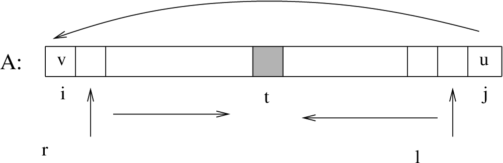
We move a pointer $\mathsf{LeftPtr}$ from location $j$ leftwards (towards $i$ as shown in Figure 1) in order to find an ancestor $w$ of $u$ , which gets added to the end of the queue $\mathsf{ANC}$ . Then we move a pointer $\mathsf{RightPtr}$ from location $i$ rightwards to find a descendant $y$ of $v$ , which gets added to the end of $\mathsf{DES}$ . Then we go back to $\mathsf{LeftPtr}$ , and thus interleave adding a vertex to $\mathsf{ANC}$ with adding a vertex to $\mathsf{DES}$ so that we balance the size of $\mathsf{ANC}$ constructed so far with the size of $\mathsf{DES}$ . When $\mathsf{LeftPtr}$ and $\mathsf{RightPtr}$ meet, that defines our desired location $t$ . We present the detailed algorithm for $\mathsf{Phase}~1$ as Algorithm 2.1. [If $(x,y)\in E$ , we say $x$ is a predecessor of $y$ and $y$ is a successor of $x$ .]

– Initialize

\mathsf{ANC}=\{u\}

and

\mathsf{DES}=\{v\}

– set

\mathsf{RightPtr}=i

and

\mathsf{LeftPtr}=j

. {So

\mathsf{LeftPtr}>\mathsf{RightPtr}

while

\mathsf{TRUE}

\mathsf{LeftPtr}=\mathsf{LeftPtr}-1

;

while

\mathsf{LeftPtr}>\mathsf{RightPtr}

and

A[\mathsf{LeftPtr}]

is not a predecessor of any vertex in

\mathsf{ANC}

\mathsf{LeftPtr}=\mathsf{LeftPtr}-1

;

end while

A[\mathsf{LeftPtr}]

is a predecessor of some vertex in

\mathsf{ANC}

then

– Insert the vertex

A[\mathsf{LeftPtr}]

to the queue

\mathsf{ANC}

end if

\mathsf{LeftPtr}=\mathsf{RightPtr}

then

break {this makes the algorithm break the while

\mathsf{TRUE}

loop}

end if{Now the symmetric process from the side of

v

\mathsf{RightPtr}=\mathsf{RightPtr}+1

;

while

\mathsf{RightPtr}<\mathsf{LeftPtr}

and

A[\mathsf{RightPtr}]

is not a successor of any vertex in

\mathsf{DES}

\mathsf{RightPtr}=\mathsf{RightPtr}+1

;

end while

A[\mathsf{RightPtr}]

is a successor of some vertex in

\mathsf{DES}

then

– Insert the vertex

A[\mathsf{RightPtr}]

to the queue

\mathsf{DES}

end if

\mathsf{RightPtr}=\mathsf{LeftPtr}

then

break

end if{If the algorithm does not break the while

\mathsf{TRUE}

loop, then

\mathsf{LeftPtr}>\mathsf{RightPtr}

end while

Algorithm 2.1 Our algorithm to construct the sets

\mathsf{ANC}

and

\mathsf{DES}

\mathsf{Phase}~1

The above algorithm terminates when $\mathsf{LeftPtr}=\mathsf{RightPtr}$ is satisfied. Set $t$ to be this location: that is, $t=\mathsf{RightPtr}=\mathsf{LeftPtr}$ . It is easy to check that Algorithm 2.1 constructs the sets:

\mathsf{DES}=\{y:i\leq\mathsf{ord}(y)\leq t\ \mathsf{and}\ v\leadsto y\};\ \ \ \mathsf{ANC}=\{w:t\leq\mathsf{ord}(w)\leq j\ \mathsf{and}\ w\leadsto u\}.

That is, $\mathsf{DES}$ is the set of descendants of $v$ in $A[i..t]$ and $\mathsf{ANC}$ is the set of ancestors of $u$ in $A[t..j]$ . The following lemma is straightforward.

Lemma 1

If the new edge $(u,v)$ creates a cycle, then (i) either $A[t]\in\mathsf{DES}\cap\mathsf{ANC}$ or (ii) there is some $x\in\mathsf{DES}$ and $y\in\mathsf{ANC}$ such that there is an edge from $x$ to $y$ .

Proof: If a cycle is created by the insertion of the edge $(u,v)$ , then it implies that $v\leadsto u$ in the current graph. That is, there is a directed path $\rho$ in the graph from $v$ to $u$ , before $(u,v)$ was inserted. This implies that there is either an element in $\mathsf{DES}\cap\mathsf{ANC}$ or there is an edge in $\rho$ that connects a descendant of $v$ in $A[i..t]$ to an ancestor of $u$ in $A[t..j]$ (see Figure 2).

Hence either there is an element in $\mathsf{DES}\cap\mathsf{ANC}$ , the only such element can be $A[t]$ , or there has to be an edge from a vertex in $\mathsf{DES}$ to a vertex in $\mathsf{ANC}$ , where $\mathsf{DES}$ is the set of descendants of $v$ in $A[i..t]$ and $\mathsf{ANC}$ is the set of ancestors of $u$ in $A[t..j]$ .

Lemma 1 shows us that cycle detection is easy, so let us assume henceforth that the edge $(u,v)$ does not create a cycle, hence the graph $G$ is still a DAG. The following lemma shows that the number $t$ has the desired property that we were looking for.

Lemma 2

The number $t$ has the property that the number of descendants of $v$ in $A[i..t]$ is equal to the number of ancestors of $u$ in $A[(t+1)..j]$ .

Proof: We have $t=\mathsf{RightPtr}=\mathsf{LeftPtr}$ . When we terminate the while loop, $\mathsf{ANC}$ is the set of ancestors of $u$ in $A[t..j]$ and $\mathsf{DES}$ is the set of descendants of $v$ from $A[t..j]$ . Since $(u,v)$ does not create a cycle, $A[t]$ is either a descendant of $v$ or an ancestor of $u$ , but not both.

If the main while loop got broken because of the first break statement, then $A[t]$ is a descendant of $v$ and if the main while loop got broken due to the second break statement, then $A[t]$ is an ancestor of $u$ . Since we interleave adding a vertex to the set $\mathsf{ANC}$ with adding a vertex to the set $\mathsf{DES}$ , if we break because of the first break statement, we have $|\mathsf{ANC}|=|\mathsf{DES}|$ ; and if we break because of the second break statement, we have $|\mathsf{ANC}|=|\mathsf{DES}|+1$ . Thus in both cases, it holds that the number of descendants of $v$ in $A[i..t]$ is equal to the number of ancestors of $u$ in $A[(t+1)..j]$ .

At the end of $\mathsf{Phase}~1$ , since $G$ is still a DAG, we delete all the elements of $\mathsf{ANC}\cup\mathsf{DES}$ from their current locations in $A$ . The vertices in $\mathsf{ANC}$ have to find new places in $A[i..t]$ and the vertices in $\mathsf{DES}$ have to find new places in $A[(t+1)..j]$ .²² 2 Note that the number of empty locations in $A[i..t]$ exactly equals $|\mathsf{ANC}|$ and the number of empty locations in $A[(t+1)..j]$ exactly equals $|\mathsf{DES}|$ . This forms $\mathsf{Phase}~2$ of our algorithm.

Phase 2. We now describe $\mathsf{Phase}~2$ from the side of $\mathsf{ANC}$ as Algorithm 2.2. (A symmetric procedure also takes place on the side of $\mathsf{DES}$ .) In this phase vertices get deleted from $\mathsf{ANC}$ and vertices can also get added to $\mathsf{ANC}$ .

\mathsf{LeftPtr}=t

;

while

\mathsf{LeftPtr}\geq i

A[\mathsf{LeftPtr}]

is an empty location then

– delete the head of the queue

\mathsf{ANC}

, call it

h

, and set

A[\mathsf{LeftPtr}]=h

else if

A[\mathsf{LeftPtr}]

(call it

r

) is a predecessor of some element in

\mathsf{ANC}

then

– insert

r

to the queue

\mathsf{ANC}

– delete the head of the queue

\mathsf{ANC}

, call it

h

, and set

A[\mathsf{LeftPtr}]=h

end if

\mathsf{LeftPtr}=\mathsf{LeftPtr}-1

;

end while

Algorithm 2.2

\mathsf{Phase}~2

of our algorithm from the side of

\mathsf{ANC}

In $\mathsf{Phase}~2$ , the pointer $\mathsf{LeftPtr}$ traverses the subarray $A[t..i]$ (from $t$ leftwards to $i$ ) and elements get deleted/inserted in $\mathsf{ANC}$ . Whenever $\mathsf{LeftPtr}$ sees an empty location in $A$ , the head of the queue $\mathsf{ANC}$ is deleted from $\mathsf{ANC}$ and is assigned to that empty location. Whenever $A[\mathsf{LeftPtr}]$ is a predecessor of some element in $\mathsf{ANC}$ , then $A[\mathsf{LeftPtr}]$ is removed from that location and is inserted into $\mathsf{ANC}$ and the current head of the queue $\mathsf{ANC}$ is inserted into that location. We have the following lemma, which is simple to show. Its proof is included in the Appendix.

Lemma 3

The subroutine in Algorithm 2.2 maintains the following invariant in every iteration of the while loop: the number of elements in $\mathsf{ANC}$ equals the number of empty locations in the subarray $A[i..\mathsf{LeftPtr}]$ .

Proof: It is easy to see that the invariant is true at the beginning of the subroutine. In other words, at the end of $\mathsf{Phase}~1$ , the number of empty locations in $A[i..t]$ exactly equals $|\mathsf{ANC}|$ .

We will now show that this invariant is maintained throughout $\mathsf{Phase}~2$ . Whenever $\mathsf{LeftPtr}$ sees an empty location in $A$ , we delete an element from $\mathsf{ANC}$ , hence this invariant is maintained since the number of empty locations in $A[i..\mathsf{LeftPtr}]$ decreases by one and so does the size of $\mathsf{ANC}$ . Whenever $\mathsf{LeftPtr}$ sees a predecessor $p$ of some element of $\mathsf{ANC}$ at the current location, then $p$ is deleted from its current location $\mathsf{LeftPtr}=\ell$ in $A$ and $p$ is inserted into $\mathsf{ANC}$ ; the leading element $h$ of $\mathsf{ANC}$ gets deleted from $\mathsf{ANC}$ and we assign $A[\ell]=h$ . Thus neither the number of empty locations in $A[i..\mathsf{LeftPtr}]$ nor the size of $\mathsf{ANC}$ changes by our deletion and insertion, so the invariant is maintained. Hence when we exit the while loop, which is when $\mathsf{LeftPtr}=i-1$ , the queue $\mathsf{ANC}$ will be empty.

We then traverse the subarray $A[(t+1)..j]$ from location $t+1$ to location $j$ and execute the algorithm in Algorithm 2.2 with respect to $\mathsf{DES}$ . For the sake of completeness, we present that algorithm as Algorithm 2.3 below.

\mathsf{RightPtr}=t+1

;

while

\mathsf{RightPtr}\leq j

A[\mathsf{RightPtr}]

is an empty location then

– delete the head of the queue

\mathsf{DES}

, call it

\ell

, and set

A[\mathsf{RightPtr}]=\ell

else if

A[\mathsf{RightPtr}]

(call it

r

) is a successor of some element in

\mathsf{DES}

then

– insert

r

to the queue

\mathsf{DES}

– delete the head of the queue

\mathsf{DES}

, call it

\ell

, and set

A[\mathsf{RightPtr}]=\ell

end if

\mathsf{RightPtr}=\mathsf{RightPtr}+1

;

end while

Algorithm 2.3

\mathsf{Phase}~2

of our algorithm from the side of

\mathsf{DES}

A lemma analogous to Lemma 3 will show that there is always enough room in the array $A[\mathsf{RightPtr}..j]$ to accommodate the elements of $\mathsf{DES}$ (refer Algorithm 2.3). This completes the description of our algorithm to update the topological ordering when a new edge is inserted.

2.1.2 Correctness.

We would now like to claim that after running $\mathsf{Phase}~1$ and $\mathsf{Phase}~2$ of our algorithm, we have a valid topological ordering. Our ordering is defined in terms of the array $A$ . Each element $x$ that has been assigned a new location in $A$ has a new $\mathsf{ord}$ value, which is the index of its new location. For elements that never belonged to $\mathsf{ANC}\cup\mathsf{DES}$ , the $\mathsf{ord}$ value is unchanged. For the sake of clarity, let us call the ordering before the new edge $(u,v)$ was inserted as $\mathsf{ord}$ and let ${\mathsf{ord}}^{\prime}$ denote the new function after executing our algorithm. We will show the following theorem here (its proof is included in the Appendix).

Theorem 3

The function ${\mathsf{ord}}^{\prime}$ is a valid topological ordering.

Proof: We need to show that $\mathsf{ord}^{\prime}$ is a valid topological ordering. Consider any edge $(x,y)$ in the graph. We will show that ${\mathsf{ord}}^{\prime}(x)<{\mathsf{ord}}^{\prime}(y)$ . We will split this into three cases.

•

$x\in\mathsf{ANC}$ . There are three further cases: (i) $y\in\mathsf{ANC}$ , (ii) $y\in\mathsf{DES}$ , (iii) $y$ is neither in $\mathsf{ANC}$ nor in $\mathsf{DES}$ . In case (i), both $x$ and $y$ are in $\mathsf{ANC}$ and since there is an edge from $x$ to $y$ , the vertex $y$ is ahead of $x$ in the queue $\mathsf{ANC}$ . So $y$ gets deleted from $\mathsf{ANC}$ before $x$ and is hence assigned a higher indexed location in $A$ than $x$ . In other words, ${\mathsf{ord}}^{\prime}(x)<{\mathsf{ord}}^{\prime}(y)$ . In case (ii), we have ${\mathsf{ord}}^{\prime}(x)\leq t<{\mathsf{ord}}^{\prime}(y)$ . In case (iii), since elements of $\mathsf{ANC}$ move to lower indexed locations in $A$ , we have $\mathsf{ord}^{\prime}(x)<\mathsf{ord}(x)$ whereas $\mathsf{ord}^{\prime}(y)=\mathsf{ord}(y)$ ; since ${\mathsf{ord}}(x)<{\mathsf{ord}}(y)$ , we get ${\mathsf{ord}}^{\prime}(x)<{\mathsf{ord}}^{\prime}(y)$ .
•

$x\in\mathsf{DES}$ . There are only two cases here: (i) $y\in\mathsf{DES}$ or (ii) $y$ is neither in $\mathsf{ANC}$ nor in $\mathsf{DES}$ . This is because if $x\in\mathsf{DES}$ and $y\in\mathsf{ANC}$ , then $y\leadsto u\rightarrow v\leadsto x$ . So $(x,y)\in E$ creates a cycle. This is impossible since we assumed that after inserting the edge $(u,v)$ , $G$ remains a DAG. Thus we cannot have $x\in\mathsf{DES}$ and $y\in\mathsf{ANC}$ for $(x,y)\in E$ .

In case (i) here, because $(x,y)\in E$ , the vertex $x$ is ahead of the vertex $y$ in the queue $\mathsf{DES}$ , so $x$ gets deleted from $\mathsf{DES}$ before $y$ and is hence assigned a lower indexed location in $A$ than $y$ . Equivalently, ${\mathsf{ord}}^{\prime}(x)<{\mathsf{ord}}^{\prime}(y)$ . In case (ii) here, since $x\in\mathsf{DES}$ and $y\notin\mathsf{DES}$ , it has to be that either $\mathsf{ord}(y)>\mathsf{ord}(u)$ in which case ${\mathsf{ord}}^{\prime}(x)<{\mathsf{ord}}(y)=\mathsf{ord}^{\prime}(y)$ , or by the time $\mathsf{RightPtr}$ visits the location in $A$ containing $y$ , the vertex $x$ is already deleted from the queue $\mathsf{DES}$ - otherwise, $y$ would have been inserted into $\mathsf{DES}$ . Thus ${\mathsf{ord}}^{\prime}(x)<{\mathsf{ord}}(y)={\mathsf{ord}}^{\prime}(y)$ .
•

$x\notin\mathsf{ANC}\cup\mathsf{DES}$ . There are three cases again here: (i) $y\in\mathsf{ANC}$ , (ii) $y\in\mathsf{DES}$ , (iii) $y$ is neither in $\mathsf{ANC}$ nor in $\mathsf{DES}$ . The arguments here are similar to the earlier arguments and it is easy to check that in all three cases we have ${\mathsf{ord}}^{\prime}(x)<{\mathsf{ord}}^{\prime}(y)$ .

Thus $\mathsf{ord}^{\prime}$ is a valid topological ordering.

Thus our algorithm is correct. In Section 3 we will show that its running time, summed over all edge insertions, is $O(n^{5/2})$ .

3 Running Time Analysis

The main tasks in our algorithm to update $\mathsf{ord}$ to $\mathsf{ord}^{\prime}$ (refer to Algorithms 2.1, 2.2, and 2.3) are:
(1) moving a pointer $\mathsf{LeftPtr}$ from location $j$ to $i$ in the array $A$ and checking if $A[\mathsf{LeftPtr}]$ is a predecessor of any element of $\mathsf{ANC}$ ;
(2) moving a pointer $\mathsf{RightPtr}$ from location $i$ to $j$ in the array $A$ and checking if $A[\mathsf{RightPtr}]$ is a successor of any element of $\mathsf{DES}$ ;
(3) checking at the end of $\mathsf{Phase}~1$ , if $(x,y)\in E$ for any $x$ in $\{x:i\leq\mathsf{ord}(x)\leq t\ \mathsf{and}\ v\leadsto x\}$ and any $y$ in $\{y:t\leq\mathsf{ord}(y)\leq j\ \mathsf{and}\ y\leadsto u\}$ . (If so, then $(u,v)$ creates a cycle.)

Lemma 4 bounds the cost taken by Step 3 over all iterations. It can be proved using a potential function argument.

Lemma 4

The cost for task 3, stated above, summed over all edge insertions, is $O(n^{2})$ .

Proof: We need to check if there is an edge $(x,y)$ between some $x\in\mathsf{DES}$ and some $y\in\mathsf{ANC}$ . We pay a cost of $|\mathsf{ANC}|\cdot|\mathsf{DES}|$ for checking $|\mathsf{ANC}|\cdot|\mathsf{DES}|$ many entries of the matrix $M$ .

Case(i): There is no adjacent pair $(x,y)$ for $x\in\mathsf{DES},y\in\mathsf{ANC}$ . Then the cost $|\mathsf{DES}|\cdot|\mathsf{ANC}|$ can be bounded by $N(e)$ , which is the number of pairs of vertices $(y,x)$ for which the relationship $y\leadsto x$ has started now for the first time (due to the insertion of the edge $(u,v)$ ). Recall that at the end of $\mathsf{Phase}~1$ , $\mathsf{DES}$ is the set $\{x:i\leq\mathsf{ord}(x)\leq t\ \mathsf{and}\ v\leadsto x\}$ and $\mathsf{ANC}$ is the set $\{y:i\leq\mathsf{ord}(y)\leq t\ \mathsf{and}\ y\leadsto u\}$ . Thus each vertex in this set $\mathsf{DES}$ currently has a lower $\mathsf{ord}$ value than each vertex in $\mathsf{ANC}$ - so the only relationship that could have existed between such an $x$ and $y$ is $x\leadsto y$ , which we have ensured does not exist. Thus these pairs $(x,y)$ were incomparable and now the relationship $y\leadsto x$ has been established. It is easy to see that $\sum_{e\in E}N(e)$ is at most $n\choose 2$ since any pair of vertices can contribute at most 1 to $\sum_{e\in E}N(e)$ .

Case(ii): There is indeed an adjacent pair $(x,y)$ for $x\in\mathsf{DES},y\in\mathsf{ANC}$ . Then we quit, since $G$ is no longer a DAG. The check that showed $G$ to contain a cycle cost us $|\mathsf{ANC}|\cdot|\mathsf{DES}|$ , which is $O(n^{2})$ . We pay this cost only once as this is the last step of the algorithm.

Let $\mathsf{ord}_{e}$ be our valid topological ordering before inserting edge $e$ and let $\mathsf{ord}^{\prime}_{e}$ be our valid topological ordering after inserting $e$ . Lemma 5 is our first step in bounding the cost taken for tasks 1 and 2 stated above.

Lemma 5

The cost taken for tasks 1 and 2, stated above, is $\sum_{x\in V}|\mathsf{ord}_{e}(x)-\mathsf{ord}^{\prime}_{e}(x)|$ .

Proof: In Step 1 we find out if $A[\mathsf{LeftPtr}]=x$ is a predecessor of any element of $\mathsf{ANC}$ by checking the entries $M[x,w]$ for each $w\in\mathsf{ANC}$ . Each element $w$ which is currently in $\mathsf{ANC}$ pays unit cost for checking the entry $M[x,w]$ .

Any element $w\in\mathsf{ANC}$ belongs to the set $\mathsf{ANC}$ while $\mathsf{LeftPtr}$ moves from location $\mathsf{ord}_{e}(w)$ to $\mathsf{ord}^{\prime}_{e}(w)$ . When $\mathsf{LeftPtr}=\mathsf{ord}_{e}(w)$ and we identify $A[\mathsf{ord}_{e}(w)]=w$ to be a predecessor of some element in $\mathsf{ANC}$ , the vertex $w$ gets inserted into $\mathsf{ANC}$ . When $\mathsf{LeftPtr}$ is at some empty location $\beta$ and the vertex $w$ is the head of the queue $\mathsf{ANC}$ , then $w$ is deleted from $\mathsf{ANC}$ and we set $A[\beta]=w$ , which implies that $\mathsf{ord}^{\prime}_{e}(w)=\beta$ . So the total cost paid by $w$ is $\mathsf{ord}_{e}(w)-\mathsf{ord}^{\prime}_{e}(w)$ , which is to check the entries $M[A[\mathsf{LeftPtr}],w]$ as the pointer $\mathsf{LeftPtr}$ moves from location $\mathsf{ord}_{e}(w)-1$ to $\mathsf{ord}^{\prime}_{e}(w)$ .

Symmetrically, for any vertex $y$ that belonged to $\mathsf{DES}$ during the course of the algorithm, the cost paid by $y$ is $\mathsf{ord}^{\prime}_{e}(y)-\mathsf{ord}_{e}(y)$ . A vertex $z$ that never belonged to $\mathsf{ANC}\cup\mathsf{DES}$ , does not pay anything and we have $\mathsf{ord}^{\prime}_{e}(z)=\mathsf{ord}_{e}(z)$ . Thus for each $x\in V$ , the cost paid by $x$ to move the pointers $\mathsf{LeftPtr}$ / $\mathsf{RightPtr}$ is $|\mathsf{ord}_{e}(x)-\mathsf{ord}^{\prime}_{e}(x)|$ .

We will show the following result in Section 3.1.

Lemma 6

$\sum_{e\in E}\sum_{x\in V}|\mathsf{ord}_{e}(x)-\mathsf{ord}^{\prime}_{e}(x)|$ is $O(n^{5/2})$ , where $\mathsf{ord}_{e}$ is our valid topological ordering before inserting edge $e$ and $\mathsf{ord}^{\prime}_{e}$ is our valid topological ordering after inserting $e$ .

Theorem 1, stated in Section 1, follows from Theorem 3, Lemmas 4 and 6. Also note that the space requirement of our algorithm is $O(n^{2})$ , since our algorithm uses only the $n\times n$ adjacency matrix $M$ , the array $A$ , the queues $\mathsf{ANC},\mathsf{DES}$ , and the pointers $\mathsf{LeftPtr},\mathsf{RightPtr}$ .

3.1 Proof of Lemma 6

Let $e=(u,v)$ and let $\mathsf{ord}_{e}$ be our topological ordering before inserting $(u,v)$ and $\mathsf{ord}^{\prime}_{e}$ our topological ordering after inserting $(u,v)$ . Our algorithm for updating $\mathsf{ord}_{e}$ to $\mathsf{ord}^{\prime}_{e}$ basically permutes the vertices in the subarray $A[i..j]$ . The elements which get inserted into the queue $\mathsf{ANC}$ move to lower indexed locations in $A$ (compared to their locations in $A$ before $e$ was added), elements which get inserted into the queue $\mathsf{DES}$ move to higher indexed locations in $A$ , and elements which did not get inserted into either $\mathsf{ANC}$ or $\mathsf{DES}$ remain unmoved in $A$ . So our algorithm is essentially a permutation $\pi_{e}$ of elements that belonged to $\mathsf{ANC}\cup\mathsf{DES}$ .

Let ${\mathsf{ANC}}_{e}$ denote the ordered set of all vertices that get inserted to the set $\mathsf{ANC}$ in Algorithms 2.1 and 2.2 (and of course, later get deleted from $\mathsf{ANC}$ in Algorithm 2.2) while inserting the edge $e$ . In other words, these are the vertices $w$ for which $\mathsf{ord}_{e}(w)>\mathsf{ord}^{\prime}_{e}(w)$ . Define $\mathsf{DES}_{e}$ as the ordered set of all those vertices $w$ for which $\mathsf{ord}_{e}(w)<\mathsf{ord}^{\prime}_{e}(w)$ . Equivalently, these are all the vertices that get inserted into $\mathsf{DES}$ in Algorithms 2.1 and 2.3. Let $\mathsf{ANC}_{e}=\{u_{0},u_{1},\ldots,u_{k}\}$ , where $u_{0}=u$ and $\mathsf{ord}(u_{0})>\mathsf{ord}(u_{1})>\cdots>\mathsf{ord}(u_{k})$ , and let $\mathsf{DES}_{e}=\{v_{0},v_{1},\ldots,v_{s}\}$ , where $v_{0}=v$ , and $\mathsf{ord}(v_{0})<\mathsf{ord}(v_{1})<\cdots<\mathsf{ord}(v_{s})$ .

Let us assume that all the vertices of $\mathsf{ANC}_{e}\cup\mathsf{DES}_{e}$ are in their old locations in $A$ (those locations given by the ordering $\mathsf{ord}_{e}$ ; so $A[i]=v$ and $A[j]=u$ ). We will now decompose the permutation $\pi_{e}$ on these elements into a composition of swaps. Note that our algorithm does not perform any swaps, however to prove Lemma 6, it is useful to view $\pi_{e}$ as a composition of appropriate swaps. The function $\mathsf{swap}(x,y)$ takes as input: $x\in\mathsf{ANC}_{e}$ and $y\in\mathsf{DES}_{e}$ , where $\mathsf{ord}(x)>\mathsf{ord}(y)$ , and swaps the occurrences of $x$ and $y$ in the array $A$ . That is, if $A[h]=x$ and $A[\ell]=y$ , where $h>\ell$ , then $\mathsf{swap}(x,y)$ makes $A[\ell]=x$ and $A[h]=y$ .

The intuition behind decomposing $\pi_{e}$ into swaps between such an element $x\in\mathsf{ANC}_{e}$ and such an element $y\in\mathsf{DES}_{e}$ is that we will have the following useful property: whenever we swap two elements $x$ and $y$ , it is always the case that $\mathsf{ord}(x)>\mathsf{ord}(y)$ and we will never swap $x$ and $y$ again in the future (while inserting other new edges) since we now have the relationship $x\leadsto y$ , so $\mathsf{ord}(y)>\mathsf{ord}(x)$ has to hold from now on.

We will use the symbol $\overline{\mathsf{ord}}$ to indicate the dynamic inverse function of $A$ , so that $\overline{\mathsf{ord}}$ reflects instantly changes made in the array $A$ . So as soon as we swap $x$ and $y$ so that $A[\ell]=x$ and $A[h]=y$ , we will say $\overline{\mathsf{ord}}(x)=\ell$ and $\overline{\mathsf{ord}}(y)=h$ . Thus the function $\overline{\mathsf{ord}}$ gets initialized to the function $\mathsf{ord}_{e}$ , it gets updated with every swap that we perform and finally becomes the function $\mathsf{ord}^{\prime}_{e}$ .

3.1.1 3.1.1 Decomposing $\pi_{e}$ into appropriate swaps.

– Initialize the permutation

\pi_{e}

to identity and the function

\overline{\mathsf{ord}}

\mathsf{ord}_{e}

for

x\in\{u_{k},u_{k-1},\ldots,u_{0}\}

(this is

\mathsf{ANC}_{e}

: elements in reverse order of insertion into

\mathsf{ANC}_{e}

) do

for

y\in\{v_{s},v_{s-1},\ldots,v_{0}\}

(this is

\mathsf{DES}_{e}

: elements in reverse order of insertion into

\mathsf{DES}_{e}

) do

\overline{\mathsf{ord}}(x)>\overline{\mathsf{ord}}(y)

then

\pi_{e}=\mathsf{swap}(x,y)\circ\pi_{e}

(

\ast

) {Note that swapping

x

and

y

changes their

\overline{\mathsf{ord}}

values.}

end if

end for

– Return

\pi_{e}

(as a composition of appropriate swaps).

To get a better insight into this decomposition of $\pi_{e}$ , let us take the example of the element $u_{k}\in\mathsf{ANC}$ ( $u_{k}$ has the minimum $\mathsf{ord}_{e}$ value among all the elements in $\mathsf{ANC}$ ). Let $v_{0},v_{1},\ldots,v_{r}$ be the elements of $\mathsf{DES}_{e}$ whose $\mathsf{ord}_{e}$ value is less than $\mathsf{ord}_{e}(u_{k})=\alpha$ . Recall that $\mathsf{ord}_{e}(v_{0})<\cdots<\mathsf{ord}_{e}(v_{r})<\mathsf{ord}_{e}(v_{r+1})<\cdots\mathsf{ord}_{e}(v_{s})$ . When the outer for loop for $x=u_{k}$ is executed, $u_{k}$ does not swap with $v_{s},\ldots,v_{r+1}$ . The first element that $u_{k}$ swaps with is $v_{r}$ , then it swaps with $v_{r-1}$ , so on, and $u_{k}$ finally swaps with $v_{0}$ and takes the location $i$ in $A$ that was occupied by $v_{0}$ . Thus ${\mathsf{ord}}^{\prime}_{e}(u_{k})=i$ and $\overline{\mathsf{ord}}(v_{0}),\ldots,\overline{\mathsf{ord}}(v_{r})$ are higher than what they were formerly, since each $v_{\ell}\in\{v_{0},\ldots,v_{r-1}\}$ is currently occupying the location that was formerly occupied by $v_{\ell+1}$ , and $v_{r}$ is occupying $u_{k}$ ’s old location $\alpha$ . Thus the total movement of $u_{k}$ from location $\alpha$ to location $i$ , can be written as:

\mathsf{ord}_{e}(u_{k})-\mathsf{ord}^{\prime}_{e}(u_{k})=\alpha-i=\sum_{v_{\ell}\in\{v_{r},\ldots,v_{0}\}}d(u_{k},v_{\ell})

where $d(u_{k},v_{\ell})=\overline{\mathsf{ord}}(u_{k})-\overline{\mathsf{ord}}(v_{\ell})$ when $\mathsf{swap}(u_{k},v_{\ell})$ is included in $\pi_{e}$ (refer to ( $\ast$ ) in Section 3.1.1).

Correctness of our decomposition of $\pi_{e}$ .

It is easy to see that the composition of swaps, $\pi_{e}$ , that is returned by the above method in Section 3.1.1, when applied on $\mathsf{ANC}_{e}=\{u_{k},u_{k-1},\ldots,u_{0}\}$ and $\mathsf{DES}_{e}=\{v_{0},\ldots,v_{s-1},v_{s}\}$ , results in these elements occurring in the relative order: $u_{k},u_{k-1},\ldots,$ $u_{0},v_{0},\ldots,v_{s-1},v_{s}$ in $A$ . We claim that our algorithm (Algorithms 2.1, 2.2, 2.3) places these elements in the same order in $A$ . This is because our algorithm maintained both $\mathsf{ANC}$ and $\mathsf{DES}$ as queues - so elements of $\mathsf{ANC}_{e}$ (similarly, $\mathsf{DES}_{e}$ ) do not cross each other, so $u_{k},\ldots,u_{0}$ (resp., $v_{0},\ldots,v_{s}$ ) will be placed in this order, from left to right, in $A$ . Also, we insert all elements of $\mathsf{ANC}_{e}$ in $A[i..t]$ and all elements of $\mathsf{DES}_{e}$ in $A[(t+1)..j]$ , thus our algorithm puts elements of $\mathsf{ANC}_{e}\cup\mathsf{DES}_{e}$ in the order $u_{k},u_{k-1},\ldots,$ $u_{0},v_{0},\ldots,v_{s-1},v_{s}$ in $A$ . Thus we have obtained a correct decomposition (into swaps) of the permutation performed by our algorithm.

For every pair $(x,y)\in\mathsf{ANC}_{e}\times\mathsf{DES}_{e}$ , if $\mathsf{swap}(x,y)$ is included in $\pi_{e}$ (see ( $\ast$ )), define $d(x,y)=\overline{\mathsf{ord}}(x)-\overline{\mathsf{ord}}(y)$ , the difference in the location indices occupied by $x$ and $y$ , when $\mathsf{swap}(x,y)$ gets included in $\pi_{e}$ . For instance, $d(u_{k},v_{0})=\mathsf{ord}_{e}(v_{1})-\mathsf{ord}_{e}(v_{0})$ since $u_{k}$ is in the location $\mathsf{ord}_{e}(v_{1})$ (due to swaps with $v_{r},\ldots,v_{1}$ ) and $v_{0}$ is unmoved in its original location $\mathsf{ord}_{e}(v_{0})$ , at the instant when $\mathsf{swap}(u_{k},v_{0})$ gets included in $\pi_{e}$ .

Since we broke the total movement in $A$ of any $x\in\mathsf{ANC}_{e}$ (which is $\mathsf{ord}_{e}(x)-\mathsf{ord}^{\prime}_{e}(x)$ ) into a sequence of swaps with certain elements in $\mathsf{DES}_{e}$ , we have for any $x\in\mathsf{ANC}_{e}$

\mathsf{ord}_{e}(x)-\mathsf{ord}^{\prime}_{e}(x)=\sum_{y:(x,y)\in\pi_{e}}d(x,y),

where we are using “ $(x,y)\in\pi_{e}$ ” to stand for “ $\mathsf{swap}(x,y)$ exists in $\pi_{e}$ ”.

$\displaystyle\text{We have}\ \sum_{x\in V}\|\mathsf{ord}_{e}(x)-\mathsf{ord}^{\prime}_{e}(x)\|$	$\displaystyle=$	$\displaystyle\sum_{w\in{\mathsf{ANC}}_{e}}(\mathsf{ord}_{e}(w)-\mathsf{ord}^{\prime}_{e}(w))+\sum_{y\in{\mathsf{DES}}_{e}}(\mathsf{ord}^{\prime}_{e}(y)-\mathsf{ord}_{e}(y))$	(1)
	$\displaystyle=$	$\displaystyle 2\sum_{x\in{\mathsf{ANC}}_{e}}(\mathsf{ord}_{e}(x)-\mathsf{ord}^{\prime}_{e}(x))$	(2)
	$\displaystyle=$	$\displaystyle 2\sum_{x\in\mathsf{ANC}_{e}}\ \sum_{y:(x,y)\in\pi_{e}}d(x,y)$	(3)
	$\displaystyle=$	$\displaystyle 2\sum_{(x,y):(x,y)\in\pi_{e}}d(x,y).$	(4)

Equality (2) follows from (1) because $\sum_{x\in V}\mathsf{ord}(x)=\sum_{x\in V}\mathsf{ord}^{\prime}(x)$ . Equality (3) follows from the preceding paragraph. So the entire running time to insert all edges in $E$ is $2\sum_{e\in E}\sum_{(x,y):(x,y)\in\pi_{e}}d(x,y)$ .

We now claim that for any pair $(x,y)$ , we can have $(x,y)\in\pi_{e}$ for at most one permutation $\pi_{e}$ . For $\mathsf{swap}(x,y)$ to exist in $\pi_{e}$ , we need (i) $(x,y)\in\mathsf{ANC}_{e}\times\mathsf{DES}_{e}$ , and (ii) $\mathsf{ord}(x)>\mathsf{ord}(y)$ . Once $\pi_{e}$ swaps $x$ and $y$ , subsequently $x\leadsto y$ (since $x\leadsto u\rightarrow v\leadsto y$ ) and $\mathsf{ord}(y)>\mathsf{ord}(x)$ , so $(x,y)$ can never again satisfy $\mathsf{ord}(x)>\mathsf{ord}(y)$ . So for any pair $(x,y)$ , $\mathsf{swap}(x,y)$ can occur in at most one permutation $\pi_{e}$ over all $e\in E$ . Thus we have:

\sum_{e\in E}\sum_{(x,y):(x,y)\in\pi_{e}}d(x,y)=\sum_{(x,y):(x,y)\in\pi_{e}\ \text{for some $e$}}d(x,y).

(5)

Note that the summation on the right hand side in Inequality (5) is over all those pairs $(x,y)\in V\times V$ such that $\mathsf{swap}(x,y)$ exists in some $\pi_{e}$ , for $e\in E$ .

The following lemma was shown in [1]³³ 3 The algorithm in [1] performs swaps to obtain a valid topological ordering and Lemma 7 is used in their analysis to show an $O(n^{2.75})$ upper bound for the running time of their algorithm.. This finishes the proof of Lemma 6.

Lemma 7

$\sum d(x,y)$ is $O(n^{5/2})$ , where the summation is over all those pairs $(x,y)$ such that $\mathsf{swap}(x,y)$ exists in some permutation $\pi_{e},e\in E$ .

Proof: We present the proof of this lemma given in [1]. We need to show that $\sum_{x,y}d(x,y)$ is $O(n^{5/2})$ . Let $\mathsf{ord}^{*}$ denote the final topological ordering. Define

X(\mathsf{ord}^{*}(x),\mathsf{ord}^{*}(y))=\begin{cases}d(x,y)&\text{if there is some permutation $\pi_{e}$ that swaps $x$ and $y$}\\ 0&\text{otherwise.}\end{cases}

Since $\mathsf{swap}(x,y)$ can occur in at most one permutation $\pi_{e}$ , the variable $X(i,j)$ is clearly defined. Next, we model a few linear constraints on $X(i,j)$ , formulate it as a linear program and use this LP to prove that $\max\{\sum_{i,j}X(i,j)\}=O(n^{5/2})$ . By definition of $d(x,y)$ and $X(i,j)$ ,

0\leq X(i,j)\leq n,\mbox{ for all }i,j\in\{1\ldots n\}.

For $j\leq i$ , the corresponding edges $(\mathsf{ord}^{*-1}(i),\mathsf{ord}^{*-1}(j))$ go backwards and thus are never inserted at all. Consequently,

X(i,j)=0\mbox{ for all }j\leq i.

Now consider an arbitrary vertex $w$ , which is finally at position $i$ , i.e., $\mathsf{ord}^{*}(w)=i$ . Over the insertion of all the edges, this vertex has been moved left and right via swapping with several other vertices. Strictly speaking, it has been swapped left with vertices at final positions $j>i$ and has been swapped right with vertices at final position $j<i$ . Hence, the overall movement to the left is $\sum_{j>i}X(i,j)$ and to the right is $\sum_{j<i}X(j,i)$ . Since the net movement (difference between the final and the initial position) must be less than $n$ ,

\sum_{j>i}X(i,j)-\sum_{j<i}X(j,i)\leq n\mbox{ for all }1\leq i\leq n.

Putting all the constraints together, we aim to solve the following linear program.

\max\sum_{1\leq i\leq n\mbox{, }1\leq j\leq n}X(i,j)\mbox{ such that }

(i)

$X(i,j)=0$ for all $1\leq i\leq n$ and $1\leq j\leq i$
(ii)

$0\leq X(i,j)\leq n$ for all $1\leq i\leq n$ and $i<j\leq n$
(iii)

$\sum_{j>i}X(i,j)-\sum_{j<i}X(j,i)\leq n-1,\mbox{ for all }1\leq i\leq n$

In order to prove the upper bound on the solution to this LP, we consider the dual problem:

\min\left[n\sum_{0\leq i\leq n\mbox{, }i<j<n}Y_{i\cdot n+j}+n\sum_{0\leq i<n}Y_{n^{2}+i}\right]\mbox{ such that}

(i)

$Y_{i\cdot n+j}\geq 1$ for all $0\leq i<n$ and for all $j\leq i$
(ii)

$Y_{i\cdot n+j}+Y_{n^{2}+i}-Y_{n^{2}+j}\geq 1$ for all $0\leq i<n$ and for all $j>i$
(iii)

$Y_{i}\geq 0$ for all $0\leq i<n^{2}+n$

and the following feasible solution for the dual:

$\displaystyle Y_{i\cdot n+j}$	$\displaystyle=$	$\displaystyle 1\mbox{ for all }0\leq i<n\mbox{ and for all }0\leq j\leq i$
$\displaystyle Y_{i\cdot n+j}$	$\displaystyle=$	$\displaystyle 1\mbox{ for all }0\leq i<n\mbox{ and for all }i<j\leq i+1+2\sqrt{n}$
$\displaystyle Y_{i\cdot n+j}$	$\displaystyle=$	$\displaystyle 0\mbox{ for all }0\leq i<n\mbox{ and for all }j>i+1+2\sqrt{n}$
$\displaystyle Y_{n^{2}+i}$	$\displaystyle=$	$\displaystyle\sqrt{n-i}\mbox{ for all }0\leq i<n.$

The solution has a value of $n^{2}+2n^{5/2}+n\sum_{i=1}^{n}\sqrt{i}=O(n^{5/2})$ , which by the primal-dual theorem is a bound on the solution of the original LP. This completes the proof of Lemma 7 and thus Lemma 6 is proved.

4 The $O((m+n\log n)\sqrt{m})$ algorithm

In this section we present an algorithm with running time $O((m+n\log n)\sqrt{m})$ for online topological ordering. This algorithm is an adaptation of the algorithm by Katriel and Bodlaender in [6] and uses the Ordered List data structure from [5], also used in [6] for this problem. That is, the function $\mathsf{ord}$ on $V$ is maintained by a data structure $ORD$ which is a data structure that allows a total order to be maintained over a list of items. Each item $x$ in $ORD$ has an associated integer label $\mathsf{ord}(x)$ and the label associated with $x$ is smaller than the label associated with $y$ , iff $x$ precedes $y$ in the total order. The following operations can be performed in constant amortized time [see Dietz and Sleator [5], Bender et al. [3] for details]: the query Order $(x,y)$ determines whether $x$ precedes $y$ or $y$ precedes $x$ in the total order (i.e., if $\mathsf{ord}(x)<\mathsf{ord}(y)$ or $\mathsf{ord}(y)<\mathsf{ord}(x)$ ), InsertAfter $(x,y)$ (InsertBefore $(x,y)$ ) inserts the item $x$ immediately after (before) the item $y$ in the total order, and Delete $(x)$ removes the item $x$ .

When a new edge ( $u,v$ ) is added to a graph $G$ , there are two cases: (i) either $Order(u,v)$ is true, in which case the current ordering of elements in $ORD$ is still a valid ordering, so we need to do nothing except add $(u,v)$ in the list of edges incoming into $u$ and in the list of edges going out of $v$ ; (ii) $Order(u,v)$ is false, in which case the edge $(u,v)$ is invalidating and we need to change the order of vertices in $ORD$ .

Our algorithm to insert an invalidating edge $(u,v)$ performs various steps. Each step involves visiting an ancestor of $u$ and/or visiting a descendant of $v$ .

$\bullet$ Initially $u$ is the only ancestor of $u$ that we know. So we visit $u$ . We use a Fibonacci heap $F_{u}$ to store ancestors of $u$ that we have seen but not yet visited. For an ancestor $x$ of $u$ , visit( $x$ ) means that for every edge $(w,x)$ into $x$ , we check if $w$ is already present in $F_{u}$ and if $w$ is not present in $F_{u}$ , we insert $w$ into $F_{u}$ .

$\bullet$ The next ancestor of $u$ that we visit is the vertex with the maximum $ORD$ label in $F_{u}$ . An extract-max operation on this F-heap (the priority of vertices in $F_{u}$ is determined by how high their associated label is in $ORD$ ) determines this vertex $x$ .

$\bullet$ Analogously, we have a Fibonacci heap $F_{v}$ to store descendants of $v$ that we have seen but not yet visited. For any descendant $y$ of $v$ , visit( $y$ ) means that for every edge $(y,z)$ out of $y$ , we check if $z$ is already present in the F-heap $F_{v}$ and if $z$ is not present in $F_{v}$ , we insert $z$ into $F_{v}$ . The priority of vertices in $F_{v}$ is determined by how low their associated label is in $ORD$ . Thus an extract-min operation on this F-heap determines the next descendant of $v$ that we visit.

$\bullet$ At the end of each step we check if $Order(x,y)$ is true, where $x$ is the last extracted vertex from $F_{u}$ and $y$ is the last extracted vertex from $F_{v}$ . If $Order(x,y)$ is true (i.e, if $x$ precedes $y$ in $ORD$ ), then this is the termination step; all the ancestors of $u$ that we visited, call them $\{u_{0}(=u),\ldots,u_{k}\}$ and the descendants of $v$ that we visited, call them $\{v_{0}(=v),\ldots,v_{s}\}$ , get reinserted in $ORD$ after $x$ or before $y$ , in the order $u_{k},\ldots,u_{0},v_{0},\ldots,v_{s}$ . Else, i.e, if $y$ precedes $x$ in $ORD$ , then we delete $x$ and $y$ from their current positions in $ORD$ and in the next step we either visit $x$ or $y$ or both $x$ and $y$ .

In any step of the algorithm, if $\{u_{0},u_{1},\ldots,u_{r}\}$ is the set of ancestors of $u$ that we have already visited (in this order, so $\mathsf{ord}(u_{r})<\cdots<\mathsf{ord}(u_{0})$ ) in the previous steps, then the ancestor of $u$ that we plan to visit next is the vertex $x$ with the maximum $ORD$ label that has an edge into a vertex in $\{u_{0},u_{1},\ldots,u_{r}\}$ . Once we visit $x$ , we would have visited all ancestors of $u$ with $ORD$ labels sandwiched between $\mathsf{ord}(x)$ and $\mathsf{ord}(u)$ . Similarly, on the side of $v$ , if $v_{0},v_{1},\ldots,v_{\ell}$ are the descendants of $v$ that we have already visited (i.e., $\mathsf{ord}(v_{0})<\cdots<\mathsf{ord}(v_{\ell})$ ), then the descendant of $v$ that we plan to visit next is the vertex $y$ with the minimum $ORD$ label which has an edge coming from one of $\{v_{0},v_{1},\ldots,v_{\ell}\}$ .

When $Order(x,y)$ is true, it means that we have discovered all descendants of $v$ with $ORD$ label values between $\mathsf{ord}(v)$ and $i$ , and all ancestors of $u$ with $ORD$ label values between $i$ and $\mathsf{ord}(u)$ (where $i$ is any value such that $\mathsf{ord}(x)\leq i\leq\mathsf{ord}(y)$ ). Thus we can relocate vertices $u_{k},\ldots,u_{0},v_{0},\ldots,v_{s}$ (in this order) between $x$ and $y$ . It is easy to see that now for every $(a,b)\in E$ , we have that $a$ precedes $b$ in $ORD$ .

What remains to be explained is how to make the choice between the following 3 options in each step: (i) visit( $x$ ) and visit( $y$ ), (ii) only visit( $x$ ), or (iii) only visit( $y$ ).

Visit( $x$ ) and/or Visit( $y$ ).

In order to make the choice between visit( $x$ ) and/or visit( $y$ ), let us make the following definitions: Let $\mathsf{ANC}$ denote the set of ancestors of $u$ that we have already visited plus the ancestor $x$ that we plan to visit next. Let $\mathsf{DES}$ denote the set of descendants of $v$ that we have already visited plus the descendant $y$ that we plan to visit next. Let $m_{D}$ be the sum of out-degrees of vertices in $\mathsf{DES}$ and let $m_{A}$ be the sum of in-degrees of vertices in $\mathsf{ANC}$ .

If we were to visit $x$ in the current step, then the total work done by us on the side of $u$ so far would be $m_{A}+|\mathsf{ANC}|\log n$ (to have examined $m_{A}$ edges incoming into $\mathsf{ANC}$ and for at most $m_{A}$ insertions in $F_{u}$ , and to have performed $|\mathsf{ANC}|$ many extract-max operations on $F_{u}$ ). Similarly, if we were to visit $y$ in the current step, then the total work done by us on the side of $v$ so far would be $m_{D}+|\mathsf{DES}|\log n$ .

Definition 1

If $m_{A}\leq m_{D}\leq m_{A}+|\mathsf{ANC}|\log{n}$ or $m_{D}\leq m_{A}\leq m_{D}+|\mathsf{DES}|\log{n}$ then we say that $m_{A}$ and $m_{D}$ are “balanced” with respect to each other. Else we say that they are not balanced with respect to each other.

If $m_{A}$ and $m_{D}$ are balanced with respect to each other, then we visit both $x$ and $y$ . Else if $m_{A}<m_{D}$ , then we visit only $x$ , otherwise we visit only $y$ . This is the difference between our algorithm and the algorithm in [6] - in the latter algorithm, either only $x$ is visited or only $y$ is visited unless $m_{D}=m_{A}$ , in which case both $x$ and $y$ are visited. In our algorithm we are ready to visit both $x$ and $y$ more often, that is, whenever $m_{A}$ and $m_{D}$ are “more or less” equal to each other. If we visit both $x$ and $y$ , then the total work done is $m_{A}+|\mathsf{ANC}|\log{n}+m_{D}+|\mathsf{DES}|\log{n}$ . We can give a good upper bound for this quantity using the fact that $m_{A}$ and $m_{D}$ are balanced with respect to each other. On the other hand, if $m_{A}$ and $m_{D}$ are not balanced w.r.t. each other, we are not able to give a good upper bound for the sum of $(m_{A}+|\mathsf{ANC}|\log{n})$ and $(m_{D}+|\mathsf{DES}|\log{n})$ , hence we visit either $x$ or $y$ , depending upon the smaller value in $\{m_{A},m_{D}\}$ .

4.1 The algorithm

Our entire algorithm to reorder vertices in $ORD$ upon the insertion of an invalidating edge $(u,v)$ is described as Algorithm 4.1. This algorithm is basically an implementation of what was described in the previous section with a check at the beginning of every step to see if $m_{A}$ and $m_{D}$ are balanced with respect to each other or not. If they are, then we visit both $x$ and $y$ . Else, we visit only one of them ( $x$ if $m_{A}<m_{D}$ , else $y$ ). The algorithm maintains the invariant that the $ORD$ labels of all elements in $\mathsf{ANC}$ are higher than the $ORD$ labels of all elements in $\mathsf{DES}$ . The termination condition is determined by $Order(x,y)$ being true, where $x$ is the last extracted vertex from $F_{u}$ and $y$ is the last extracted vertex from $F_{v}$ .

For simplicity, in the description of the algorithm we assumed that the heaps $F_{u}$ and $F_{v}$ remain non-empty (otherwise extract-max/extract-min operations would return null values) - handling these cases is easy. We also assumed that the edges inserted are the edges of a DAG. Hence we did not perform any cycle detection here. (Cycle detection can be easily incorporated, by using 2 flags for each vertex that indicate its membership in $F_{u}$ and in $F_{v}$ .) When our algorithm terminates, it is easy to see the order of vertices in $ORD$ is a valid topological ordering. We discuss the running time of Algorithm 4.1 in the next section.

Initially, $\mathsf{ANC}=\{u\}$ and $\mathsf{DES}=\{v\}$ .

Set $x=u$ and $y=v$ . Delete $x$ and $y$ from their current locations in $ORD$ .

Set $m_{A}=u$ ’s in-degree and $m_{D}=v$ ’s out-degree.

while

\mathsf{TRUE}

m_{A}

and

m_{D}

are balanced w.r.t. each other (see Defn. 1) then

Visit(

x

) and Visit(

y

). {So new vertices get inserted into

F_{u}

and into

F_{v}

x=

extract-max(

F_{u}

)

y=

extract-min(

F_{v}

)

\mathsf{ord}(x)<\mathsf{ord}(y)

then

– insert all elements of

\mathsf{ANC}

(with the same relative order within themselves) followed by all elements of

\mathsf{DES}

(with the same relative order) after

x

ORD

break {This terminates the while loop}

else

Delete

x

and

y

from their current positions in

ORD

\mathsf{ANC}=\mathsf{ANC}\cup\{x\}

and

\mathsf{DES}=\mathsf{DES}\cup\{y\}

m_{A}=m_{A}+x

’s in-degree and

m_{D}=m_{D}+y

’s out-degree

end if

else if

m_{A}<m_{D}

then

Visit(

x

)

x=

extract-max(

F_{u}

)

\mathsf{ord}(x)<\mathsf{ord}(y)

then

– insert all elements of

\mathsf{ANC}

followed by all elements of

\mathsf{DES}

after

x

ORD

break

else

Delete

x

from its current position in

ORD

Set

\mathsf{ANC}=\mathsf{ANC}\cup\{x\}

and

m_{A}=m_{A}+x

’s in-degree.

end if

else

Visit(

y

)

Let

y=

extract-max(

F_{v}

)

\mathsf{ord}(x)<\mathsf{ord}(y)

then

– insert all elements of

\mathsf{ANC}

followed by all elements of

\mathsf{DES}

before

y

ORD

break

else

Delete

y

from its current position in

ORD

Set

\mathsf{DES}=\mathsf{DES}\cup\{y\}

and

m_{D}=m_{D}+y

’s out-degree.

end if

end while

Algorithm 4.1 Our algorithm to reorder vertices in

ORD

upon insertion of an invalidating edge

(u,v)

4.1.1 The running time

Let $T(e)$ denote the time taken by Algorithm 4.1 to insert an edge $e$ . We need to show an upper bound for $\sum_{e}T(e)$ , where the sum is over all invalidating edges $e$ . For simplicity of exposition, let us define the following modes. While inserting an edge $(u,v)$ , if a step of our algorithm involved visiting an ancestor of $u$ and a descendant of $v$ , we say that step was performed in mode (i). That is, at the beginning of that step, we had $m_{A}$ and $m_{D}$ balanced with respect to each other. If a step involved visiting only an ancestor of $u$ , then we say that the step was performed in mode (ii), else we say that the step was performed in mode (iii).

We partition the sum $\sum_{e}T(e)$ into 2 parts depending upon the mode of the termination step of our algorithm. Let $S_{1}=\sum_{e}T(e)$ be the time taken by our algorithm over all those edges $e$ such that the termination step was performed in mode (i). Let $S_{2}=\sum_{e}T(e)$ where the sum is over all those edges $e$ such that the termination step was performed in mode (ii) or mode (iii). We will show that both $S_{1}$ and $S_{2}$ are $O((m+n\log n)\sqrt{m})$ . These bounds on $S_{1}$ and $S_{2}$ will prove Theorem 2 stated in Section 1.

The following lemma shows the bound on $S_{1}$ . We then show an analogous bound on $S_{2}$ .

Lemma 8

$S_{1}$ is $O((m+n\log n)\sqrt{m})$ .

Proof: Let us consider any particular edge $e_{i}=(u,v)$ such that the last step of Algorithm 4.1 while inserting $e_{i}$ was performed in mode (i). So the termination step involved visiting an ancestor $u_{k}$ of $u$ , extracting the next ancestor $x$ of $u$ , visiting a descendant $v_{s}$ of $v$ , extracting the next descendant $y$ of $v$ and then checking that $x$ precedes $y$ in $ORD$ .

Let the set $\mathsf{ANC}=\{u,u_{1},\ldots,u_{k}\}$ and the set $\mathsf{DES}=\{v,v_{1},\ldots,v_{s}\}$ . Let $m_{A}$ be the sum of in-degrees of vertices in $\mathsf{ANC}$ and let $m_{D}$ be the sum of out-degrees of vertices in $\mathsf{DES}$ . During all the steps of the algorithm, we extracted $|\mathsf{ANC}|$ many vertices (the vertices $u_{1},\ldots,u_{k}$ and $x$ ) from $F_{u}$ and $|\mathsf{DES}|$ many vertices from $F_{v}$ . So we have $T(e_{i})$ is $O(m_{A}+|\mathsf{ANC}|\log n+m_{D}+|\mathsf{DES}|\log n)$ .

Since the termination step was performed in mode (i), we have that $m_{A}\leq m_{D}\leq m_{A}+|\mathsf{ANC}|\log n$ or $m_{D}\leq m_{A}\leq m_{D}+|\mathsf{DES}|\log n$ . Without loss of generality let us assume that $m_{A}\leq m_{D}\leq m_{A}+|\mathsf{ANC}|\log n$ . Hence $T(e_{i})$ can be upper bounded by some constant times

m_{A}+|\mathsf{ANC}|\log n+|\mathsf{DES}|\log n.

(6)

Let us assume that $|\mathsf{ANC}|>|\mathsf{DES}|$ . (Note that the case $|\mathsf{ANC}|<|\mathsf{DES}|$ is symmetric to this and the case $|\mathsf{ANC}|=|\mathsf{DES}|$ is the easiest.) Since the termination step was performed in mode (i), for $|\mathsf{ANC}|$ to be larger than $|\mathsf{DES}|$ , it must be the case that at some point in the past, our algorithm to insert $e_{i}$ was operating in mode (ii) and that contributed to accumulating quite a few ancestors of $u$ . Let step $t$ be the last step that was operated in mode (ii). So at the beginning of step $t$ we had $m^{\prime}_{A}+|\mathsf{ANC}^{\prime}|\log n\leq m^{\prime}_{D}$ , where $\mathsf{ANC}^{\prime}$ was the set of ancestors of $u$ extracted from the F-heap $F_{u}$ till the beginning of step $t$ and $m^{\prime}_{A}$ is the sum of in-degrees of vertices in $\mathsf{ANC}^{\prime}$ , and $m^{\prime}_{D}$ is the sum of out-degrees of vertices in $\mathsf{DES}^{\prime}$ where $\mathsf{DES}^{\prime}$ was the set of descendants of $v$ extracted from the F-heap $F_{v}$ till the beginning of step $t$ . After step $t$ , we never operated our algorithm in mode (ii). Thus subsequent to step $t$ whenever we extracted a vertex from $F_{u}$ , we also extracted a corresponding vertex from $F_{v}$ . So we have $|\mathsf{ANC}|\leq|\mathsf{ANC}^{\prime}|+|\mathsf{DES}|$ . Using this inequality in (6), we get that

T(e_{i})\leq c(m_{A}+|\mathsf{DES}|\log n+|\mathsf{ANC}^{\prime}|\log n),\ \ \ \text{for some constant $c$}.

Claim 1

We have the following relations:

•

$m_{A}^{2}\leq m_{A}\cdot m_{D}\leq\Phi(e_{i})$

where $\Phi(e_{i})$ is the number of pairs of edges $(e,e^{\prime})$ for which the relationship $e\leadsto e^{\prime}$ has started now for the first time due to the insertion of $e_{i}$ . [We say $(a,b)\leadsto(c,d)$ if $b$ is an ancestor of $c$ .]
•

$|\mathsf{DES}|^{2}\leq|\mathsf{ANC}|\cdot|\mathsf{DES}|\leq N(e_{i})$

where $N(e_{i})$ is the number of pairs of vertices $(w,w^{\prime})$ such that $w\leadsto w^{\prime}$ has started now for the first time due to the insertion of $e_{i}$ . [We say $w\leadsto w^{\prime}$ if $w$ is an ancestor of $w^{\prime}$ .]
•

$(|\mathsf{ANC}^{\prime}|\log n)^{2}\leq(|\mathsf{ANC}^{\prime}|\log n)\cdot m^{\prime}_{D}$ $\leq\Psi(e_{i})\log n$

where $\Psi(e_{i})$ is the number of pairs $(w,e)\in V\times E$ for which the relationship $w\leadsto e$ has started now for the first time. [We say $w\leadsto(a,b)$ if $w$ is an ancestor of $a$ .]

Proof of Claim 1. After the insertion of edge $(u,v)$ we have $e\leadsto e^{\prime}$ for every edge $e$ incoming into $\mathsf{ANC}=\{u,u_{1},\ldots,u_{k}\}$ and every edge $e^{\prime}$ outgoing from $\mathsf{DES}=\{v,v_{1},\ldots,v_{s}\}$ . Prior to inserting $e_{i}$ , the sink of each of the $m_{A}$ edges incoming into $\mathsf{ANC}$ has a higher $ORD$ label compared to the source of each of the $m_{D}$ edges outgoing from $\mathsf{DES}$ - thus we could have had no relation of the form $e\leadsto e^{\prime}$ between the $m_{A}$ edges incoming into $\mathsf{ANC}$ and the $m_{D}$ edges outgoing from $\mathsf{DES}$ . So $\Phi(e_{i})\geq m_{A}m_{D}$ .

The above argument also shows that $N(e_{i})\geq|\mathsf{ANC}|\cdot|\mathsf{DES}|$ . We have $|\mathsf{ANC}^{\prime}|m^{\prime}_{D}\leq\Psi(e_{i})$ because the source of each of these $m^{\prime}_{D}$ edges had a lower $ORD$ label than the vertices in $\mathsf{ANC}^{\prime}$ prior to inserting $e_{i}$ ; thus the relation $w\leadsto e^{\prime}$ for each $w\in\mathsf{ANC}^{\prime}$ and the edges $e^{\prime}$ ( $m^{\prime}_{D}$ many of them) outgoing from $\mathsf{DES}^{\prime}$ is being formed for the first time now.

Now we are ready to finish the proof of Lemma 8. Corresponding to the insertion of each edge $e_{j}$ whose termination step was in mode (i), the work done by our algorithm is at most $c(f_{j}+g_{j}+h_{j})$ where $f_{j}^{2}\leq\Phi(e_{j})$ and $g_{j}^{2}\leq N(e_{j})\log^{2}n$ and $h_{j}^{2}\leq\Psi(e_{j})\log n$ . In order to bound $\sum_{j}(f_{j}+g_{j}+h_{j})$ , we use Cauchy’s inequality which states that $\sum_{i=1}^{m}x_{i}\leq\sqrt{\sum_{i}x^{2}_{i}}\sqrt{m}$ , for $x_{1},\ldots,x_{m}\in\mathbb{R}$ . This yields

$\displaystyle\sum_{j}f_{j}+g_{j}+h_{j}$	$\displaystyle\leq$	$\displaystyle(\sqrt{\sum f_{j}^{2}}+\sqrt{\sum g_{j}^{2}}+\sqrt{\sum h_{j}^{2}})\sqrt{m}$	(7)
	$\displaystyle\leq$	$\displaystyle\left(\sqrt{\sum\Phi(e_{j})}+\sqrt{\sum N(e_{j})}\log n+\sqrt{\sum\Psi(e_{j})\log n}\right)\sqrt{m}$	(8)
	$\displaystyle\leq$	$\displaystyle(m+n\log n+\sqrt{mn\log n})\sqrt{m}.$	(9)

We have $\sum_{j}\Phi(e_{j})$ is at most $m\choose 2$ since each pair of edges $e$ and $e^{\prime}$ can contribute at most 1 to $\sum_{j}\Phi(e_{j})$ ; similarly $\sum_{j}\Psi(e_{j})$ is at most $mn$ , and $\sum_{j}N(e_{j})$ is at most $n\choose 2$ . This yields Inequality (9) from (8). Since $\sqrt{mn\log n}\leq(m+n\log n)/2$ , this completes the proof that the sum $S_{1}$ is $O((m+n\log n)\sqrt{m})$ .

Analogous to Lemma 8, we need to show the following lemma in order to bound the running time of Algorithm 4.1 by $O((m+n\log n)\sqrt{m})$ .

Lemma 9

$S_{2}$ is $O((m+n\log n)\sqrt{m})$ .

Proof: Recall that $S_{2}=\sum T(e)$ where the sum is over all those $e$ such that the termination step of Algorithm 4.1 was performed in mode (ii) or mode (iii). Let us further partition this sum into $\sum_{e}T(e)$ over all those $e$ for which the last step was performed in mode (ii) and $\sum_{e^{\prime}}T(e^{\prime})$ over all those $e^{\prime}$ for which the last step was performed in mode (iii). The analysis for the second sum will be entirely symmetric to the first. We will now bound the first sum.

Let $e_{i}=(u,v)$ be an edge such that the termination step of our algorithm was performed in mode (ii). Let the set $\mathsf{ANC}=\{u,u_{1},\ldots,u_{k}\}$ and let the set $\mathsf{DES}=\{v,v_{1},\ldots,v_{s}\}$ . Let $m_{A}$ be the sum of in-degrees of vertices in $\mathsf{ANC}$ and let $m_{D}$ be the sum of out-degrees of vertices in $\mathsf{DES}$ . Since the termination step was performed in mode (ii), we have $m_{A}+|\mathsf{ANC}|\log n<m_{D}$ .

The work that we did in all the steps while inserting $(u,v)$ from the side of the vertex $u$ is $m_{A}+|\mathsf{ANC}|\log n$ . Let step $t$ be the last step of our algorithm which was operated in mode (i) or in mode (iii). If there was no such step, then the total work done is at most $m_{A}+|\mathsf{ANC}|\log n$ and it is easy to bound this using the inequality $m_{A}+|\mathsf{ANC}|\log n<m_{D}$ . Hence, let us assume that such a step $t$ did exist and let $\mathsf{DES}^{\prime}$ be the set of descendants of $v$ at the beginning of step $t$ and let $m^{\prime}_{D}$ be the sum of out-degrees of vertices in $\mathsf{DES}^{\prime}$ . Note that we have $m^{\prime}_{D}\leq m^{\prime}_{A}+|\mathsf{ANC}^{\prime}|\log n$ since this step was operated in mode (i) or in mode (iii).

The total work done from the side of $v$ is $m^{\prime}_{D}+|\mathsf{DES}^{\prime}|\log n$ . Thus the total work $T(e_{i})$ is $O(m_{A}+|\mathsf{ANC}|\log n+m^{\prime}_{v}+|\mathsf{DES}^{\prime}|\log n)$ . Using the inequality $m^{\prime}_{D}\leq m^{\prime}_{A}+|\mathsf{ANC}^{\prime}|\log n\leq m_{A}+|\mathsf{ANC}|\log n$ , we have $T(e_{i})$ upper bounded by a constant times

m_{A}+|\mathsf{ANC}|\log n+|\mathsf{DES}^{\prime}|\log n.

(10)

Let us concentrate on the last term $|\mathsf{DES}^{\prime}|\log n$ in the above sum. Let $\mathsf{DES}^{\prime\prime}$ be the set of descendants of $v$ at the beginning of the last step when we ran in mode (iii). So $m^{\prime\prime}_{D}+|\mathsf{DES}^{\prime\prime}|\log n\leq m^{\prime\prime}_{A}$ , where $m^{\prime\prime}_{D}$ is the sum of the out-degrees of vertices in $\mathsf{DES}^{\prime\prime}$ , $\mathsf{ANC}^{\prime\prime}$ is the set of ancestors of $u$ at the beginning of this step and $m^{\prime\prime}_{A}$ is the sum of the in-degrees of vertices in $\mathsf{ANC}^{\prime\prime}$ . After this step, whenever we explored edges on the side of $v$ , it was in mode (i), thus visiting a descendant of $v$ was always accompanied by visiting an ancestor of $u$ . So $|\mathsf{DES}^{\prime}|\leq|\mathsf{DES}^{\prime\prime}|+|\mathsf{ANC}|$ . Substituting this bound in (10) we get that

T(e_{i})\leq c(m_{A}+|\mathsf{ANC}|\log n+|\mathsf{DES}^{\prime\prime}|\log n)\ \ \ \text{for some constant $c$}.

We have the following relations (see Claim 1 for the definitions of $\Phi(e_{i})$ and $\Psi(e_{i})$ ):

•

$(m_{A}+|\mathsf{ANC}|\log n)^{2}\leq(m_{A}+|\mathsf{ANC}|\log n)m_{D}$
$\leq\Phi(e_{i})+\Psi(e_{i})\log n$ .
•

$(|\mathsf{DES}^{\prime\prime}|\log n)^{2}\leq(|\mathsf{DES}^{\prime\prime}|\log n)m^{\prime\prime}_{A}$
$\leq\nu(e_{i})\log n$

where $\nu(e_{i})$ is the number of pairs $(e,z)\in E\times V$ that get ordered with respect to each other for the first time now due to the insertion of $e_{i}$ .

The proofs of the above relations are analogous to the proofs given in Claim 1 and we refer the reader to the proof of Claim 1 (in Section 4.1.1).

We are now ready to complete the proof of Lemma 9. $\sum T(e_{i})$ where the sum is over all those $e_{i}$ whose last step was performed in mode (ii) is at most $\sum_{i}(p_{i}+q_{i})$ where $p_{i}^{2}\leq\Phi(e_{i})+\Psi(e_{i})\log n$ and $q_{i}^{2}\leq\nu(e_{i})\log n$ . Note that $\sum_{i}\nu(e_{i})$ is at most $mn$ since each pair $(e,z)\in E\times V$ can contribute at most 1 to $\sum_{i}\nu(e_{i})$ . Using Cauchy’s inequality, we have

$\displaystyle\sum_{i}(p_{i}+q_{i})$	$\displaystyle\leq$	$\displaystyle(\sqrt{\sum p_{i}^{2}}+\sqrt{\sum q_{i}^{2}})\sqrt{m}$
	$\displaystyle\leq$	$\displaystyle\left(\sqrt{\sum\Phi(e_{i})+\sum\Psi(e_{i})\log n}+\sqrt{\sum\nu(e_{i})\log n}\right)\sqrt{m}$
	$\displaystyle\leq$	$\displaystyle(\sqrt{m^{2}+mn\log n}+\sqrt{mn\log n})\sqrt{m}$
	$\displaystyle\leq$	$\displaystyle(m+2\sqrt{mn\log n})\sqrt{m}$

Analogously, we can show that $\sum T(e_{i})$ where the sum is over all those $e_{i}$ whose last step was performed in mode (iii) is at most $O((m+\sqrt{mn\log n})\sqrt{m})$ . Thus $S_{2}$ is $O((m+\sqrt{mn\log n})\sqrt{m})$ . Since $\sqrt{mn\log n}\leq(m+n\log n)/2$ (geometric mean is at most the arithmetic mean), we have $S_{2}$ is $O((m+n\log n)\sqrt{m})$ .

Conclusions.

We considered the problem of maintaining the topological order of a directed acyclic graph on $n$ vertices under an online edge insertion sequence of $m$ edges. This problem has been well-studied and the previous best upper bound for this problem was $O(\min\{m^{3/2}\log n,\ m^{3/2}+n^{2}\log n,\ n^{2.75}\})$ . Here we showed an improved upper bound of $O(\min(n^{5/2},(m+n\log n)\sqrt{m}))$ for this problem.

Acknowledgments.

We are grateful to Deepak Ajwani and Tobias Friedrich for their helpful feedback.

References

[1] D. Ajwani, T. Friedrich, and U. Meyer. An $O(n^{2.75})$ algorithm for online topological ordering. In Proceedings of the 10th Scandinavian Workshop on Algorithm Theory, LNCS 4059: 53-64, 2006. (Longer version in http://arxiv.org/abs/cs/0602073).
[2] B. Alpern, R. Hoover, B. K. Rosen, P. F. Sweeney, and F. K. Zadeck. Incremental evaluation of computational circuits. In Proceedings of the first annual ACM-SIAM Symposium on Discrete Algorithms: 32-42, 1990.
[3] Two simplified algorithms for maintaining order in a list. In Proceedings of the 10th Annual European Symposium on Algorithms: 152-164, 2002.
[4] T. Cormen, C. Leiserson, and R. Rivest. Introduction to Algorithms. The MIT Press, Cambridge, MA, 1989.
[5] P. Dietz and D. Sleator Two algorithms for maintaining order in a list. In Proceedings of the 19th Annual ACM Conference on Theory of Computing: 365-372, 1987.
[6] I. Katriel and H. L. Bodlaender. Online topological ordering. In Proceedings of the 16th ACM-SIAM Symposium on Discrete Algorithms: 443-450, 2005.
[7] A. Marchetti-Spaccamela, U. Nanni, and H. Rohnert. Maintaining a topological order under edge insertions. Information Processing Letters,59(1):53:58,1996.
[8] A. Marchetti-Spaccamela, U. Nanni, and H. Rohnert. On-line graph algorithms for incremental compilation. In Proceedings of the International Workshop on Graph-Theoretic Concepts in Computer Science, LNCS 790: 70-86,1993.
[9] Stephen M. Omohundro, Chu-Cheow Lim, and Jeff Bilmes. The sather language complier/debugger implementation. Technical Report TR-92-017, International Computer Science Institute, Berkeley, 1992.
[10] D.J.Pearce and P.H.J. Kelly. A dynamic algorithm for topologically sorting directed acyclic graphs. In Proceedings of the Workshop on Efficient and Experimental Algorithms, LNCS 3059: 383-398, 2004.
[11] D.J.Pearce, P.H.J. Kelly, and C. Hankin. Online cycle detection and difference propagation for pointer analysis. In Proceedings of the third international IEEE Workshop on Source Code Analysis and Manipulation, 2003.
[12] G. Ramalingam and T. W. Reps. On competitive on-line algorithms for the dynamic priority-ordering problem. Information Processing Letters, 51:155-161, 1994.

Faster Algorithms for Online Topological Ordering

Abstract

1 Introduction

Theorem 1

Theorem 2

1.1 Previous Results

Our Results.

Organization of the paper.

2 The O⁡(n5/2)O(n^{5/2}) Algorithm

2.1 Our algorithm for inserting a new edge (u,v)(u,v) where 𝗈𝗋𝖽⁡(u)>𝗈𝗋𝖽⁡(v)\mathsf{ord}(u)>\mathsf{ord}(v)

2.1.1 Phase 1.

Lemma 1

Lemma 2

Lemma 3

2.1.2 Correctness.

Theorem 3

3 Running Time Analysis

Lemma 4

Lemma 5

Lemma 6

3.1 Proof of Lemma 6

3.1.1 3.1.1 Decomposing πe\pi_{e} into appropriate swaps.

Correctness of our decomposition of πe\pi_{e}.

Lemma 7

4 The O⁡((m+n​log⁡n)​m)O((m+n\log n)\sqrt{m}) algorithm

Visit(xx) and/or Visit(yy).

Definition 1

4.1 The algorithm

4.1.1 The running time

Lemma 8

Claim 1

Lemma 9

Conclusions.

Acknowledgments.

References

2 The $O(n^{5/2})$ Algorithm

2.1 Our algorithm for inserting a new edge $(u,v)$ where $\mathsf{ord}(u)>\mathsf{ord}(v)$

3.1.1 3.1.1 Decomposing $\pi_{e}$ into appropriate swaps.

Correctness of our decomposition of $\pi_{e}$ .

4 The $O((m+n\log n)\sqrt{m})$ algorithm

Visit( $x$ ) and/or Visit( $y$ ).