跳到论文正文
W Papers独立论文阅读器 arXiv:0711.0142 论文正文 计算阅读时间 · 0%
引用这篇论文根据当前论文元数据生成,正式投稿前建议核对。


License: Assumed arXiv.org perpetual non-exclusive license
arXiv:0711.0142v2 [hep-ph] 30 Dec 2007

Collinear and soft gluon corrections to Higgs production at NNNLO

Nikolaos Kidonakis

Kennesaw State University, Physics #1202
1000 Chastain Rd., Kennesaw, GA 30144-5591

Abstract

I present analytical expressions for the collinear and soft gluon corrections to Higgs production via the process b​b¯→Hb{\bar{b}}\rightarrow H as well as g​g→Hgg\rightarrow H through next-to-next-to-next-to-leading order (NNNLO). The soft corrections are complete while the collinear corrections include leading and some subleading logarithms. Numerical results at the Tevatron and the LHC are presented, primarily for b​b¯→Hb{\bar{b}}\rightarrow H. It is shown that the collinear terms greatly improve the soft and virtual approximation at next-to-leading order (NLO) and next-to-next-to-leading order (NNLO), especially when subleading terms are included. The NNNLO collinear and soft corrections provide significant enhancements to the total cross section. I also provide expressions for the collinear and soft corrections through NNNLO for the related Drell-Yan process.

1 Introduction

The search for the Higgs boson [1] is one of the most important goals at the Tevatron and the LHC colliders [2]. The main Standard Model production channel at these colliders is g​g→Hgg\rightarrow H. However, the channel b​b¯→Hb{\bar{b}}\rightarrow H can also be important in the Minimal Supersymmetric Standard Model (MSSM) and other theories beyond the Standard Model. In fact, in the MSSM b​b¯→Hb{\bar{b}}\rightarrow H dominates g​g→Hgg\rightarrow H at high tan⁡β\tan\beta, where tan⁡β\tan\beta is the ratio of the vacuum expectation values for the two Higgs doublets. Complete results through NNLO are known for g​g→Hgg\rightarrow H [3, 4, 5], b​b¯→Hb{\bar{b}}\rightarrow H [6] and the related Drell-Yan processes q​q¯→Vq{\bar{q}}\rightarrow V [7].

Hard-scattering cross sections can receive large corrections from soft-gluon contributions near threshold [8, 9, 10]. Such corrections have been studied for a wide class of cross sections (for a review see [11]) where the soft corrections dominate the cross section. For the process g​g→Hgg\rightarrow H, however, it was shown in [12] that the soft (or even the soft and virtual) corrections are inadequate to serve as a good approximation of the complete cross section at NLO. Collinear corrections have to be added to obtain a reasonable approximation. This was also shown at NNLO in [5]. We verify these results for g​g→Hgg\rightarrow H, and we investigate the soft and collinear approximations for the process b​b¯→Hb{\bar{b}}\rightarrow H. We find that at both NLO and NNLO the soft, or soft and virtual, approximation is inadequate and that collinear logarithms must be added to improve the approximation.

The processes q​q¯→Vq{\bar{q}}\rightarrow V, b​b¯→Hb{\bar{b}}\rightarrow H, and g​g→Hgg\rightarrow H, present a unique opportunity to study complete soft-gluon corrections even at NNNLO. Although partial NNNLO results have appeared for other processes, such as top quark production [13, 14], the complications involved in such processes are far greater. The processes q​q¯→Vq{\bar{q}}\rightarrow V, b​b¯→Hb{\bar{b}}\rightarrow H, and g​g→Hgg\rightarrow H, are much more amenable and easy to study (relative to, for example, heavy quark or jet production) for two distinct reasons:

(i) The color structure of these processes is trivial. At lowest order the processes are electroweak and the final state does not involve any colored particles (quarks or gluons) so the color vertex is trivial. This is to be contrasted with processes such as heavy quark [10] or jet [15] production where the complicated color structure requires matrices in the study of the soft corrections.

(ii) The kinematics of these processes in the calculation of total cross sections are trivial. Again this is to be contrasted with heavy quark or jet production where the kinematics is more complicated and where the structure and form of the soft-gluon terms depends crucially on the kinematics.

It should thus come as no surprise that Drell-Yan and Higgs production are more well understood and known than other hard scattering processes (save deep inelastic scattering).

A unified approach to calculating the soft-gluon corrections for arbitrary hard-scattering processes through NNNLO is available in [13]. We note that related processes involving the Higgs to which the formalism has been applied are charged Higgs production via b​g→t​H−bg\rightarrow tH^{-} [13, 16] and the process b​g→b​Hbg\rightarrow bH [17]. The NNNLO master formula in Ref. [13] is quite long because it is structured so it can address all the possible complications in color structure and kinematics of a general process. Because of the two reasons mentioned above the application of the formula to q​q¯→Vq{\bar{q}}\rightarrow V, b​b¯→Hb{\bar{b}}\rightarrow H, and g​g→Hgg\rightarrow H, results in much simpler expressions.

For the process b​b¯→Hb{\bar{b}}\rightarrow H the complete NNLO corrections were presented in [6]; however the analytic results presented there did not include the scale-dependent terms, and the color structure of the corrections (which is useful to know from a theoretical standpoint and for resummation) was not made explicit. In this paper I present the complete soft-gluon corrections and the collinear logarithms beyond leading accuracy at NLO, NNLO, and NNNLO including the full color factors and the scale-dependent terms. Analytic expressions for the scale-independent terms in the soft-gluon corrections through NNNLO were also presented in Ref. [18] including the full color structure. The results in this paper are in complete agreement with [18].

Studies have been performed on the soft-gluon corrections to the process g​g→Hgg\rightarrow H as well as the Drell-Yan process at NNNLO in [18, 19]. However the analytical results for the scale-dependent terms were not presented. In this paper we derive the full NNNLO soft corrections for g​g→Hgg\rightarrow H and q​q¯→Vq{\bar{q}}\rightarrow V, including explicitly terms with the factorization and renormalization scales, thus verifying and extending the results presented in [18, 19]. Furthermore, we calculate collinear logarithms through NNNLO.

The goals of this paper can be summarized as follows:

(1) For the process b​b¯→Hb{\bar{b}}\rightarrow H: To extend earlier results for the NNLO soft and collinear corrections; to investigate the contribution of soft, virtual, and collinear corrections to the total cross section and determine how well they approximate the complete corrections at NLO and NNLO; to derive at NNNLO the complete soft-gluon corrections and the collinear corrections beyond leading logarithm accuracy; and to provide for the first time a detailed study through NNNLO of the numerical impact of these corrections at the Tevatron and the LHC.

(2) To provide the complete analytical results of the soft-gluon corrections, including scale-dependent terms, and the collinear corrections beyond leading accuracy through NNNLO for the process g​g→Hgg\rightarrow H and for Drell-Yan production. Since these processes have been studied extensively before we do not study numerical applications of the results (except in a limited way for g​g→Hgg\rightarrow H for comparison with b​b¯→Hb{\bar{b}}\rightarrow H).

(3) To study the effects of subleading terms in the soft-gluon expansion and in collinear corrections and make connections with earlier results for various processes.

The paper is organized as follows. In Section 2 we provide a short overview of the formalism for the resummation of soft and collinear logarithms in Higgs and Drell-Yan production. In Section 3 we derive explicit analytical expressions for the soft and collinear corrections for the process b​b¯→Hb{\bar{b}}\rightarrow H. Detailed numerical results are provided in Section 4 for b​b¯→Hb{\bar{b}}\rightarrow H at the Tevatron and the LHC, together with a few results for g​g→Hgg\rightarrow H. The conclusions are in Section 5. Appendix A collects detailed expressions for the numerous quantities needed in the calculations. Appendices B and C contain explicit analytical expressions for the soft and collinear corrections for the Drell-Yan process and for Higgs production via g​g→Hgg\rightarrow H, respectively.

2 Resummation of soft and collinear logarithms

It is well known that soft and collinear logarithms in hard-scattering cross sections exponentiate [8, 9, 10]. In this section we review the resummation formalism for these corrections. The resummation of soft and collinear logarithms is carried out in moment space. We define moments of the partonic cross section by σ^​(N)=∫d​z​zN−1​σ^​(z){\hat{\sigma}}(N)=\int dz\,z^{N-1}{\hat{\sigma}}(z), with z=M2/sz=M^{2}/s. Here MM is a hard scale which we will take to be the Higgs mass mHm_{H} for Higgs production and the invariant mass Q2\sqrt{Q^{2}} of the produced dilepton pair for Drell-Yan production, while s=(p1+p2)2s=(p_{1}+p_{2})^{2} with pip_{i} the momenta of the incoming partons. At partonic threshold, z=1z=1. NN is the moment variable and the logarithms of NN exponentiate. The resummed partonic cross section in moment space can then be written as [13]

σ^r​e​sS​(N)\displaystyle{\hat{\sigma}}_{res}^{S}(N) =\displaystyle= exp[−2∫01dzzN−1−11−z{∫(1−z)21d​λλAi(αs(λM2))+νi[αs((1−z)2M2)]}]\displaystyle\exp\left[-2\int^{1}_{0}dz\frac{z^{N-1}-1}{1-z}\;\left\{\int^{1}_{(1-z)^{2}}\frac{d\lambda}{\lambda}A_{i}\left(\alpha_{s}(\lambda M^{2})\right)+{\nu}_{i}\left[\alpha_{s}((1-z)^{2}M^{2})\right]\right\}\right] (2.1)
×exp⁡[4​∫μFMd​μμ​γi/i​(αs​(μ))]​exp​[2​dαs​∫μRMd​μμ​β​(αs​(μ))]\displaystyle\hskip-62.59605pt\times\,\exp\left[4\int_{\mu_{F}}^{M}\frac{d\mu}{\mu}\;\gamma_{i/i}\left(\alpha_{s}(\mu)\right)\right]\;\exp\left[2d_{\alpha_{s}}\int_{\mu_{R}}^{M}\frac{d\mu}{\mu}\;\beta\left(\alpha_{s}(\mu)\right)\right]\;
×H⁡(αs​(μR))​S​(αs​(M/N~))​exp⁡[2​∫MM/N~d​μμ​ΓS​(αs​(μ))].\displaystyle\hskip-62.59605pt\times\,H\left(\alpha_{s}(\mu_{R})\right)\;S\left(\alpha_{s}(M/{\tilde{N}})\right)\;\exp\left[2\int_{M}^{M/{\tilde{N}}}\frac{d\mu}{\mu}\;\Gamma_{S}\left(\alpha_{s}(\mu)\right)\right]\!.

Factorization-derived resummation studies are based on the above formula or its equivalents. In particular, resummation studies for simple-color-structure processes such as Drell-Yan and Higgs production are based on [8, 9] while processes with more complicated color structure require the additional ingredients in [10, 11, 13, 15].

The expressions for the quantities in the exponents up to three loops are given in Appendix A together with the necessary integrals for NNNLO calculations. The first exponent includes corrections that are universal in hard scattering cross sections and only depends on the identity of the incoming partons (quarks or gluons) [8, 9]. The second and third exponents control the factorization scale, μF\mu_{F}, and the renormalization scale, μR\mu_{R}, dependence of the cross section, respectively. HH is the hard-scattering function for the scattering of partons, while SS is the soft function describing noncollinear soft gluon emission [10]. Also N~=N​eγE{\tilde{N}}=Ne^{\gamma_{E}} where γE\gamma_{E} is the Euler constant. The evolution of the soft function follows from its renormalization group properties and is given in terms of the soft anomalous dimension ΓS\Gamma_{S} which can be explicitly derived through the calculation of eikonal vertex corrections.

To include collinear singularities we essentially replace −2(zN−1−1)/(1−z)-2(z^{N-1}-1)/(1-z) in the first exponent of Eq. (2.1) by 2​zN−12z^{N-1}. These corrections are of the form lnm⁡N/N\ln^{m}N/N in moment space (see Appendix A). The leading collinear corrections come from the one-loop term in AiA_{i} [12, 20]. However at NNLO and beyond one does not derive all the subleading terms from this exponential. We will show, nevertheless, that both analytically and numerically we get the dominant terms and the approximation is excellent.

The exponentials in the resummed cross section can be expanded to any fixed order in the strong coupling αs\alpha_{s} and then inverted to momentum space to provide explicit results for the higher-order corrections. A fixed-order expansion avoids the problems with infrared singularities in the exponents and thus no prescription is needed to deal with these in our approach (see discussion in Ref. [21]). The nn-th order corrections can then be written as

σ^(n)​(z)=V(n)​δ​(1−z)+∑k=02​n−1Sk(n)​[lnk⁡(1−z)1−z]++∑k=02​n−1Ck(n)​lnk⁡(1−z).{\hat{\sigma}}^{(n)}(z)=V^{(n)}\,\delta(1-z)+\sum_{k=0}^{2n-1}S_{k}^{(n)}\left[\frac{\ln^{k}(1-z)}{1-z}\right]_{+}+\sum_{k=0}^{2n-1}C_{k}^{(n)}\ln^{k}(1-z). (2.2)

Here V(n)V^{(n)} are the virtual contributions, the soft contributions are of the form of plus distributions with coefficients Sk(n)S_{k}^{(n)}, and Ck(n)C_{k}^{(n)} are the coefficients of the collinear logarithmic contributions.

To calculate the hadronic cross section we convolute the partonic cross section with parton distribution functions ϕ\phi. The nn-th order corrections to the hadronic cross section can then be written as

σ(n)=τ​∫τ1d​x1​∫τ/x11d​x2​∫01d​z​δ​(τ−x1​x2​z)​ϕ​(x1)​ϕ​(x2)​σ^(n)​(z).\sigma^{(n)}=\tau\int_{\tau}^{1}dx_{1}\int_{\tau/x_{1}}^{1}dx_{2}\int_{0}^{1}dz\;\delta(\tau-x_{1}x_{2}z)\,\phi(x_{1})\,\phi(x_{2})\,{\hat{\sigma}}^{(n)}(z)\,. (2.3)

Here τ=Q2/S\tau=Q^{2}/S and z=Q2/sz=Q^{2}/s for Drell-Yan production, with SS the center-of-mass energy squared of the incoming hadrons, while τ=mH2/S\tau=m_{H}^{2}/S and z=mH2/sz=m_{H}^{2}/s for Higgs production. Substituting the expression of Eq. (2.2) in Eq. (2.3) we have

σ(n)\displaystyle\sigma^{(n)} =\displaystyle= τ∫τ1dx1∫τ/x11dz1x1​zϕ(x1)ϕ(τx1​z){V(n)δ(1−z)+∑k=02​n−1Sk(n)[lnk⁡(1−z)1−z]+\displaystyle\tau\int_{\tau}^{1}dx_{1}\int_{\tau/x_{1}}^{1}dz\,\frac{1}{x_{1}z}\,\phi(x_{1})\,\phi\left(\frac{\tau}{x_{1}z}\right)\left\{V^{(n)}\,\delta(1-z)+\sum_{k=0}^{2n-1}S_{k}^{(n)}\left[\frac{\ln^{k}(1-z)}{1-z}\right]_{+}\right. (2.4)
+∑k=02​n−1Ck(n)lnk(1−z)}\displaystyle\hskip 202.01456pt\left.{}+\sum_{k=0}^{2n-1}C_{k}^{(n)}\ln^{k}(1-z)\right\}

which, after a few manipulations, gives

σ(n)\displaystyle\sigma^{(n)} =\displaystyle= τ∫τ1dx11x1ϕ(x1){ϕ(τx1)[V(n)+∑k=02​n−1Sk(n)k+1lnk+1(1−τx1)]\displaystyle\tau\int_{\tau}^{1}dx_{1}\,\frac{1}{x_{1}}\,\phi(x_{1})\left\{\phi\left(\frac{\tau}{x_{1}}\right)\left[V^{(n)}+\sum_{k=0}^{2n-1}\frac{S_{k}^{(n)}}{k+1}\ln^{k+1}\left(1-\frac{\tau}{x_{1}}\right)\right]\right.
+∫τ/x11dz[1zϕ(τx1​z)−ϕ(τx1)]∑k=02​n−1Sk(n)lnk⁡(1−z)1−z+∫τ/x11dz1zϕ(τx1​z)∑k=02​n−1Ck(n)lnk(1−z)}.\displaystyle\hskip-56.9055pt\left.{}+\int_{\tau/x_{1}}^{1}dz\left[\frac{1}{z}\phi\left(\frac{\tau}{x_{1}z}\right)-\phi\left(\frac{\tau}{x_{1}}\right)\right]\sum_{k=0}^{2n-1}S_{k}^{(n)}\frac{\ln^{k}(1-z)}{1-z}+\int_{\tau/x_{1}}^{1}dz\frac{1}{z}\phi\left(\frac{\tau}{x_{1}z}\right)\sum_{k=0}^{2n-1}C_{k}^{(n)}\ln^{k}(1-z)\right\}\,.

3 Soft and collinear corrections for b​b¯→Hb{\bar{b}}\rightarrow H through NNNLO

In this section we calculate the complete soft-gluon corrections and a large class of collinear corrections beyond leading accuracy to the cross section for the process b​b¯→Hb{\bar{b}}\rightarrow H through NNNLO. In the calculation we also need the virtual corrections through NNLO [6, 18].

We use the notation

Dl​(z)=[lnl⁡(1−z)1−z]+D_{l}(z)=\left[\frac{\ln^{l}(1-z)}{1-z}\right]_{+} (3.1)

to denote the plus distributions in the soft corrections.

The complete NLO soft and virtual corrections are then given by

σ^b​b¯→H(1)​S​V\displaystyle{\hat{\sigma}}^{(1)\,SV}_{b{\bar{b}}\rightarrow H} =\displaystyle= Fb​b¯→HB(μR2)αs​(μR2)π{4CF𝒟1(z)−2CFln(μF2mH2)𝒟0(z)\displaystyle F^{B}_{b{\bar{b}}\rightarrow H}(\mu_{R}^{2})\frac{\alpha_{s}(\mu_{R}^{2})}{\pi}\left\{4C_{F}\,{\cal D}_{1}(z)-2C_{F}\ln\left(\frac{\mu_{F}^{2}}{m_{H}^{2}}\right)\,{\cal D}_{0}(z)\right. (3.2)
+[CF(−1+2ζ2)+32CFln(μR2μF2)]δ(1−z)}\displaystyle\left.{}+\left[C_{F}(-1+2\zeta_{2})+\frac{3}{2}C_{F}\ln\left(\frac{\mu_{R}^{2}}{\mu_{F}^{2}}\right)\right]\,\delta(1-z)\right\}

where the color factors CFC_{F}, CAC_{A} and the ζi\zeta_{i} constants are defined in Appendix A, and the Born term, Fb​b¯→HBF^{B}_{b{\bar{b}}\rightarrow H} is given by

Fb​b¯→HB​(μR2)=π​λb2​(μR2)12​mH2.F^{B}_{b{\bar{b}}\rightarrow H}(\mu_{R}^{2})=\frac{\pi\lambda_{b}^{2}(\mu_{R}^{2})}{12m_{H}^{2}}\,. (3.3)

For the Standard Model process λb​(μR2)=2​mb​(μR2)/v\lambda_{b}(\mu_{R}^{2})=\sqrt{2}m_{b}(\mu_{R}^{2})/v, where v=246v=246 GeV is the Higgs boson vacuum expectation value and mb​(μR2)m_{b}(\mu_{R}^{2}) is the MS¯{\rm\overline{MS}} bottom quark running mass at scale μR\mu_{R}. In the MSSM the value of λb\lambda_{b} depends on which supersymmetric Higgs boson is produced. In the numerical results below we will mostly show ratios of cross sections so the results are equally valid for the Standard Model and the MSSM. However, when values for cross sections are presented in this paper they are always for the Standard Model process.

The leading and next-to-leading collinear corrections at NLO are

σ^b​b¯→H(1)​C=Fb​b¯→HB​(μR2)​αs​(μR2)π​{−4​CF​ln⁡(1−z)+2​CF​ln⁡(μF2mH2)+2​CF}.{\hat{\sigma}}^{(1)\,C}_{b{\bar{b}}\rightarrow H}=F^{B}_{b{\bar{b}}\rightarrow H}(\mu_{R}^{2})\frac{\alpha_{s}(\mu_{R}^{2})}{\pi}\left\{-4C_{F}\,\ln(1-z)+2C_{F}\ln\left(\frac{\mu_{F}^{2}}{m_{H}^{2}}\right)+2C_{F}\right\}\,. (3.4)

The complete NNLO soft and virtual corrections are given by

σ^b​b¯→H(2)​S​V\displaystyle{\hat{\sigma}}^{(2)\,SV}_{b{\bar{b}}\rightarrow H} =\displaystyle= Fb​b¯→HB(μR2)αs2​(μR2)π2{8CF2𝒟3(z)+[−113CFCA+23CFnf−12CF2ln(μF2mH2)]𝒟2(z)\displaystyle F^{B}_{b{\bar{b}}\rightarrow H}(\mu_{R}^{2})\frac{\alpha_{s}^{2}(\mu_{R}^{2})}{\pi^{2}}\left\{8C_{F}^{2}\,{\cal D}_{3}(z)+\left[-\frac{11}{3}C_{F}C_{A}+\frac{2}{3}C_{F}n_{f}-12C_{F}^{2}\ln\left(\frac{\mu_{F}^{2}}{m_{H}^{2}}\right)\right]\,{\cal D}_{2}(z)\right.
+[−4CF2(1+2ζ2)+(679−2ζ2)CFCA−109CFnf+4CF2ln2(μF2mH2)\displaystyle\hskip-28.45274pt{}+\left[-4C_{F}^{2}(1+2\zeta_{2})+\left(\frac{67}{9}-2\zeta_{2}\right)C_{F}C_{A}-\frac{10}{9}C_{F}n_{f}+4C_{F}^{2}\ln^{2}\left(\frac{\mu_{F}^{2}}{m_{H}^{2}}\right)\right.
−6CF2ln(μF2mH2)+CF(6CF+113CA−23nf)ln(μR2mH2)]𝒟1(z)\displaystyle\hskip-28.45274pt\quad\left.{}-6C_{F}^{2}\ln\left(\frac{\mu_{F}^{2}}{m_{H}^{2}}\right)+C_{F}\left(6C_{F}+\frac{11}{3}C_{A}-\frac{2}{3}n_{f}\right)\ln\left(\frac{\mu_{R}^{2}}{m_{H}^{2}}\right)\right]\,{\cal D}_{1}(z)
+[16ζ3CF2+CFCA(−10127+113ζ2+72ζ3)+23CFnf(79−ζ2)\displaystyle\hskip-28.45274pt{}+\left[16\zeta_{3}C_{F}^{2}+C_{F}C_{A}\left(-\frac{101}{27}+\frac{11}{3}\zeta_{2}+\frac{7}{2}\zeta_{3}\right)+\frac{2}{3}C_{F}n_{f}\left(\frac{7}{9}-\zeta_{2}\right)\right.
+CF​(3​CF+1112​CA−nf6)​ln2⁡(μF2mH2)\displaystyle\hskip-28.45274pt\quad{}+C_{F}\left(3C_{F}+\frac{11}{12}C_{A}-\frac{n_{f}}{6}\right)\ln^{2}\left(\frac{\mu_{F}^{2}}{m_{H}^{2}}\right)
+((2+4​ζ2)​CF2+(−6718+ζ2)​CF​CA+59​CF​nf)​ln⁡(μF2mH2)\displaystyle\hskip-28.45274pt\quad{}+\left((2+4\zeta_{2})C_{F}^{2}+(-\frac{67}{18}+\zeta_{2})C_{F}C_{A}+\frac{5}{9}C_{F}n_{f}\right)\ln\left(\frac{\mu_{F}^{2}}{m_{H}^{2}}\right)
−CF(3CF+116CA−nf3)ln(μF2mH2)ln(μR2mH2)]𝒟0(z)\displaystyle\hskip-28.45274pt\quad\left.{}-C_{F}\left(3C_{F}+\frac{11}{6}C_{A}-\frac{n_{f}}{3}\right)\ln\left(\frac{\mu_{F}^{2}}{m_{H}^{2}}\right)\ln\left(\frac{\mu_{R}^{2}}{m_{H}^{2}}\right)\right]\,{\cal D}_{0}(z)
+[CF2(1−154ζ3+ζ2210)+CFCA(8372+2918ζ2−ζ32−320ζ22)+nfCF(118−518ζ2+ζ32)\displaystyle\hskip-28.45274pt{}+\left[C_{F}^{2}\left(1-\frac{15}{4}\zeta_{3}+\frac{\zeta_{2}^{2}}{10}\right)+C_{F}C_{A}\left(\frac{83}{72}+\frac{29}{18}\zeta_{2}-\frac{\zeta_{3}}{2}-\frac{3}{20}\zeta_{2}^{2}\right)+n_{f}C_{F}\left(\frac{1}{18}-\frac{5}{18}\zeta_{2}+\frac{\zeta_{3}}{2}\right)\right.
+(CF2​(98−2​ζ2)+1116​CF​CA−18​CF​nf)​ln2⁡(μF2mH2)\displaystyle\hskip-28.45274pt\quad{}+\left(C_{F}^{2}(\frac{9}{8}-2\zeta_{2})+\frac{11}{16}C_{F}C_{A}-\frac{1}{8}C_{F}n_{f}\right)\ln^{2}\left(\frac{\mu_{F}^{2}}{m_{H}^{2}}\right)
+(CF2​(2116−32​ζ2−11​ζ3)+CF​CA​(−1748−116​ζ2+32​ζ3)+13​CF​nf​(18+ζ2))​ln⁡(μF2mH2)\displaystyle\hskip-28.45274pt\quad{}+\left(C_{F}^{2}(\frac{21}{16}-\frac{3}{2}\zeta_{2}-11\zeta_{3})+C_{F}C_{A}(-\frac{17}{48}-\frac{11}{6}\zeta_{2}+\frac{3}{2}\zeta_{3})+\frac{1}{3}C_{F}n_{f}(\frac{1}{8}+\zeta_{2})\right)\ln\left(\frac{\mu_{F}^{2}}{m_{H}^{2}}\right)
+(−94​CF2−118​CF​CA+14​CF​nf)​ln⁡(μF2mH2)​ln⁡(μR2mH2)\displaystyle\hskip-28.45274pt\quad{}+\left(-\frac{9}{4}C_{F}^{2}-\frac{11}{8}C_{F}C_{A}+\frac{1}{4}C_{F}n_{f}\right)\ln\left(\frac{\mu_{F}^{2}}{m_{H}^{2}}\right)\ln\left(\frac{\mu_{R}^{2}}{m_{H}^{2}}\right)
+(98​CF2+1116​CF​CA−nf8​CF)​ln2⁡(μR2mH2)\displaystyle\hskip-28.45274pt\quad{}+\left(\frac{9}{8}C_{F}^{2}+\frac{11}{16}C_{F}C_{A}-\frac{n_{f}}{8}C_{F}\right)\ln^{2}\left(\frac{\mu_{R}^{2}}{m_{H}^{2}}\right)
+(CF2(−2116+3ζ2)+CFCA(5348+116ζ2)+CFnf(−124−ζ23))ln(μR2mH2)]δ(1−z)},\displaystyle\hskip-28.45274pt\quad\left.\left.{}+\left(C_{F}^{2}\left(-\frac{21}{16}+3\zeta_{2}\right)+C_{F}C_{A}\left(\frac{53}{48}+\frac{11}{6}\zeta_{2}\right)+C_{F}n_{f}\left(-\frac{1}{24}-\frac{\zeta_{2}}{3}\right)\right)\ln\left(\frac{\mu_{R}^{2}}{m_{H}^{2}}\right)\right]\delta(1-z)\right\}\,,

where nfn_{f} is the number of light quark flavors. This is in agreement with Refs. [6, 18].

It is interesting to note here that the scale-independent contribution in the D0D_{0} terms is solely due to ζ3\zeta_{3} terms and the two-loop function Gq​q¯(2)G_{q{\bar{q}}}^{(2)} defined in Appendix A. It was shown in Ref. [22] that for top quark production the inclusion of ζi\zeta_{i} and two-loop Gq​q¯(2)G_{q{\bar{q}}}^{(2)} terms in the D0D_{0} coefficient for that process provided the majority of the D0D_{0} corrections, even though the complete two-loop D0D_{0} terms are not known for that process. This was demonstrated by comparing the corrections in two different kinematics formulations for t​t¯t{\bar{t}} production and showing that the results agree only with the inclusion of these ζi\zeta_{i} and two-loop terms.

The leading and some subleading collinear corrections at NNLO are

σ^b​b¯→H(2)​C\displaystyle{\hat{\sigma}}^{(2)\,C}_{b{\bar{b}}\rightarrow H} =\displaystyle= Fb​b¯→HB(μR2)αs2​(μR2)π2{−8CF2ln3(1−z)\displaystyle F^{B}_{b{\bar{b}}\rightarrow H}(\mu_{R}^{2})\frac{\alpha_{s}^{2}(\mu_{R}^{2})}{\pi^{2}}\left\{-8C_{F}^{2}\,\ln^{3}(1-z)\right. (3.6)
+[12​CF2+113​CF​CA−23​CF​nf+12​CF2​ln⁡(μF2mH2)]​ln2⁡(1−z)\displaystyle\hskip-28.45274pt{}+\left[12C_{F}^{2}+\frac{11}{3}C_{F}C_{A}-\frac{2}{3}C_{F}n_{f}+12C_{F}^{2}\ln\left(\frac{\mu_{F}^{2}}{m_{H}^{2}}\right)\right]\,\ln^{2}(1-z)
+[4CF2(1+2ζ2)+CFCA(2ζ2−1009)+169nfCF−4CF2ln2(μF2mH2)\displaystyle\hskip-28.45274pt{}+\left[4C_{F}^{2}(1+2\zeta_{2})+C_{F}C_{A}\left(2\zeta_{2}-\frac{100}{9}\right)+\frac{16}{9}n_{f}C_{F}-4C_{F}^{2}\ln^{2}\left(\frac{\mu_{F}^{2}}{m_{H}^{2}}\right)\right.
−CF(113CA−23nf)ln(μR2mH2)−6CF2ln(μF2mH2)−6CF2ln(μR2mH2)]ln(1−z)\displaystyle\hskip-14.22636pt\left.{}-C_{F}\left(\frac{11}{3}C_{A}-\frac{2}{3}n_{f}\right)\ln\left(\frac{\mu_{R}^{2}}{m_{H}^{2}}\right)-6C_{F}^{2}\ln\left(\frac{\mu_{F}^{2}}{m_{H}^{2}}\right)-6C_{F}^{2}\ln\left(\frac{\mu_{R}^{2}}{m_{H}^{2}}\right)\right]\,\ln(1-z)
−CF​(CF+1112​CA−nf6)​ln2⁡(μF2mH2)+CF​(3​CF+116​CA−13​nf)​ln⁡(μF2mH2)​ln⁡(μR2mH2)\displaystyle\hskip-28.45274pt{}-C_{F}\left(C_{F}+\frac{11}{12}C_{A}-\frac{n_{f}}{6}\right)\ln^{2}\left(\frac{\mu_{F}^{2}}{m_{H}^{2}}\right)+C_{F}\left(3C_{F}+\frac{11}{6}C_{A}-\frac{1}{3}n_{f}\right)\ln\left(\frac{\mu_{F}^{2}}{m_{H}^{2}}\right)\ln\left(\frac{\mu_{R}^{2}}{m_{H}^{2}}\right)
+(−5​CF2+6718​CF​CA−4​CF2​ζ2−CF​CA​ζ2−59​nf​CF)​ln⁡(μF2mH2)\displaystyle\hskip-28.45274pt{}+\left(-5C_{F}^{2}+\frac{67}{18}C_{F}C_{A}-4C_{F}^{2}\zeta_{2}-C_{F}C_{A}\zeta_{2}-\frac{5}{9}n_{f}C_{F}\right)\ln\left(\frac{\mu_{F}^{2}}{m_{H}^{2}}\right)
+CF(3CF+116CA−13nf)ln(μR2mH2)}.\displaystyle\hskip-28.45274pt\left.{}+C_{F}\left(3C_{F}+\frac{11}{6}C_{A}-\frac{1}{3}n_{f}\right)\ln\left(\frac{\mu_{R}^{2}}{m_{H}^{2}}\right)\right\}\,.

Several remarks are in order here. The leading collinear (LC) logarithms at NNLO (i.e. ln3⁡(1−z)\ln^{3}(1-z)) are complete. The next-to-leading collinear (NLC) logarithms (i.e ln2⁡(1−z)\ln^{2}(1-z)) are not complete. However, numerically they are an excellent approximation to the complete NLC terms. Also analytically the CF​CAC_{F}C_{A}, nf​CFn_{f}C_{F} and the ln⁡(μF2/mH2)\ln(\mu_{F}^{2}/m_{H}^{2}) terms are exact. The next-to-next-to-leading collinear (NNLC) logarithms (i.e ln⁡(1−z)\ln(1-z)) are also not complete. However, again numerically they are an excellent approximation to the complete NNLC terms. Also analytically the CF2​ζ2C_{F}^{2}\zeta_{2}, CF​CA​ζ2C_{F}C_{A}\zeta_{2}, ln2⁡(μF2/mH2)\ln^{2}(\mu_{F}^{2}/m_{H}^{2}), and ln⁡(μR2/mH2)\ln(\mu_{R}^{2}/m_{H}^{2}) terms are exact. Finally, in the constant terms we only show the scale-dependent terms; the ln2⁡(μF2/mH2)\ln^{2}(\mu_{F}^{2}/m_{H}^{2}), ln⁡(μF2/mH2)​ln⁡(μR2/mH2)\ln(\mu_{F}^{2}/m_{H}^{2})\ln(\mu_{R}^{2}/m_{H}^{2}) and ln⁡(μR2/mH2)\ln(\mu_{R}^{2}/m_{H}^{2}) terms are exact, while the ln⁡(μF2/mH2)\ln(\mu_{F}^{2}/m_{H}^{2}) terms are almost exact. More details on the numerical approximation are given in Section 4, and on the analytical approximation in the context of the related Drell-Yan process, where explicit results involving the color factors have been published [7], in Appendix B.

The complete NNNLO soft-gluon corrections are given by

σ^b​b¯→H(3)​S\displaystyle{\hat{\sigma}}^{(3)\,S}_{b{\bar{b}}\rightarrow H} =\displaystyle= Fb​b¯→HB(μR2)αs3​(μR2)π3{8CF3𝒟5(z)+[−1109CF2CA+209CF2nf−20CF3ln(μF2mH2)]𝒟4(z)\displaystyle F^{B}_{b{\bar{b}}\rightarrow H}(\mu_{R}^{2})\frac{\alpha_{s}^{3}(\mu_{R}^{2})}{\pi^{3}}\;\left\{8C_{F}^{3}\;{\cal D}_{5}(z)+\left[-\frac{110}{9}C_{F}^{2}C_{A}+\frac{20}{9}C_{F}^{2}n_{f}-20C_{F}^{3}\ln\left(\frac{\mu_{F}^{2}}{m_{H}^{2}}\right)\right]\;{\cal D}_{4}(z)\right. (3.7)
+[−8CF3(1+6ζ2)+CF2CA(2689−8ζ2)+12127CFCA2−409CF2nf−4427CFCAnf+427CFnf2\displaystyle\hskip-42.67912pt{}+\left[-8C_{F}^{3}(1+6\zeta_{2})+C_{F}^{2}C_{A}\left(\frac{268}{9}-8\zeta_{2}\right)+\frac{121}{27}C_{F}C_{A}^{2}-\frac{40}{9}C_{F}^{2}n_{f}-\frac{44}{27}C_{F}C_{A}n_{f}+\frac{4}{27}C_{F}n_{f}^{2}\right.
+16​CF3​ln2⁡(μF2mH2)+(−12​CF3+889​CF2​CA−169​CF2​nf)​ln⁡(μF2mH2)\displaystyle\hskip-28.45274pt{}+16C_{F}^{3}\ln^{2}\left(\frac{\mu_{F}^{2}}{m_{H}^{2}}\right)+\left(-12C_{F}^{3}+\frac{88}{9}C_{F}^{2}C_{A}-\frac{16}{9}C_{F}^{2}n_{f}\right)\ln\left(\frac{\mu_{F}^{2}}{m_{H}^{2}}\right)
+(12CF3+443CF2CA−83CF2nf)ln(μR2mH2)]𝒟3(z)\displaystyle\hskip-28.45274pt\left.{}+\left(12C_{F}^{3}+\frac{44}{3}C_{F}^{2}C_{A}-\frac{8}{3}C_{F}^{2}n_{f}\right)\ln\left(\frac{\mu_{R}^{2}}{m_{H}^{2}}\right)\right]\;{\cal D}_{3}(z)
+[160ζ3CF3+CF2CA(−1699+1763ζ2+21ζ3)+CFCA2(−44527+113ζ2)+CF2nf(5318−323ζ2)\displaystyle\hskip-42.67912pt{}+\left[160\zeta_{3}C_{F}^{3}+C_{F}^{2}C_{A}\left(-\frac{169}{9}+\frac{176}{3}\zeta_{2}+21\zeta_{3}\right)+C_{F}C_{A}^{2}\left(-\frac{445}{27}+\frac{11}{3}\zeta_{2}\right)+C_{F}^{2}n_{f}\left(\frac{53}{18}-\frac{32}{3}\zeta_{2}\right)\right.
+CF​CA​nf​(28954−23​ζ2)−1027​CF​nf2−4​CF3​ln3⁡(μF2mH2)+CF2​(18​CF+112​CA−nf)​ln2⁡(μF2mH2)\displaystyle\hskip-28.45274pt{}+C_{F}C_{A}n_{f}\left(\frac{289}{54}-\frac{2}{3}\zeta_{2}\right)-\frac{10}{27}C_{F}n_{f}^{2}-4C_{F}^{3}\ln^{3}\left(\frac{\mu_{F}^{2}}{m_{H}^{2}}\right)+C_{F}^{2}\left(18C_{F}+\frac{11}{2}C_{A}-n_{f}\right)\ln^{2}\left(\frac{\mu_{F}^{2}}{m_{H}^{2}}\right)
+(12​(1+6​ζ2)​CF3+(−2356+12​ζ2)​CF2​CA+173​CF2​nf)​ln⁡(μF2mH2)\displaystyle\hskip-28.45274pt{}+\left(12(1+6\zeta_{2})C_{F}^{3}+(-\frac{235}{6}+12\zeta_{2})C_{F}^{2}C_{A}+\frac{17}{3}C_{F}^{2}n_{f}\right)\ln\left(\frac{\mu_{F}^{2}}{m_{H}^{2}}\right)
+(−18​CF3−22​CF2​CA+4​CF2​nf)​ln⁡(μF2mH2)​ln⁡(μR2mH2)\displaystyle\hskip-28.45274pt{}+(-18C_{F}^{3}-22C_{F}^{2}C_{A}+4C_{F}^{2}n_{f})\ln\left(\frac{\mu_{F}^{2}}{m_{H}^{2}}\right)\ln\left(\frac{\mu_{R}^{2}}{m_{H}^{2}}\right)
+(−112CF2CA−12118CFCA2+CF2nf+229CFCAnf−29CFnf2)ln(μR2mH2)]𝒟2(z)\displaystyle\hskip-28.45274pt\left.{}+\left(-\frac{11}{2}C_{F}^{2}C_{A}-\frac{121}{18}C_{F}C_{A}^{2}+C_{F}^{2}n_{f}+\frac{22}{9}C_{F}C_{A}n_{f}-\frac{2}{9}C_{F}n_{f}^{2}\right)\ln\left(\frac{\mu_{R}^{2}}{m_{H}^{2}}\right)\right]{\cal D}_{2}(z)
+[CF3(4+16ζ2−15ζ3−192ζ4+1625ζ22)+CF2CA(−176−3269ζ2−90ζ3+575ζ22)\displaystyle\hskip-42.67912pt{}+\left[C_{F}^{3}\left(4+16\zeta_{2}-15\zeta_{3}-192\zeta_{4}+\frac{162}{5}\zeta_{2}^{2}\right)+C_{F}^{2}C_{A}\left(-\frac{17}{6}-\frac{326}{9}\zeta_{2}-90\zeta_{3}+\frac{57}{5}\zeta_{2}^{2}\right)\right.
+CF​CA2​(15503648−1889​ζ2−11​ζ3+115​ζ22)+CF2​nf​(−2324+509​ζ2+20​ζ3)\displaystyle\hskip-28.45274pt{}+C_{F}C_{A}^{2}\left(\frac{15503}{648}-\frac{188}{9}\zeta_{2}-11\zeta_{3}+\frac{11}{5}\zeta_{2}^{2}\right)+C_{F}^{2}n_{f}\left(-\frac{23}{24}+\frac{50}{9}\zeta_{2}+20\zeta_{3}\right)
+CF​CA​nf​(−2051324+6​ζ2)+CF​nf2​(2581−49​ζ2)\displaystyle\hskip-28.45274pt{}+C_{F}C_{A}n_{f}\left(-\frac{2051}{324}+6\zeta_{2}\right)+C_{F}n_{f}^{2}\left(\frac{25}{81}-\frac{4}{9}\zeta_{2}\right)
+(−6​CF3−113​CF2​CA+23​CF2​nf)​ln3⁡(μF2mH2)\displaystyle\hskip-28.45274pt{}+\left(-6C_{F}^{3}-\frac{11}{3}C_{F}^{2}C_{A}+\frac{2}{3}C_{F}^{2}n_{f}\right)\ln^{3}\left(\frac{\mu_{F}^{2}}{m_{H}^{2}}\right)
+((12−32​ζ2)​CF3+(63536−4​ζ2)​CF2​CA−4918​CF2​nf)​ln2⁡(μF2mH2)\displaystyle\hskip-28.45274pt{}+\left((\frac{1}{2}-32\zeta_{2})C_{F}^{3}+(\frac{635}{36}-4\zeta_{2})C_{F}^{2}C_{A}-\frac{49}{18}C_{F}^{2}n_{f}\right)\ln^{2}\left(\frac{\mu_{F}^{2}}{m_{H}^{2}}\right)
+CF2​(6​CF+223​CA−43​nf)​ln2⁡(μF2mH2)​ln⁡(μR2mH2)\displaystyle\hskip-28.45274pt{}+C_{F}^{2}\left(6C_{F}+\frac{22}{3}C_{A}-\frac{4}{3}n_{f}\right)\ln^{2}\left(\frac{\mu_{F}^{2}}{m_{H}^{2}}\right)\ln\left(\frac{\mu_{R}^{2}}{m_{H}^{2}}\right)
+CF2​(−9​CF−11​CA+2​nf)​ln⁡(μF2mH2)​ln⁡(μR2mH2)\displaystyle\hskip-28.45274pt{}+C_{F}^{2}(-9C_{F}-11C_{A}+2n_{f})\ln\left(\frac{\mu_{F}^{2}}{m_{H}^{2}}\right)\ln\left(\frac{\mu_{R}^{2}}{m_{H}^{2}}\right)
+((214+18​ζ2−172​ζ3)​CF3+(257108−1013​ζ2−8​ζ3)​CF2​CA+(−1354+203​ζ2)​CF2​nf)​ln⁡(μF2mH2)\displaystyle\hskip-28.45274pt{}+\left((\frac{21}{4}+18\zeta_{2}-172\zeta_{3})C_{F}^{3}+(\frac{257}{108}-\frac{101}{3}\zeta_{2}-8\zeta_{3})C_{F}^{2}C_{A}+(-\frac{13}{54}+\frac{20}{3}\zeta_{2})C_{F}^{2}n_{f}\right)\ln\left(\frac{\mu_{F}^{2}}{m_{H}^{2}}\right)
+(92​CF3+334​CF2​CA+12136​CF​CA2−32​nf​CF2−119​CF​CA​nf+19​CF​nf2)​ln2⁡(μR2mH2)\displaystyle\hskip-28.45274pt{}+\left(\frac{9}{2}C_{F}^{3}+\frac{33}{4}C_{F}^{2}C_{A}+\frac{121}{36}C_{F}C_{A}^{2}-\frac{3}{2}n_{f}C_{F}^{2}-\frac{11}{9}C_{F}C_{A}n_{f}+\frac{1}{9}C_{F}n_{f}^{2}\right)\ln^{2}\left(\frac{\mu_{R}^{2}}{m_{H}^{2}}\right)
+(CF3​(−214−12​ζ2)+(14312−533​ζ2)​CF2​CA+(44527−113​ζ2)​CF​CA2+13​(−5+8​ζ2)​CF2​nfCLOSE\displaystyle\hskip-28.45274pt{}+\left(C_{F}^{3}\left(-\frac{21}{4}-12\zeta_{2}\right)+\left(\frac{143}{12}-\frac{53}{3}\zeta_{2}\right)C_{F}^{2}C_{A}+(\frac{445}{27}-\frac{11}{3}\zeta_{2})C_{F}C_{A}^{2}+\frac{1}{3}(-5+8\zeta_{2})C_{F}^{2}n_{f}\right.
+(−28954+23ζ2)CFCAnf+1027CFnf2)ln(μR2mH2)]𝒟1(z)\displaystyle\left.\left.{}+(-\frac{289}{54}+\frac{2}{3}\zeta_{2})C_{F}C_{A}n_{f}+\frac{10}{27}C_{F}n_{f}^{2}\right)\ln\left(\frac{\mu_{R}^{2}}{m_{H}^{2}}\right)\right]\;{\cal D}_{1}(z)
+[CF3(−16ζ3+192ζ5−96ζ2ζ3)+CF2CA(10127+10327ζ2+100918ζ3+2203ζ4−22ζ22−23ζ2ζ3)\displaystyle\hskip-42.67912pt{}+\left[C_{F}^{3}(-16\zeta_{3}+192\zeta_{5}-96\zeta_{2}\zeta_{3})+C_{F}^{2}C_{A}\left(\frac{101}{27}+\frac{103}{27}\zeta_{2}+\frac{1009}{18}\zeta_{3}+\frac{220}{3}\zeta_{4}-22\zeta_{2}^{2}-23\zeta_{2}\zeta_{3}\right)\right.
+CF​CA2​(−29702923328+6139324​ζ2+2509108​ζ3−6​ζ5−18760​ζ22−116​ζ2​ζ3)\displaystyle\hskip-28.45274pt{}+C_{F}C_{A}^{2}\left(-\frac{297029}{23328}+\frac{6139}{324}\zeta_{2}+\frac{2509}{108}\zeta_{3}-6\zeta_{5}-\frac{187}{60}\zeta_{2}^{2}-\frac{11}{6}\zeta_{2}\zeta_{3}\right)
+CF2​nf​(421288−4754​ζ2−17918​ζ3−403​ζ4+195​ζ22)+CF​CA​nf​(3131311664−1837324​ζ2−15536​ζ3+2330​ζ22)\displaystyle\hskip-28.45274pt{}+C_{F}^{2}n_{f}\left(\frac{421}{288}-\frac{47}{54}\zeta_{2}-\frac{179}{18}\zeta_{3}-\frac{40}{3}\zeta_{4}+\frac{19}{5}\zeta_{2}^{2}\right)+C_{F}C_{A}n_{f}\left(\frac{31313}{11664}-\frac{1837}{324}\zeta_{2}-\frac{155}{36}\zeta_{3}+\frac{23}{30}\zeta_{2}^{2}\right)
+CF​nf2​(−58729+1027​ζ2+527​ζ3)\displaystyle\hskip-28.45274pt{}+C_{F}n_{f}^{2}\left(-\frac{58}{729}+\frac{10}{27}\zeta_{2}+\frac{5}{27}\zeta_{3}\right)
+((−94+4​ζ2)​CF3−114​CF2​CA−121216​CF​CA2+12​CF2​nf+1154​CF​CA​nf−154​CF​nf2)​ln3⁡(μF2mH2)\displaystyle\hskip-28.45274pt{}+\left((-\frac{9}{4}+4\zeta_{2})C_{F}^{3}-\frac{11}{4}C_{F}^{2}C_{A}-\frac{121}{216}C_{F}C_{A}^{2}+\frac{1}{2}C_{F}^{2}n_{f}+\frac{11}{54}C_{F}C_{A}n_{f}-\frac{1}{54}C_{F}n_{f}^{2}\right)\ln^{3}\left(\frac{\mu_{F}^{2}}{m_{H}^{2}}\right)
+((−218−9​ζ2+38​ζ3)​CF3+(438+ζ23−3​ζ3)​CF2​CA+(445108−1112​ζ2)​CF​CA2CLOSE\displaystyle\hskip-28.45274pt{}+\left((-\frac{21}{8}-9\zeta_{2}+38\zeta_{3})C_{F}^{3}+(\frac{43}{8}+\frac{\zeta_{2}}{3}-3\zeta_{3})C_{F}^{2}C_{A}+(\frac{445}{108}-\frac{11}{12}\zeta_{2})C_{F}C_{A}^{2}\right.
OPEN+(−78−ζ23)​CF2​nf+(−289216+ζ26)​CF​CA​nf+554​CF​nf2)​ln2⁡(μF2mH2)\displaystyle\hskip-28.45274pt\left.{}+(-\frac{7}{8}-\frac{\zeta_{2}}{3})C_{F}^{2}n_{f}+(-\frac{289}{216}+\frac{\zeta_{2}}{6})C_{F}C_{A}n_{f}+\frac{5}{54}C_{F}n_{f}^{2}\right)\ln^{2}\left(\frac{\mu_{F}^{2}}{m_{H}^{2}}\right)
+(92​CF3+558​CF2​CA+12172​CF​CA2−54​CF2​nf−1118​CF​CA​nf+118​CF​nf2)​ln2⁡(μF2mH2)​ln⁡(μR2mH2)\displaystyle\hskip-28.45274pt{}+\left(\frac{9}{2}C_{F}^{3}+\frac{55}{8}C_{F}^{2}C_{A}+\frac{121}{72}C_{F}C_{A}^{2}-\frac{5}{4}C_{F}^{2}n_{f}-\frac{11}{18}C_{F}C_{A}n_{f}+\frac{1}{18}C_{F}n_{f}^{2}\right)\ln^{2}\left(\frac{\mu_{F}^{2}}{m_{H}^{2}}\right)\ln\left(\frac{\mu_{R}^{2}}{m_{H}^{2}}\right)
+(−94​CF3−338​CF2​CA−12172​CF​CA2+34​nf​CF2+1118​CF​CA​nf−118​CF​nf2)​ln⁡(μF2mH2)​ln2⁡(μR2mH2)\displaystyle\hskip-28.45274pt{}+\left(-\frac{9}{4}C_{F}^{3}-\frac{33}{8}C_{F}^{2}C_{A}-\frac{121}{72}C_{F}C_{A}^{2}+\frac{3}{4}n_{f}C_{F}^{2}+\frac{11}{18}C_{F}C_{A}n_{f}-\frac{1}{18}C_{F}n_{f}^{2}\right)\ln\left(\frac{\mu_{F}^{2}}{m_{H}^{2}}\right)\ln^{2}\left(\frac{\mu_{R}^{2}}{m_{H}^{2}}\right)
+(CF3​(218+6​ζ2)+(−14324+536​ζ2)​CF2​CA+(−44554+116​ζ2)​CF​CA2+(56−43​ζ2)​CF2​nfCLOSE\displaystyle\hskip-28.45274pt{}+\left(C_{F}^{3}\left(\frac{21}{8}+6\zeta_{2}\right)+(-\frac{143}{24}+\frac{53}{6}\zeta_{2})C_{F}^{2}C_{A}+(-\frac{445}{54}+\frac{11}{6}\zeta_{2})C_{F}C_{A}^{2}+(\frac{5}{6}-\frac{4}{3}\zeta_{2})C_{F}^{2}n_{f}\right.
OPEN+(289108−ζ23)​CF​CA​nf−527​CF​nf2)​ln⁡(μF2mH2)​ln⁡(μR2mH2)\displaystyle\left.+(\frac{289}{108}-\frac{\zeta_{2}}{3})C_{F}C_{A}n_{f}-\frac{5}{27}C_{F}n_{f}^{2}\right)\ln\left(\frac{\mu_{F}^{2}}{m_{H}^{2}}\right)\ln\left(\frac{\mu_{R}^{2}}{m_{H}^{2}}\right)
+((−2−8​ζ2−332​ζ3+96​ζ4−815​ζ22)​CF3+(25336+22718​ζ2+12512​ζ3−5710​ζ22)​CF2​CACLOSE\displaystyle\hskip-28.45274pt{}+\left((-2-8\zeta_{2}-\frac{33}{2}\zeta_{3}+96\zeta_{4}-\frac{81}{5}\zeta_{2}^{2})C_{F}^{3}+(\frac{253}{36}+\frac{227}{18}\zeta_{2}+\frac{125}{12}\zeta_{3}-\frac{57}{10}\zeta_{2}^{2})C_{F}^{2}C_{A}\right.
+(−24548+6718​ζ2−1112​ζ3−1110​ζ22)​CF​CA2+(−43144−169​ζ2−143​ζ3)​CF2​nf\displaystyle{}+(-\frac{245}{48}+\frac{67}{18}\zeta_{2}-\frac{11}{12}\zeta_{3}-\frac{11}{10}\zeta_{2}^{2})C_{F}C_{A}^{2}+(-\frac{43}{144}-\frac{16}{9}\zeta_{2}-\frac{14}{3}\zeta_{3})C_{F}^{2}n_{f}
OPEN+(209216−59​ζ2+76​ζ3)​CF​CA​nf+154​CF​nf2)​ln⁡(μF2mH2)\displaystyle\left.{}+(\frac{209}{216}-\frac{5}{9}\zeta_{2}+\frac{7}{6}\zeta_{3})C_{F}C_{A}n_{f}+\frac{1}{54}C_{F}n_{f}^{2}\right)\ln\left(\frac{\mu_{F}^{2}}{m_{H}^{2}}\right)
+(24​ζ3​CF3+(−10118+112​ζ2+41512​ζ3)​CF2​CA+(−1111162+12118​ζ2+7712​ζ3)​CF​CA2CLOSE\displaystyle\hskip-28.45274pt{}+\left(24\zeta_{3}C_{F}^{3}+\left(-\frac{101}{18}+\frac{11}{2}\zeta_{2}+\frac{415}{12}\zeta_{3}\right)C_{F}^{2}C_{A}+(-\frac{1111}{162}+\frac{121}{18}\zeta_{2}+\frac{77}{12}\zeta_{3})C_{F}C_{A}^{2}\right.
+(79−ζ2−163​ζ3)​CF2​nf+(17881−229​ζ2−76​ζ3)​CF​CA​nf\displaystyle{}+\left(\frac{7}{9}-\zeta_{2}-\frac{16}{3}\zeta_{3}\right)C_{F}^{2}n_{f}+(\frac{178}{81}-\frac{22}{9}\zeta_{2}-\frac{7}{6}\zeta_{3})C_{F}C_{A}n_{f}
+(−1481+29ζ2)CFnf2)ln(μR2mH2)]𝒟0(z)}.\displaystyle\left.\left.\left.{}+(-\frac{14}{81}+\frac{2}{9}\zeta_{2})C_{F}n_{f}^{2}\right)\ln\left(\frac{\mu_{R}^{2}}{m_{H}^{2}}\right)\right]\;{\cal D}_{0}(z)\right\}\,.

This is in agreement with Ref. [18].

The leading and some subleading collinear corrections at NNNLO are

σ^b​b¯→H(3)​C\displaystyle{\hat{\sigma}}^{(3)\,C}_{b{\bar{b}}\rightarrow H} =\displaystyle= Fb​b¯→HB(μR2)αs3​(μR2)π3{−8CF3ln5(1−z)\displaystyle F^{B}_{b{\bar{b}}\rightarrow H}(\mu_{R}^{2})\frac{\alpha_{s}^{3}(\mu_{R}^{2})}{\pi^{3}}\,\left\{-8C_{F}^{3}\,\ln^{5}(1-z)\right. (3.8)
+[1109​CF2​CA−209​CF2​nf+20​CF3​ln⁡(μF2mH2)]​ln4⁡(1−z)\displaystyle\hskip-42.67912pt{}+\left[\frac{110}{9}C_{F}^{2}C_{A}-\frac{20}{9}C_{F}^{2}n_{f}+20C_{F}^{3}\ln\left(\frac{\mu_{F}^{2}}{m_{H}^{2}}\right)\right]\,\ln^{4}(1-z)
+[8CF3(1+6ζ2)+CF2CA(−4889+8ζ2)−12127CFCA2+CFnf27(240CF+44CA−4nf)\displaystyle\hskip-42.67912pt{}+\left[8C_{F}^{3}(1+6\zeta_{2})+C_{F}^{2}C_{A}\left(-\frac{488}{9}+8\zeta_{2}\right)-\frac{121}{27}C_{F}C_{A}^{2}+C_{F}\frac{n_{f}}{27}(240C_{F}+44C_{A}-4n_{f})\right.
−16​CF3​ln2⁡(μF2mH2)+CF2​(12​CF−889​CA+169​nf)​ln⁡(μF2mH2)\displaystyle\hskip-28.45274pt{}-16C_{F}^{3}\ln^{2}\left(\frac{\mu_{F}^{2}}{m_{H}^{2}}\right)+C_{F}^{2}\left(12C_{F}-\frac{88}{9}C_{A}+\frac{16}{9}n_{f}\right)\ln\left(\frac{\mu_{F}^{2}}{m_{H}^{2}}\right)
+(−12CF3−443CF2CA+83CF2nf)ln(μR2mH2)]ln3(1−z)\displaystyle\hskip-28.45274pt\left.{}+\left(-12C_{F}^{3}-\frac{44}{3}C_{F}^{2}C_{A}+\frac{8}{3}C_{F}^{2}n_{f}\right)\ln\left(\frac{\mu_{R}^{2}}{m_{H}^{2}}\right)\right]\,\ln^{3}(1-z)
+[4CF3ln3(μF2mH2)+CF2(18CF+22CA−4nf)ln(μF2mH2)ln(μR2mH2)]ln2(1−z)}.\displaystyle\hskip-42.67912pt\left.{}+\left[4C_{F}^{3}\ln^{3}\left(\frac{\mu_{F}^{2}}{m_{H}^{2}}\right)+C_{F}^{2}(18C_{F}+22C_{A}-4n_{f})\ln\left(\frac{\mu_{F}^{2}}{m_{H}^{2}}\right)\ln\left(\frac{\mu_{R}^{2}}{m_{H}^{2}}\right)\right]\,\ln^{2}(1-z)\right\}\,.

Again we note that only the LC (ln5⁡(1−z)\ln^{5}(1-z)) terms are complete. The NLC (ln4⁡(1−z)\ln^{4}(1-z)) and NNLC (ln3⁡(1−z)\ln^{3}(1-z)) terms are not complete but, based on our study at NNLO, we expect them to be a very good approximation to the complete terms both in their analytical structure and numerically. Finally, in the ln2⁡(1−z)\ln^{2}(1-z) terms we only show the scale terms that we expect to be exact at this accuracy.

4 Cross sections for b​b¯→Hb{\bar{b}}\rightarrow H at the Tevatron and the LHC

We now present a numerical study of the contribution of the corrections to the cross section for b​b¯→Hb{\bar{b}}\rightarrow H at the Tevatron and the LHC. We use the bottom quark parton distribution functions (pdf) from the MRST2006 NNLO set of parton densities [23]. We are interested in the total cross section and the relative size of the higher-order contributions to it (the effect of parton radiation in transverse momentum distributions for this process has been studied in [24]). We also provide a few results for g​g→Hgg\rightarrow H using the gluon pdf from [23] to compare with b​b¯→Hb{\bar{b}}\rightarrow H. In the results below we set the factorization and renormalization scales equal to each other and denote this common scale by μ\mu.

Refer to caption
Refer to caption
Figure 1: Left: The NLO ratios for b​b¯→Hb{\bar{b}}\rightarrow H at the Tevatron. Here μ=μF=μR=mH\mu=\mu_{F}=\mu_{R}=m_{H}. Right: The NLO ratios for g​g→Hgg\rightarrow H at the Tevatron.

In Figure 1 we investigate the contribution of various terms to the complete NLO corrections for Higgs production at the Tevatron, with S=1.96\sqrt{S}=1.96 TeV and setting μ=mH\mu=m_{H}, by plotting the corresponding ratios. It is important to clarify that in this figure NLO denotes the 𝒪⁡(αs){\cal O}(\alpha_{s}) corrections only (i.e. without the Born term). The left-hand side shows results for the process b​b¯→Hb{\bar{b}}\rightarrow H and the right-hand side shows for comparison results for g​g→Hgg\rightarrow H. The curve marked NLO S / NLO denotes the percentage contribution of the NLO soft (S) corrections to the total NLO corrections. We see that this contribution does not surpass 50% for b​b¯→Hb{\bar{b}}\rightarrow H and 40% for g​g→Hgg\rightarrow H and thus the soft-gluon approximation is by itself inadequate. Adding the virtual terms to the soft, we get the soft plus virtual (S+V) approximation which, although better than the soft approximation alone, still does not provide a good approximation of the full corrections. Adding collinear corrections clearly substantially improves the situation. Simply by adding the leading collinear (LC) logarithms to the soft and virtual terms, the resulting S+V+LC approximation accounts for about 80% of the total NLO corrections for b​b¯→Hb{\bar{b}}\rightarrow H. For g​g→Hgg\rightarrow H the S+V+LC approximation overestimates the total NLO corrections by a few percent. If we further add the next-to-leading collinear terms the approximation (S+V+NLC) gets even better for b​b¯→Hb{\bar{b}}\rightarrow H, reaching over 85% of the total corrections. For g​g→Hgg\rightarrow H the inclusion of NLC terms overestimates the cross section, but still by less than 10%. Clearly the inclusion of collinear terms greatly improves the approximation in both cases, and in particular for b​b¯→Hb{\bar{b}}\rightarrow H it is important to include the NLC terms.

Refer to caption
Refer to caption
Figure 2: Left: The NLO ratios for b​b¯→Hb{\bar{b}}\rightarrow H at the LHC. Here μ=μF=μR=mH\mu=\mu_{F}=\mu_{R}=m_{H}. Right: The NLO ratios for g​g→Hgg\rightarrow H at the LHC.

Figure 2 shows the corresponding NLO ratios for Higgs production at the LHC, S=14\sqrt{S}=14 TeV. Again, the left-hand side shows results for the process b​b¯→Hb{\bar{b}}\rightarrow H and the right-hand side shows for comparison results for g​g→Hgg\rightarrow H. We note that the results are quite similar to those for the Tevatron for both processes and our observations and conclusions are the same. In fact the soft and the S+V approximations are even more inadequate at the LHC (consistent with the fact that we are further away from threshold) which makes it even more essential to include the collinear corrections. We also note that in both Figure 1 and Figure 2 our results for g​g→Hgg\rightarrow H are consistent with those published in [5]. Since g​g→Hgg\rightarrow H has been studied at length elsewhere with results consistent with ours, we focus the rest of the presentation of our numerical results solely on the process b​b¯→Hb{\bar{b}}\rightarrow H.

Refer to caption
Refer to caption
Figure 3: Left: The NNLO ratios for b​b¯→Hb{\bar{b}}\rightarrow H at the Tevatron. Here μ=μF=μR=mH\mu=\mu_{F}=\mu_{R}=m_{H}. Right: The NNLO ratios for b​b¯→Hb{\bar{b}}\rightarrow H at the LHC.

In Figure 3 we investigate the contribution of various terms to the complete NNLO corrections for Higgs production via b​b¯→Hb{\bar{b}}\rightarrow H at the Tevatron (left-hand side) and the LHC (right-hand side), with μ=mH\mu=m_{H}, by plotting the corresponding ratios. It is important to clarify that in this figure NNLO denotes the 𝒪⁡(αs2){\cal O}(\alpha_{s}^{2}) corrections only (i.e. without the Born term and NLO corrections). The curve marked NNLO S / NNLO denotes the percentage contribution of the NNLO soft corrections to the total NNLO corrections. We see that both at the Tevatron and the LHC the soft contribution is rather small, in fact even smaller than the relative contribution at NLO. The same holds for the S+V contribution. Inclusion of the leading collinear logarithms improves the situation but is not by itself satisfactory since it only accounts for about 60% of the total NNLO corrections at both the Tevatron and the LHC. However, including the next-to-leading collinear logarithms vastly improves the approximation. The effect of the NLC terms is much more significant at NNLO than at NLO. As we saw in Fig. 1 and 2 at NLO the difference between the S+V+LC and the S+V+NLC curves was of the order of 5% at the Tevatron and 10% at the LHC, so it was not overly significant. However at NNLO the the difference between the S+V+LC and the S+V+NLC curves is around 30% at the Tevatron and 40% at the LHC and thus the NLC terms are of utmost importance to get a good approximation.

We actually plot two curves including next-to-leading collinear terms in Fig. 3. The curve S+V+NLC that we just discussed includes the full next-to-leading collinear logarithms. The curve S+V+NLCapp includes the approximate next-to-leading collinear logarithms from the expansion of the resummed cross section, Eq. (3.6). As noted before in Section 3, the expansion does not derive the full next-to-leading collinear logarithms; however, both at the analytical level and now as seen at the numerical level the difference between the two results is relatively small. At both the Tevatron and the LHC the S+V+NLCapp result accounts for around 90% of the total NNLO corrections while the S+V+NLC result accounts for nearly 100% of them, which is rather remarkable. Finally, we also plot a curve (S+V+NNLC) that in addition includes the exact next-to-next-to-leading collinear terms (if instead we add the approximate NNLC terms from Eq. (3.6) the resulting curve is practically indistinguishable because the NNLC approximate corrections are numerically very close to the exact NNLC corrections). From the figure we see that the NNLC terms alone do not make a large contribution, and that the S+V+NNLC results approximate the exact NNLO corrections very well.
Refer to caption
Refer to caption
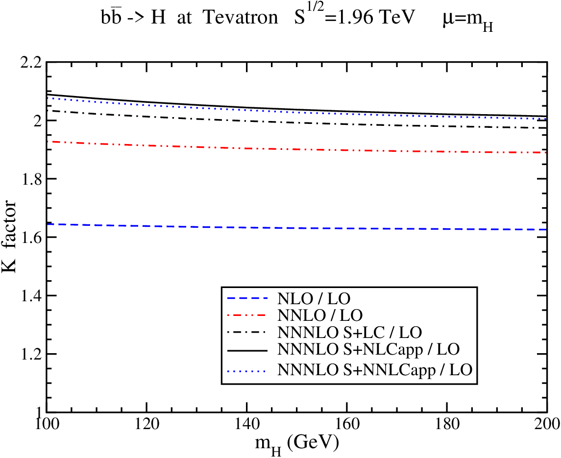
Figure 4: Left: The KK factors for b​b¯→Hb{\bar{b}}\rightarrow H at the Tevatron. Here μ=μF=μR=mH\mu=\mu_{F}=\mu_{R}=m_{H}. Right: The KK factors for b​b¯→Hb{\bar{b}}\rightarrow H at the LHC.

Figure 4 shows the KK factors, i.e. the ratios of the cross sections at various orders, for Higgs production via b​b¯→Hb{\bar{b}}\rightarrow H at the Tevatron (left-hand side) and the LHC (right-hand side), with μ=mH\mu=m_{H}. Here and in the rest of the figures NLO cross section means the Born term plus the 𝒪⁡(αs){\cal O}(\alpha_{s}) corrections, NNLO cross section means the Born term plus the 𝒪⁡(αs){\cal O}(\alpha_{s}) and 𝒪⁡(αs2){\cal O}(\alpha_{s}^{2}) corrections, and NNNLO cross section means the the Born term plus the 𝒪⁡(αs){\cal O}(\alpha_{s}) and 𝒪⁡(αs2){\cal O}(\alpha_{s}^{2}) and 𝒪⁡(αs3){\cal O}(\alpha_{s}^{3}) corrections. We note that we have used the same pdf for all curves because we are interested in the relative size of the terms in the perturbative expansion without the additional complications from different pdf. As the NLO / LO curve shows, the complete NLO corrections increase the LO result by around 60% at both the Tevatron and the LHC. The NNLO / LO curve shows that inclusion of the complete NNLO corrections futher increases the cross section by a substantial amount. The NNLO KK factor is around 1.9 at the Tevatron and 1.8 at the LHC. Finally, we include the approximate corrections (soft and collinear) at NNNLO. We note that the soft corrections are complete and we plot one curve with the soft and leading collinear (S+LC) terms, another curve with the soft and approximate next-to-leading collinear (S+NLCapp) terms, and a third with the soft and approximate next-to-next-to-leading collinear (S+NNLCapp) terms. We note that the difference between the S+LC and S+NLCapp curves is not very big, and between the S+NLCapp and S+NNLCapp curves it is quite small. Our investigation of the contributions of the soft and collinear terms at NLO and NNLO at both the Tevatron and the LHC gives us confidence that the NNNLO S+NNLCapp curves provide a good approximation of the complete NNNLO cross section. We note that the NNNLO S+NNLCapp KK factor is between 2.00 and 2.08 at the Tevatron and between 1.86 and 1.97 at the LHC for Higgs masses ranging between 100 and 200 GeV. In both cases the NNNLO corrections provide a significant enhancement over the NNLO result.
Refer to caption
Refer to caption
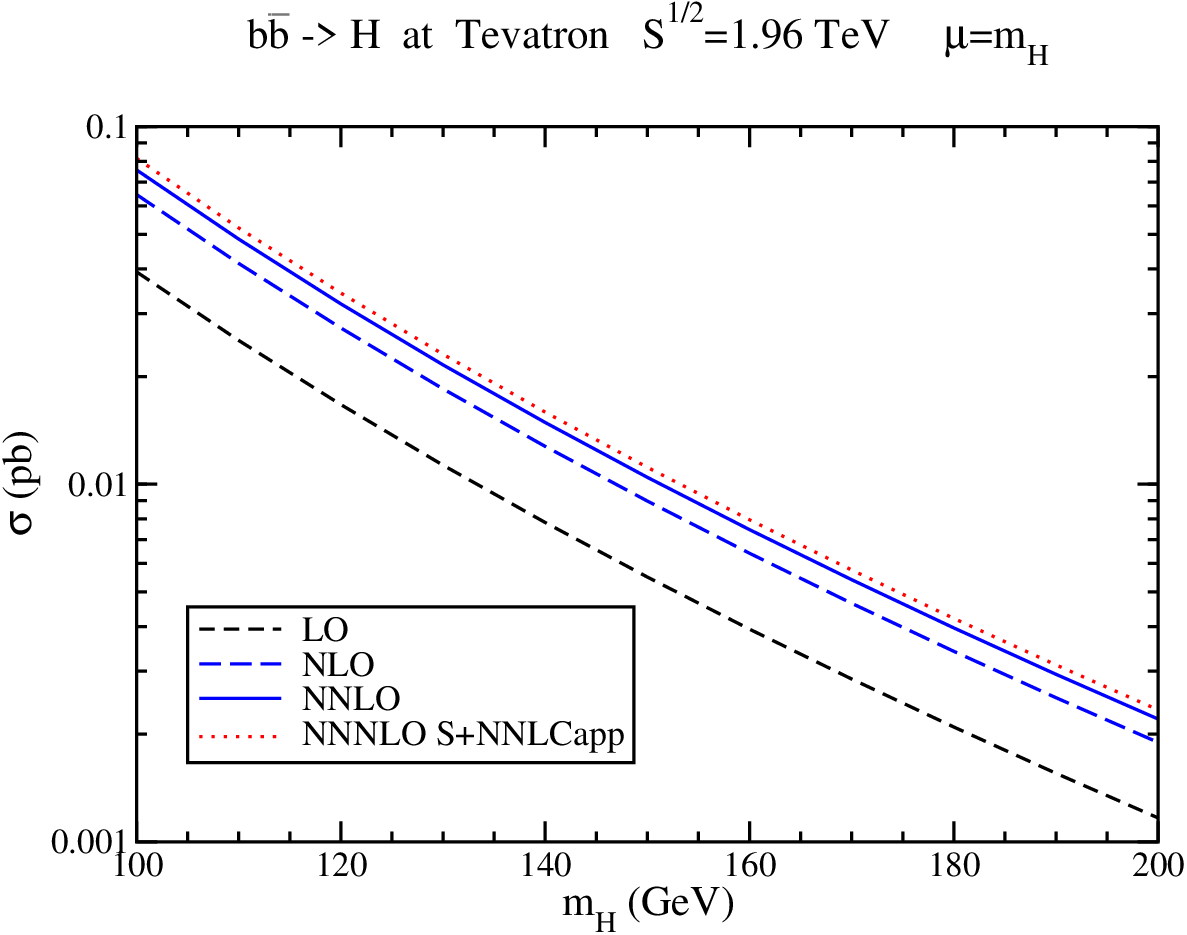
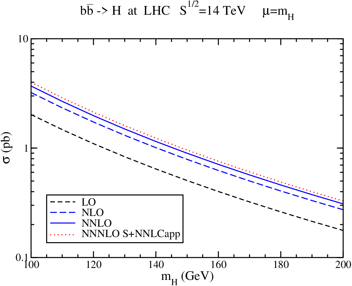
Figure 5: Left: The cross section for b​b¯→Hb{\bar{b}}\rightarrow H at the Tevatron with μ=μF=μR=mH\mu=\mu_{F}=\mu_{R}=m_{H}. Right: The cross section for b​b¯→Hb{\bar{b}}\rightarrow H at the LHC.

In Figure 5 we plot the cross sections for b​b¯→Hb{\bar{b}}\rightarrow H at the Tevatron (left-hand side) and the LHC (right-hand side). We show LO, NLO, NNLO, and NNNLO S+NNLCapp results for μ=mH\mu=m_{H}. We note that the NNLO SV+NLC(app) or NNLO SV+NNLC(app) results are indistinguishable from the exact NNLO curve on this plot. All five NNLO curves are on top of each other. This once again shows what we saw in more detail in figure 3, i.e. that our approximations including soft+virtual+next-to-(next-to)-leading collinear terms are excellent. Also, as expected from Figure 4, the NNNLO S+NLCapp curve is indistinguishable from NNNLO S+NNLCapp.

Refer to caption
Refer to caption
Figure 6: Left: The cross section for b​b¯→Hb{\bar{b}}\rightarrow H at the Tevatron with μ=μF=μR=mH/2,2​mH\mu=\mu_{F}=\mu_{R}=m_{H}/2,2m_{H}. Right: The cross section for b​b¯→Hb{\bar{b}}\rightarrow H at the LHC.

In Figure 6 we plot the cross sections for b​b¯→Hb{\bar{b}}\rightarrow H at the Tevatron (left-hand side) and the LHC (right-hand side) and show NNLO and NNNLO S+NNLCapp results for two choices of scale, μ=mH/2,2​mH\mu=m_{H}/2,2m_{H}. We note that if we plotted instead the NNNLO S+NLCapp results they would be indistinguishable from the NNNLO S+NNLCapp curves. From the figure we see that the NNNLO S+NNLCapp result has very similar scale variation to the NNLO result.

Finally, we calculate the uncertainty in the cross section from the parton distribution functions using the sets in [23] (pdf uncertainties for this process have also been studied in [25]). We find that the uncertainty is smaller at the LHC than at the Tevatron. For b​b¯→Hb{\bar{b}}\rightarrow H at the Tevatron we find that the pdf uncertainty varies from 3.1% for mH=100m_{H}=100 GeV to 5.6% for mH=150m_{H}=150 GeV to 8.0% for mH=200m_{H}=200 GeV. For b​b¯→Hb{\bar{b}}\rightarrow H at the LHC the pdf uncertainty varies from 2.0% for mH=100m_{H}=100 GeV to 1.6% for mH=150m_{H}=150 GeV to 1.3% for mH=200m_{H}=200 GeV. We thus see that the pfd uncertainty is non-negligible and can be of the same order of magnitude as the scale uncertainty, especially for large Higgs masses at the Tevatron.

5 Conclusions

We have studied Higgs production at the Tevatron and the LHC via the channel b​b¯→Hb{\bar{b}}\rightarrow H. We have calculated the complete soft corrections and the approximate next-to-next-to-leading collinear terms through NNNLO. We have shown that the inclusion of collinear corrections is essential in providing a good approximation to the complete cross section at NNLO. The soft and collinear NNNLO corrections provide significant enhancements to the cross section and must be taken into consideration for an improved theoretical prediction. The scale dependence of the cross section and the pdf uncertainties were also calculated. Analytical expressions for the soft and collinear corrections through NNNLO were also provided for g​g→Hgg\rightarrow H and the Drell-Yan process.

Acknowledgements

This work was supported by the National Science Foundation under Grant No. PHY 0555372. I would like to thank Jack Smith and Sasha Belyaev for useful conversations on Higgs production. I also thank V. Ravindran for detailed comparisons of our NNNLO calculations.

Appendix A: NNNLO soft and collinear corrections for Higgs and Drell-Yan processes: useful formulas

In this Appendix we first provide detailed expressions for the quantities that appear in the resummed cross section, Eq. (2.1). We then calculate a number of integrals for the soft and collinear corrections. Finally, we derive general formulas for the soft and collinear corrections for the processes under consideration in this paper.

A.1 Exponents in the resummed cross section

For the quantity AiA_{i} in the first exponent of Eq. (2.1) we use the expansion Ai​(αs)=Ai(1)​αs/π+Ai(2)​(αs/π)2+Ai(3)​(αs/π)3+⋯A_{i}(\alpha_{s})=A_{i}^{(1)}{\alpha_{s}/\pi}+A_{i}^{(2)}({\alpha_{s}/\pi})^{2}+A_{i}^{(3)}({\alpha_{s}/\pi})^{3}+\cdots. The results differ for quarks, i=qi=q, and gluons, i=gi=g. Here Aq(1)=CF=(Nc2−1)/(2​Nc)A_{q}^{(1)}=C_{F}=(N_{c}^{2}-1)/(2N_{c}) with Nc=3N_{c}=3 the number of colors, and Ag(1)=CA=NcA_{g}^{(1)}=C_{A}=N_{c}; Aq(2)=CF​K/2A_{q}^{(2)}=C_{F}K/2 with K=CA​(67/18−ζ2)−5​nf/9K=C_{A}(67/18-\zeta_{2})-5n_{f}/9 [26], where nfn_{f} is the number of light quark flavors (nf=5n_{f}=5 in our numerical results), and Ag(2)=CA​K/2A_{g}^{(2)}=C_{A}K/2; and Ai(3)A_{i}^{(3)} is given by [27]

Aq(3)\displaystyle A_{q}^{(3)} =\displaystyle= CF[CA2(24596−6736ζ2+1124ζ3+1120ζ22)+CFnf(−5596+ζ32)\displaystyle C_{F}\left[C_{A}^{2}\left(\frac{245}{96}-\frac{67}{36}\zeta_{2}+\frac{11}{24}\zeta_{3}+\frac{11}{20}\zeta_{2}^{2}\right)+C_{F}n_{f}\left(-\frac{55}{96}+\frac{\zeta_{3}}{2}\right)\right. (A.1)
+CAnf(−209432+518ζ2−712ζ3)−nf2108],\displaystyle\left.{}+C_{A}n_{f}\left(-\frac{209}{432}+\frac{5}{18}\zeta_{2}-\frac{7}{12}\zeta_{3}\right)-\frac{n_{f}^{2}}{108}\right]\,,
Ag(3)=CACF​Aq(3).A_{g}^{(3)}=\frac{C_{A}}{C_{F}}A_{q}^{(3)}\,. (A.2)

Here and below ζ2=π2/6\zeta_{2}=\pi^{2}/6, ζ3=1.2020569⋯\zeta_{3}=1.2020569\cdots, ζ4=π4/90\zeta_{4}=\pi^{4}/90, ζ5=1.0369278⋯\zeta_{5}=1.0369278\cdots.

Also νi=(αs/π)​νi(1)+(αs/π)2​νi(2)+(αs/π)3​νi(3)+⋯{\nu}_{i}=(\alpha_{s}/\pi){\nu}_{i}^{(1)}+(\alpha_{s}/\pi)^{2}{\nu}_{i}^{(2)}+(\alpha_{s}/\pi)^{3}{\nu}_{i}^{(3)}+\cdots, with νq(1)=CF{\nu}_{q}^{(1)}=C_{F} and νg(1)=CA{\nu}_{g}^{(1)}=C_{A}. It is convenient to lump together νi\nu_{i} with ΓS\Gamma_{S} as we discuss below.

In the second exponent of Eq. (2.1), γi/i\gamma_{i/i} is the moment-space anomalous dimension of the MS¯{\overline{\rm MS}} density ϕi/i\phi_{i/i} [28, 29]. We write

γi/i=γi(N)​ln⁡N+γi\gamma_{i/i}=\gamma_{i}^{(N)}\ln N+\gamma_{i} (A.3)

with

γq(N)\displaystyle\gamma_{q}^{(N)} =\displaystyle= −αsπ​CF​ln⁡N−(αsπ)2​CF​K2​ln⁡N+⋯\displaystyle-\frac{\alpha_{s}}{\pi}C_{F}\ln N-\left(\frac{\alpha_{s}}{\pi}\right)^{2}C_{F}\frac{K}{2}\ln N+\cdots
γg(N)\displaystyle\gamma_{g}^{(N)} =\displaystyle= −αsπ​CA​ln⁡N−(αsπ)2​CA​K2​ln⁡N+⋯,\displaystyle-\frac{\alpha_{s}}{\pi}C_{A}\ln N-\left(\frac{\alpha_{s}}{\pi}\right)^{2}C_{A}\frac{K}{2}\ln N+\cdots\,, (A.4)

and the parton anomalous dimensions

γi=(αs/π)​γi(1)+(αs/π)2​γi(2)+⋯\gamma_{i}=(\alpha_{s}/\pi)\gamma_{i}^{(1)}+(\alpha_{s}/\pi)^{2}\gamma_{i}^{(2)}+\cdots (A.5)

with γq(1)=3​CF/4\gamma_{q}^{(1)}=3C_{F}/4, γg(1)=β0/4\gamma_{g}^{(1)}=\beta_{0}/4,

γq(2)=CF2​(332−34​ζ2+32​ζ3)+CF​CA​(1796+1112​ζ2−34​ζ3)+nf​CF​(−148−ζ26),\gamma_{q}^{(2)}=C_{F}^{2}\left(\frac{3}{32}-\frac{3}{4}\zeta_{2}+\frac{3}{2}\zeta_{3}\right)+C_{F}C_{A}\left(\frac{17}{96}+\frac{11}{12}\zeta_{2}-\frac{3}{4}\zeta_{3}\right)+n_{f}C_{F}\left(-\frac{1}{48}-\frac{\zeta_{2}}{6}\right)\,, (A.6)

and

γg(2)=CA2​(23+34​ζ3)−nf​(CF8+CA6).\gamma_{g}^{(2)}=C_{A}^{2}\left(\frac{2}{3}+\frac{3}{4}\zeta_{3}\right)-n_{f}\left(\frac{C_{F}}{8}+\frac{C_{A}}{6}\right)\,. (A.7)

The β\beta function in the third exponent of Eq. (2.1) is given by

β(αs)≡12​αsd​αsd​ln⁡μ=μdlng/dμ=−β0αs/(4π)−β1αs2/(4π)2+⋯,\beta(\alpha_{s})\equiv\frac{1}{2\alpha_{s}}\frac{d\alpha_{s}}{d\ln\mu}=\mu\,d\ln g/d\mu=-\beta_{0}\alpha_{s}/(4\pi)-\beta_{1}\alpha_{s}^{2}/(4\pi)^{2}+\cdots\,, (A.8)

where g2=4​π​αsg^{2}=4\pi\alpha_{s}, with β0=(11​CA−2​nf)/3\beta_{0}=(11C_{A}-2n_{f})/3 and β1=34​CA2/3−2​nf​(CF+5​CA/3)\beta_{1}=34C_{A}^{2}/3-2n_{f}(C_{F}+5C_{A}/3) . Note that

αs​(μ)\displaystyle\alpha_{s}(\mu) =\displaystyle= αs(μR)[1−β04​παs(μR)ln(μ2μR2)+β0216​π2αs2(μR)ln2(μ2μR2)−β116​π2αs2(μR)ln(μ2μR2)\displaystyle\alpha_{s}(\mu_{R})\left[1-\frac{\beta_{0}}{4\pi}\alpha_{s}(\mu_{R})\ln\left(\frac{{\mu}^{2}}{\mu_{R}^{2}}\right)+\frac{\beta_{0}^{2}}{16\pi^{2}}\alpha_{s}^{2}(\mu_{R})\ln^{2}\left(\frac{{\mu}^{2}}{\mu_{R}^{2}}\right)-\frac{\beta_{1}}{16\pi^{2}}\alpha_{s}^{2}(\mu_{R})\ln\left(\frac{{\mu}^{2}}{\mu_{R}^{2}}\right)\right. (A.9)
+⋯].\displaystyle\hskip 56.9055pt\left.+\cdots\right]\,.

Also dαsd_{\alpha_{s}} is 0 for b​b¯→Hb{\bar{b}}\rightarrow H and q​q¯→Vq{\bar{q}}\rightarrow V and 2 for g​g→Hgg\rightarrow H.

The hard and soft functions can be expanded as H=αsdαs​H(0)+(αsdαs+1/π)​H(1)+(αsdαs+2/π2)​H(2)H=\alpha_{s}^{d_{\alpha_{s}}}H^{(0)}+(\alpha_{s}^{d_{\alpha_{s}}+1}/\pi)H^{(1)}+(\alpha_{s}^{d_{\alpha_{s}}+2}/\pi^{2})H^{(2)}+(αsdαs+3/π3)​H(3)+⋯+(\alpha_{s}^{d_{\alpha_{s}}+3}/\pi^{3})H^{(3)}+\cdots and S=S(0)+(αs/π)​S(1)+(αs/π)2​S(2)+(αs/π)3​S(3)+⋯S=S^{(0)}+(\alpha_{s}/\pi)S^{(1)}+(\alpha_{s}/\pi)^{2}S^{(2)}+(\alpha_{s}/\pi)^{3}S^{(3)}+\cdots. At lowest order, the Born cross section for the partonic process is σB=αsdαs​H(0)​S(0)\sigma^{B}=\alpha_{s}^{d_{\alpha_{s}}}H^{(0)}S^{(0)}.

The soft anomalous dimension is denoted by ΓS\Gamma_{S} and can be expanded as ΓS=(αs/π)​ΓS(1)\Gamma_{S}=(\alpha_{s}/\pi)\Gamma_{S}^{(1)} +(αs/π)2​ΓS(2)+(αs/π)3​ΓS(3)+⋯+(\alpha_{s}/\pi)^{2}\Gamma_{S}^{(2)}+(\alpha_{s}/\pi)^{3}\Gamma_{S}^{(3)}+\cdots. For the processes b​b¯→Hb{\bar{b}}\rightarrow H and q​q¯→Vq{\bar{q}}\rightarrow V, ΓS​q​q¯(1)=CF\Gamma^{(1)}_{S\,q{\bar{q}}}=C_{F}. For the process g​g→Hgg\rightarrow H, ΓS​g​g(1)=CA\Gamma^{(1)}_{S\,gg}=C_{A}. If we define G(n)=ΓS(n)−νi(n)G^{(n)}=\Gamma_{S}^{(n)}-\nu_{i}^{(n)} we can get explicit expressions through G(3)G^{(3)} [19, 30, 31]. We have Gq​q¯(1)=Gg​g(1)=0G_{q{\bar{q}}}^{(1)}=G_{gg}^{(1)}=0,

Gq​q¯(2)=CF​CA​(−10154+116​ζ2+74​ζ3)+13​CF​nf​(79−ζ2),G^{(2)}_{q\bar{q}}=C_{F}C_{A}\left(-\frac{101}{54}+\frac{11}{6}\zeta_{2}+\frac{7}{4}\zeta_{3}\right)+\frac{1}{3}C_{F}n_{f}\left(\frac{7}{9}-\zeta_{2}\right)\,, (A.10)
Gg​g(2)=CACF​Gq​q¯(2),G^{(2)}_{gg}=\frac{C_{A}}{C_{F}}G^{(2)}_{q\bar{q}}\,, (A.11)
Gq​q¯(3)\displaystyle G^{(3)}_{q\bar{q}} =\displaystyle= CF​CA2​(−29702946656+6139648​ζ2+2509216​ζ3−3​ζ5−187120​ζ22−1112​ζ2​ζ3)\displaystyle C_{F}C_{A}^{2}\left(-\frac{297029}{46656}+\frac{6139}{648}\zeta_{2}+\frac{2509}{216}\zeta_{3}-3\zeta_{5}-\frac{187}{120}\zeta_{2}^{2}-\frac{11}{12}\zeta_{2}\zeta_{3}\right) (A.12)
+CF​CA​nf​(3131323328−1837648​ζ2−15572​ζ3+2360​ζ22)\displaystyle{}+C_{F}C_{A}n_{f}\left(\frac{31313}{23328}-\frac{1837}{648}\zeta_{2}-\frac{155}{72}\zeta_{3}+\frac{23}{60}\zeta_{2}^{2}\right)
+CF2​nf​(17111728−ζ24−1936​ζ3−ζ2210)+CF​nf2​(−29729+527​ζ2+554​ζ3),\displaystyle{}+C_{F}^{2}n_{f}\left(\frac{1711}{1728}-\frac{\zeta_{2}}{4}-\frac{19}{36}\zeta_{3}-\frac{\zeta_{2}^{2}}{10}\right)+C_{F}n_{f}^{2}\left(-\frac{29}{729}+\frac{5}{27}\zeta_{2}+\frac{5}{54}\zeta_{3}\right)\,,
Gg​g(3)=CACF​Gq​q¯(3).G^{(3)}_{gg}=\frac{C_{A}}{C_{F}}G^{(3)}_{q\bar{q}}\,. (A.13)

A.2 Useful integrals

In the resummed cross section we encounter certain integrals that need to be evaluated. They are of the form

In​(N)=∫01d​z​zN−1​[lnn⁡(1−z)1−z]+.I_{n}(N)=\int_{0}^{1}dz\,z^{N-1}\left[\frac{\ln^{n}(1-z)}{1-z}\right]_{+}\,. (A.14)

The expressions for InI_{n} have been presented up to n=7n=7 in [21] and including 1/N1/N terms up to n=3n=3 in [12]. Here we extend these results by including 1/N1/N terms up to n=5n=5, which are needed for NNNLO expansions:

I0​(N)\displaystyle I_{0}(N) =\displaystyle= −ln⁡N~+12​N\displaystyle-\ln{\tilde{N}}+\frac{1}{2N}
I1​(N)\displaystyle I_{1}(N) =\displaystyle= 12​ln2​N~+ζ22−(ln⁡N~+1)​12​N\displaystyle\frac{1}{2}\ln^{2}{\tilde{N}}+\frac{\zeta_{2}}{2}-(\ln{\tilde{N}}+1)\frac{1}{2N}
I2​(N)\displaystyle I_{2}(N) =\displaystyle= −13​ln3​N~−ζ2​ln⁡N~−23​ζ3+(12​ln2​N~+ζ22+ln⁡N~)​1N\displaystyle-\frac{1}{3}\ln^{3}{\tilde{N}}-\zeta_{2}\ln{\tilde{N}}-\frac{2}{3}\zeta_{3}+\left(\frac{1}{2}\ln^{2}{\tilde{N}}+\frac{\zeta_{2}}{2}+\ln{\tilde{N}}\right)\frac{1}{N}
I3​(N)\displaystyle I_{3}(N) =\displaystyle= 14​ln4​N~+32​ζ2​ln2​N~+2​ζ3​ln⁡N~+32​ζ4+34​ζ22\displaystyle\frac{1}{4}\ln^{4}{\tilde{N}}+\frac{3}{2}\zeta_{2}\ln^{2}{\tilde{N}}+2\zeta_{3}\ln{\tilde{N}}+\frac{3}{2}\zeta_{4}+\frac{3}{4}\zeta_{2}^{2}
+(−12​ln3​N~−32​ζ2​ln⁡N~−ζ3−32​ln2​N~−32​ζ2)​1N\displaystyle{}+\left(-\frac{1}{2}\ln^{3}{\tilde{N}}-\frac{3}{2}\zeta_{2}\ln{\tilde{N}}-\zeta_{3}-\frac{3}{2}\ln^{2}{\tilde{N}}-\frac{3}{2}\zeta_{2}\right)\frac{1}{N}
I4​(N)\displaystyle I_{4}(N) =\displaystyle= −15​ln5​N~−2​ζ2​ln3​N~−4​ζ3​ln2​N~−3​(ζ22+2​ζ4)​ln⁡N~−4​(ζ2​ζ3+65​ζ5)\displaystyle-\frac{1}{5}\ln^{5}{\tilde{N}}-2\zeta_{2}\ln^{3}{\tilde{N}}-4\zeta_{3}\ln^{2}{\tilde{N}}-3(\zeta_{2}^{2}+2\zeta_{4})\ln{\tilde{N}}-4\left(\zeta_{2}\zeta_{3}+\frac{6}{5}\zeta_{5}\right)
+(12​ln4​N~+3​ζ2​ln2​N~+4​ζ3​ln​N~+32​ζ22+3​ζ4+2​ln3​N~+6​ζ2​ln​N~+4​ζ3)​1N\displaystyle{}+\left(\frac{1}{2}\ln^{4}{\tilde{N}}+3\zeta_{2}\ln^{2}{\tilde{N}}+4\zeta_{3}\ln{\tilde{N}}+\frac{3}{2}\zeta_{2}^{2}+3\zeta_{4}+2\ln^{3}{\tilde{N}}+6\zeta_{2}\ln{\tilde{N}}+4\zeta_{3}\right)\frac{1}{N}
I5​(N)\displaystyle I_{5}(N) =\displaystyle= 16​ln6​N~+52​ζ2​ln4​N~+203​ζ3​ln3​N~+152​(ζ22+2​ζ4)​ln2​N~\displaystyle\frac{1}{6}\ln^{6}{\tilde{N}}+\frac{5}{2}\zeta_{2}\ln^{4}{\tilde{N}}+\frac{20}{3}\zeta_{3}\ln^{3}{\tilde{N}}+\frac{15}{2}(\zeta_{2}^{2}+2\zeta_{4})\ln^{2}{\tilde{N}} (A.15)
+4​(5​ζ2​ζ3+6​ζ5)​ln⁡N~+5​(ζ232+43​ζ32+3​ζ2​ζ4+4​ζ6)\displaystyle{}+4(5\zeta_{2}\zeta_{3}+6\zeta_{5})\ln{\tilde{N}}+5\left(\frac{\zeta_{2}^{3}}{2}+\frac{4}{3}\zeta_{3}^{2}+3\zeta_{2}\zeta_{4}+4\zeta_{6}\right)
+(−12​ln5​N~−5​ζ2​ln3​N~−10​ζ3​ln2​N~−152​(ζ22+2​ζ4)​ln⁡N~−10​(ζ2​ζ3+65​ζ5)CLOSE\displaystyle{}+\left(-\frac{1}{2}\ln^{5}{\tilde{N}}-5\zeta_{2}\ln^{3}{\tilde{N}}-10\zeta_{3}\ln^{2}{\tilde{N}}-\frac{15}{2}(\zeta_{2}^{2}+2\zeta_{4})\ln{\tilde{N}}-10\left(\zeta_{2}\zeta_{3}+\frac{6}{5}\zeta_{5}\right)\right.
OPEN−52​ln4​N~−15​ζ2​ln2​N~−20​ζ3​ln⁡N~−152​ζ22−15​ζ4)​1N.\displaystyle\quad\left.{}-\frac{5}{2}\ln^{4}{\tilde{N}}-15\zeta_{2}\ln^{2}{\tilde{N}}-20\zeta_{3}\ln{\tilde{N}}-\frac{15}{2}\zeta_{2}^{2}-15\zeta_{4}\right)\frac{1}{N}\,.

We also encounter integrals of the form

Jn​(N)=∫01d​z​zN−1​lnn⁡(1−z).J_{n}(N)=\int_{0}^{1}dz\,z^{N-1}\ln^{n}(1-z)\,. (A.16)

The expressions for JnJ_{n} have been presented up to n=3n=3 in [12]. Here we extend these results up to n=5n=5, which are needed for NNNLO expansions:

J0​(N)\displaystyle J_{0}(N) =\displaystyle= 1NJ1​(N)=−ln⁡N~NJ2​(N)=ln2⁡N~N+ζ2N\displaystyle\frac{1}{N}\quad\quad\quad J_{1}(N)=-\frac{\ln{\tilde{N}}}{N}\quad\quad\quad J_{2}(N)=\frac{\ln^{2}{\tilde{N}}}{N}+\frac{\zeta_{2}}{N}
J3​(N)\displaystyle J_{3}(N) =\displaystyle= −ln3⁡N~N−3​ζ2​ln⁡N~N−2​ζ3N\displaystyle-\frac{\ln^{3}{\tilde{N}}}{N}-3\zeta_{2}\frac{\ln{\tilde{N}}}{N}-2\frac{\zeta_{3}}{N}
J4​(N)\displaystyle J_{4}(N) =\displaystyle= ln4⁡N~N+6​ζ2​ln2⁡N~N+8​ζ3​ln⁡N~N+(3​ζ22+6​ζ4)​1N\displaystyle\frac{\ln^{4}{\tilde{N}}}{N}+6\zeta_{2}\frac{\ln^{2}{\tilde{N}}}{N}+8\zeta_{3}\frac{\ln{\tilde{N}}}{N}+(3\zeta_{2}^{2}+6\zeta_{4})\frac{1}{N}
J5​(N)\displaystyle J_{5}(N) =\displaystyle= −ln5⁡N~N−10​ζ2​ln3⁡N~N−20​ζ3​ln2⁡N~N−15​(ζ22+2​ζ4)​ln⁡N~N−20​(ζ2​ζ3+65​ζ5)​1N.\displaystyle-\frac{\ln^{5}{\tilde{N}}}{N}-10\zeta_{2}\frac{\ln^{3}{\tilde{N}}}{N}-20\zeta_{3}\frac{\ln^{2}{\tilde{N}}}{N}-15(\zeta_{2}^{2}+2\zeta_{4})\frac{\ln{\tilde{N}}}{N}-20\left(\zeta_{2}\zeta_{3}+\frac{6}{5}\zeta_{5}\right)\frac{1}{N}\,.

A.3 General formulas for soft and collinear corrections

Below, we write general expressions for the soft and collinear corrections at NLO, NNLO, and NNNLO for the processes under study. Detailed results are provided in Section 3 for b​b¯→Hb{\bar{b}}\rightarrow H, in Appendix B for the Drell-Yan process, and in Appendix C for g​g→Hgg\rightarrow H. We note that for processes involving a quark running mass, such as b​b¯→Hb{\bar{b}}\rightarrow H, the expressions below are valid for the running mass at scale MM. If the mass is evaluated at scale μR\mu_{R} (as in Section 3) we have to include additional terms as discussed at the end of this appendix.

The NLO soft and virtual corrections are given by

σ^(1)​S​V=FB​αs​(μR2)π​{c3​𝒟1​(z)+c2​𝒟0​(z)+c1​δ​(1−z)}{\hat{\sigma}}^{(1)\,SV}=F^{B}\frac{\alpha_{s}(\mu_{R}^{2})}{\pi}\left\{c_{3}\,{\cal D}_{1}(z)+c_{2}\,{\cal D}_{0}(z)+c_{1}\,\delta(1-z)\right\} (A.18)

where FBF^{B} is the Born term and

Dl​(z)=[lnl⁡(1−z)1−z]+D_{l}(z)=\left[\frac{\ln^{l}(1-z)}{1-z}\right]_{+} (A.19)

with z=M2/sz=M^{2}/s. If we define CiC_{i} to denote CFC_{F} for quarks and CAC_{A} for gluons then the coefficients are given by

c3=4​Cic_{3}=4C_{i} (A.20)
c2=−2​Ci​ln⁡(μF2M2)c_{2}=-2C_{i}\ln\left(\frac{\mu_{F}^{2}}{M^{2}}\right) (A.21)
c1=T1+c1μc_{1}=T_{1}+c_{1}^{\mu} (A.22)

with

c1μ=−2​γi(1)​ln⁡(μF2M2)+dαs​β04​ln⁡(μR2M2),c_{1}^{\mu}=-2\gamma_{i}^{(1)}\ln\left(\frac{\mu_{F}^{2}}{M^{2}}\right)+d_{\alpha_{s}}\frac{\beta_{0}}{4}\ln\left(\frac{\mu_{R}^{2}}{M^{2}}\right)\,, (A.23)

and T1T_{1} the scale-independent virtual corrections for each process. We note that c2c_{2} only involves the scale dependence. This simplifies the structure of the results at higher orders.

The NLO collinear corrections are given by

σ^(1)​C=FB​αs​(μR2)π​{c3c​ln⁡(1−z)+c2c}{\hat{\sigma}}^{(1)\,C}=F^{B}\frac{\alpha_{s}(\mu_{R}^{2})}{\pi}\left\{c_{3}^{c}\,\ln(1-z)+c_{2}^{c}\right\} (A.24)

where c3c=−4​Ci​κic_{3}^{c}=-4C_{i}\kappa_{i} and c2c=2​Ci​κi​ln⁡(μF2/M2)+2​Cic_{2}^{c}=2C_{i}\kappa_{i}\ln(\mu_{F}^{2}/M^{2})+2C_{i}, where κq=1\kappa_{q}=1 and κg=2\kappa_{g}=2.

The NNLO soft and virtual corrections are given by

σ^(2)​S​V\displaystyle{\hat{\sigma}}^{(2)\,SV} =\displaystyle= FBαs2​(μR2)π2{12c32𝒟3(z)+[32c3c2−β04c3]𝒟2(z)\displaystyle F^{B}\frac{\alpha_{s}^{2}(\mu_{R}^{2})}{\pi^{2}}\left\{\frac{1}{2}c_{3}^{2}\,{\cal D}_{3}(z)+\left[\frac{3}{2}c_{3}\,c_{2}-\frac{\beta_{0}}{4}c_{3}\right]\,{\cal D}_{2}(z)\right. (A.25)
+[c3​c1+c22−ζ2​c32+β04​c3​ln⁡(μR2M2)+c32​K]​𝒟1​(z)\displaystyle{}+\left[c_{3}\,c_{1}+c_{2}^{2}-\zeta_{2}\,c_{3}^{2}+\frac{\beta_{0}}{4}c_{3}\ln\left(\frac{\mu_{R}^{2}}{M^{2}}\right)+\frac{c_{3}}{2}K\right]\,{\cal D}_{1}(z)
+[c2c1−ζ2c3c2+ζ3c32+2Gi​i(2)+β04c2ln(μR2M2)\displaystyle{}+\left[c_{2}c_{1}-\zeta_{2}\,c_{3}\,c_{2}+\zeta_{3}\,c_{3}^{2}+2G^{(2)}_{ii}+\frac{\beta_{0}}{4}c_{2}\ln\left(\frac{\mu_{R}^{2}}{M^{2}}\right)\right.
+Ciβ04ln2(μF2M2)−CiKln(μF2M2)]𝒟0(z)\displaystyle\quad\left.{}+C_{i}\frac{\beta_{0}}{4}\ln^{2}\left(\frac{\mu_{F}^{2}}{M^{2}}\right)-C_{i}K\ln\left(\frac{\mu_{F}^{2}}{M^{2}}\right)\right]\,{\cal D}_{0}(z)
+[V(2)+12(c12−T12)−ζ22c22+ζ3c3c2+β04c1ln(μR2M2)−2γi(2)ln(μF2M2)\displaystyle{}+\left[V^{(2)}+\frac{1}{2}(c_{1}^{2}-T_{1}^{2})-\frac{\zeta_{2}}{2}c_{2}^{2}+\zeta_{3}c_{3}c_{2}+\frac{\beta_{0}}{4}c_{1}\ln\left(\frac{\mu_{R}^{2}}{M^{2}}\right)-2{\gamma}_{i}^{(2)}\ln\left(\frac{\mu_{F}^{2}}{M^{2}}\right)\right.
+β04γi(1)ln2(μF2M2)−dαs32β02ln2(μR2M2)+dαs16β1ln(μR2M2)]δ(1−z)}\displaystyle\quad\left.\left.{}+\frac{\beta_{0}}{4}{\gamma}_{i}^{(1)}\ln^{2}\left(\frac{\mu_{F}^{2}}{M^{2}}\right)-\frac{d_{\alpha_{s}}}{32}\beta_{0}^{2}\ln^{2}\left(\frac{\mu_{R}^{2}}{M^{2}}\right)+\frac{d_{\alpha_{s}}}{16}\beta_{1}\ln\left(\frac{\mu_{R}^{2}}{M^{2}}\right)\right]\delta(1-z)\right\}

where V(2)V^{(2)} denotes the two-loop virtual scale-independent terms for each process, which cannot be derived from resummation.

The NNLO (approximate) collinear corrections are given by

σ^(2)​C\displaystyle{\hat{\sigma}}^{(2)\,C} =\displaystyle= FBαs2​(μR2)π2{12c3c3cln3(1−z)+[12c3c2c+c2c3c+12c32−β04c3c]ln2(1−z)\displaystyle F^{B}\frac{\alpha_{s}^{2}(\mu_{R}^{2})}{\pi^{2}}\left\{\frac{1}{2}c_{3}c_{3}^{c}\,\ln^{3}(1-z)+\left[\frac{1}{2}c_{3}c_{2}^{c}+c_{2}c_{3}^{c}+\frac{1}{2}c_{3}^{2}-\frac{\beta_{0}}{4}c_{3}^{c}\right]\ln^{2}(1-z)\right. (A.26)
+[c1​c3c+c2​c2c−ζ2​c3​c3c+c3​c2+β04​c3c​ln⁡(μR2M2)+12​c3c​K−β02​T2c]​ln⁡(1−z)\displaystyle{}+\left[c_{1}c_{3}^{c}+c_{2}c_{2}^{c}-\zeta_{2}c_{3}c_{3}^{c}+c_{3}c_{2}+\frac{\beta_{0}}{4}c_{3}^{c}\ln\left(\frac{\mu_{R}^{2}}{M^{2}}\right)+\frac{1}{2}c_{3}^{c}K-\frac{\beta_{0}}{2}T_{2}^{c}\right]\ln(1-z)
+const.}\displaystyle\left.{}+{\rm const.}\right\}

where T2c=2​CiT_{2}^{c}=2C_{i} denotes the scale-independent part of c2cc_{2}^{c}. Note that only the leading terms are complete. However, the ln2⁡(1−z)\ln^{2}(1-z) and ln⁡(1−z)\ln(1-z) are nearly complete as discussed elsewhere in the paper. We do not calculate the constants other than the scale-dependent terms as described elsewhere in the paper.

The NNNLO soft-gluon corrections are given by

σ^(3)​S\displaystyle{\hat{\sigma}}^{(3)\,S} =\displaystyle= FBαs3​(μR2)π3{18c33𝒟5(z)+524(3c32c2−β0c32)𝒟4(z)\displaystyle F^{B}\frac{\alpha_{s}^{3}(\mu_{R}^{2})}{\pi^{3}}\;\left\{\frac{1}{8}c_{3}^{3}\;{\cal D}_{5}(z)+\frac{5}{24}\left(3c_{3}^{2}c_{2}-\beta_{0}c_{3}^{2}\right)\;{\cal D}_{4}(z)\right. (A.27)
+[c3​c22+12​c32​c1−ζ2​c33−β03​c3​c2+β0212​c3+K2​c32+β04​c32​ln⁡(μR2M2)]​𝒟3​(z)\displaystyle\hskip-42.67912pt{}+\left[c_{3}c_{2}^{2}+\frac{1}{2}c_{3}^{2}c_{1}-\zeta_{2}c_{3}^{3}-\frac{\beta_{0}}{3}c_{3}c_{2}+\frac{\beta_{0}^{2}}{12}c_{3}+\frac{K}{2}c_{3}^{2}+\frac{\beta_{0}}{4}c_{3}^{2}\ln\left(\frac{\mu_{R}^{2}}{M^{2}}\right)\right]\;{\cal D}_{3}(z)
+[32c3c2c1+12c23−3ζ2c32c2+52ζ3c33−β04c3c1+34β0ζ2c32+34Kc3c2−β04Kc3−β14Ci\displaystyle\hskip-42.67912pt{}+\left[\frac{3}{2}c_{3}c_{2}\,c_{1}+\frac{1}{2}c_{2}^{3}-3\zeta_{2}c_{3}^{2}c_{2}+\frac{5}{2}\zeta_{3}c_{3}^{3}-\frac{\beta_{0}}{4}c_{3}c_{1}+\frac{3}{4}\beta_{0}\zeta_{2}c_{3}^{2}+\frac{3}{4}Kc_{3}c_{2}-\frac{\beta_{0}}{4}Kc_{3}-\frac{\beta_{1}}{4}C_{i}\right.
+3c3Gi​i(2)+38Ciβ0c3ln2(μF2M2)−32CiKc3ln(μF2M2)+(34β0c3c2−β028c3)ln(μR2M2)]𝒟2(z)\displaystyle\hskip-28.45274pt\left.{}+3c_{3}G^{(2)}_{ii}+\frac{3}{8}C_{i}\beta_{0}c_{3}\ln^{2}\left(\frac{\mu_{F}^{2}}{M^{2}}\right)-\frac{3}{2}C_{i}Kc_{3}\ln\left(\frac{\mu_{F}^{2}}{M^{2}}\right)+\left(\frac{3}{4}\beta_{0}c_{3}c_{2}-\frac{\beta_{0}^{2}}{8}c_{3}\right)\ln\left(\frac{\mu_{R}^{2}}{M^{2}}\right)\right]\;{\cal D}_{2}(z)
+[c32(c12−T12)+c22c1−ζ2c32c1−52ζ2c3c22+5ζ3c32c2−3ζ4c33+ζ22c33+β02ζ2c3c2−32β0ζ3c32\displaystyle\hskip-42.67912pt{}+\left[\frac{c_{3}}{2}(c_{1}^{2}-T_{1}^{2})+c_{2}^{2}c_{1}-\zeta_{2}c_{3}^{2}c_{1}-\frac{5}{2}\zeta_{2}c_{3}c_{2}^{2}+5\zeta_{3}c_{3}^{2}c_{2}-3\zeta_{4}c_{3}^{3}+\zeta_{2}^{2}c_{3}^{3}+\frac{\beta_{0}}{2}\zeta_{2}c_{3}c_{2}-\frac{3}{2}\beta_{0}\zeta_{3}c_{3}^{2}\right.
+K2​c3​c1+Ci​ζ2​K​c3−54​ζ2​K​c32+(4​c2−2​β0)​Gi​i(2)+c3​V(2)+4​Ai(3)+β04​(c3​γi(1)+2​Ci​c2)​ln2⁡(μF2M2)\displaystyle\hskip-28.45274pt{}+\frac{K}{2}c_{3}c_{1}+C_{i}\zeta_{2}Kc_{3}-\frac{5}{4}\zeta_{2}Kc_{3}^{2}+(4c_{2}-2\beta_{0})G^{(2)}_{ii}+c_{3}V^{(2)}+4A_{i}^{(3)}+\frac{\beta_{0}}{4}\left(c_{3}\gamma_{i}^{(1)}+2C_{i}c_{2}\right)\ln^{2}\left(\frac{\mu_{F}^{2}}{M^{2}}\right)
−2​(c3​γi(2)+Ci​K​c2)​ln⁡(μF2M2)−β022​Ci​ln⁡(μF2M2)​ln⁡(μR2M2)+β0232​(8​Ci−c3​dαs)​ln2⁡(μR2M2)\displaystyle\hskip-28.45274pt{}-2\left(c_{3}\gamma_{i}^{(2)}+C_{i}Kc_{2}\right)\ln\left(\frac{\mu_{F}^{2}}{M^{2}}\right)-\frac{\beta_{0}^{2}}{2}C_{i}\ln\left(\frac{\mu_{F}^{2}}{M^{2}}\right)\ln\left(\frac{\mu_{R}^{2}}{M^{2}}\right)+\frac{\beta_{0}^{2}}{32}\left(8C_{i}-c_{3}d_{\alpha_{s}}\right)\ln^{2}\left(\frac{\mu_{R}^{2}}{M^{2}}\right)
+(β02(c3c1+c22−ζ2c32+2CiK)−β024c2+β116(4Ci+c3dαs))ln(μR2M2)]𝒟1(z)\displaystyle\hskip-28.45274pt\left.{}+\left(\frac{\beta_{0}}{2}(c_{3}c_{1}+c_{2}^{2}-\zeta_{2}c_{3}^{2}+2C_{i}K)-\frac{\beta_{0}^{2}}{4}c_{2}+\frac{\beta_{1}}{16}(4C_{i}+c_{3}d_{\alpha_{s}})\right)\ln\left(\frac{\mu_{R}^{2}}{M^{2}}\right)\right]\;{\cal D}_{1}(z)
+[c22(c12−T12)−ζ2c3c2c1−ζ22c23+ζ3c32c1+2ζ3c3c22−3ζ4c32c2+3ζ5c33+ζ22c32c2−2ζ2ζ3c33+Ciζ2Kc2\displaystyle\hskip-42.67912pt{}+\left[\frac{c_{2}}{2}(c_{1}^{2}-T_{1}^{2})-\zeta_{2}c_{3}c_{2}c_{1}-\frac{\zeta_{2}}{2}c_{2}^{3}+\zeta_{3}c_{3}^{2}c_{1}+2\zeta_{3}c_{3}c_{2}^{2}-3\zeta_{4}c_{3}^{2}c_{2}+3\zeta_{5}c_{3}^{3}+\zeta_{2}^{2}c_{3}^{2}c_{2}-2\zeta_{2}\zeta_{3}c_{3}^{3}+C_{i}\zeta_{2}Kc_{2}\right.
−34​ζ2​K​c3​c2+ζ3​K​c32−β02​ζ3​c3​c2+54​β0​ζ4​c32−β04​c32​ζ22+2​(c1−ζ2​c3)​Gi​i(2)+c2​V(2)+2​Gi​i(3)\displaystyle\hskip-28.45274pt{}-\frac{3}{4}\zeta_{2}Kc_{3}c_{2}+\zeta_{3}Kc_{3}^{2}-\frac{\beta_{0}}{2}\zeta_{3}c_{3}c_{2}+\frac{5}{4}\beta_{0}\zeta_{4}c_{3}^{2}-\frac{\beta_{0}}{4}c_{3}^{2}\zeta_{2}^{2}+2(c_{1}-\zeta_{2}c_{3})G^{(2)}_{ii}+c_{2}V^{(2)}+2G^{(3)}_{ii}
−β0224​Ci​ln3⁡(μF2M2)+(β04​(Ci​c1−Ci​ζ2​c3+Ci​K+c2​γi(1))+β116​Ci)​ln2⁡(μF2M2)\displaystyle\hskip-28.45274pt{}-\frac{\beta_{0}^{2}}{24}C_{i}\ln^{3}\left(\frac{\mu_{F}^{2}}{M^{2}}\right)+\left(\frac{\beta_{0}}{4}(C_{i}c_{1}-C_{i}\zeta_{2}c_{3}+C_{i}K+c_{2}\gamma_{i}^{(1)})+\frac{\beta_{1}}{16}C_{i}\right)\ln^{2}\left(\frac{\mu_{F}^{2}}{M^{2}}\right)
+β028​Ci​ln2⁡(μF2M2)​ln⁡(μR2M2)−β028​Ci​ln⁡(μF2M2)​ln2⁡(μR2M2)−dαs32​c2​β02​ln2⁡(μR2M2)\displaystyle\hskip-28.45274pt{}+\frac{\beta_{0}^{2}}{8}C_{i}\ln^{2}\left(\frac{\mu_{F}^{2}}{M^{2}}\right)\ln\left(\frac{\mu_{R}^{2}}{M^{2}}\right)-\frac{\beta_{0}^{2}}{8}C_{i}\ln\left(\frac{\mu_{F}^{2}}{M^{2}}\right)\ln^{2}\left(\frac{\mu_{R}^{2}}{M^{2}}\right)-\frac{d_{\alpha_{s}}}{32}c_{2}\beta_{0}^{2}\ln^{2}\left(\frac{\mu_{R}^{2}}{M^{2}}\right)
−Ci8​(4​β0​K+β1)​ln⁡(μF2M2)​ln⁡(μR2M2)+(−Ci​K​c1+Ci​ζ2​K​c3−2​c2​γi(2)−2​Ai(3))​ln⁡(μF2M2)\displaystyle\hskip-28.45274pt{}-\frac{C_{i}}{8}(4\beta_{0}K+\beta_{1})\ln\left(\frac{\mu_{F}^{2}}{M^{2}}\right)\ln\left(\frac{\mu_{R}^{2}}{M^{2}}\right)+\left(-C_{i}Kc_{1}+C_{i}\zeta_{2}Kc_{3}-2c_{2}\gamma_{i}^{(2)}-2A_{i}^{(3)}\right)\ln\left(\frac{\mu_{F}^{2}}{M^{2}}\right)
+(β02(c2c1−ζ2c3c2+ζ3c32+2Gi​i(2))+dαs16c2β1)ln(μR2M2)]𝒟0(z)}.\displaystyle\hskip-28.45274pt\left.\left.{}+\left(\frac{\beta_{0}}{2}(c_{2}c_{1}-\zeta_{2}c_{3}c_{2}+\zeta_{3}c_{3}^{2}+2G^{(2)}_{ii})+\frac{d_{\alpha_{s}}}{16}c_{2}\beta_{1}\right)\ln\left(\frac{\mu_{R}^{2}}{M^{2}}\right)\right]\;{\cal D}_{0}(z)\right\}\,.

The NNNLO (approximate) collinear corrections are given by

σ^(3)​C\displaystyle{\hat{\sigma}}^{(3)\,C} =\displaystyle= FBαs3​(μR2)π3{18c32c3cln5(1−z)+[18c32c2c+12c3c2c3c−c3316−524β0c3c3c]ln4(1−z)\displaystyle F^{B}\frac{\alpha_{s}^{3}(\mu_{R}^{2})}{\pi^{3}}\left\{\frac{1}{8}c_{3}^{2}c_{3}^{c}\,\ln^{5}(1-z)+\left[\frac{1}{8}c_{3}^{2}c_{2}^{c}+\frac{1}{2}c_{3}c_{2}c_{3}^{c}-\frac{c_{3}^{3}}{16}-\frac{5}{24}\beta_{0}c_{3}c_{3}^{c}\right]\ln^{4}(1-z)\right. (A.28)
+[12c3c1c3c+12c22c3c+12c3c2c2c−ζ2c32c3c−14c32c2+β0212c3c−β04c32−β04c2c3c−β012c3c2c\displaystyle{}+\left[\frac{1}{2}c_{3}c_{1}c_{3}^{c}+\frac{1}{2}c_{2}^{2}c_{3}^{c}+\frac{1}{2}c_{3}c_{2}c_{2}^{c}-\zeta_{2}c_{3}^{2}c_{3}^{c}-\frac{1}{4}c_{3}^{2}c_{2}+\frac{\beta_{0}^{2}}{12}c_{3}^{c}-\frac{\beta_{0}}{4}c_{3}^{2}-\frac{\beta_{0}}{4}c_{2}c_{3}^{c}-\frac{\beta_{0}}{12}c_{3}c_{2}^{c}\right.
−β04c3T2c+12c3c3cK+β04c3c3cln(μR2M2)]ln3(1−z)+𝒪(ln2(1−z))}.\displaystyle\left.\left.{}-\frac{\beta_{0}}{4}c_{3}T_{2}^{c}+\frac{1}{2}c_{3}c_{3}^{c}K+\frac{\beta_{0}}{4}c_{3}c_{3}^{c}\ln\left(\frac{\mu_{R}^{2}}{M^{2}}\right)\right]\ln^{3}(1-z)+{\cal O}(\ln^{2}(1-z))\right\}\,.

Note that only the leading terms are complete. However, the ln4⁡(1−z)\ln^{4}(1-z) and ln3⁡(1−z)\ln^{3}(1-z) are expected to be nearly complete as discussed elsewhere in the paper. We do not calculate ln2⁡(1−z)\ln^{2}(1-z) or lower terms other than some scale-dependent terms as described elsewhere in the paper.

In the calculation of b​b¯→Hb{\bar{b}}\rightarrow H we also have to consider the renormalization scale logarithms from the MS¯\overline{\rm MS} bottom quark running mass, mbm_{b}. Since μ2​d​mb/d​μ2=−γm​mb\mu^{2}dm_{b}/d\mu^{2}=-\gamma_{m}m_{b} with γm\gamma_{m} the mass anomalous dimension [32]

γm=αsπ​34​CF+αs2π2​(332​CF2+9796​CF​CA−548​nf​CF)+𝒪⁡(αs3)\gamma_{m}=\frac{\alpha_{s}}{\pi}\frac{3}{4}C_{F}+\frac{\alpha_{s}^{2}}{\pi^{2}}\left(\frac{3}{32}C_{F}^{2}+\frac{97}{96}C_{F}C_{A}-\frac{5}{48}n_{f}C_{F}\right)+{\cal O}(\alpha_{s}^{3}) (A.29)

we have

mb2​(mH2)\displaystyle m_{b}^{2}(m_{H}^{2}) =\displaystyle= mb2(μR2){1+αs​(μR2)π32CFln(μR2mH2)+αs2​(μR2)π2[(98CF2−3​β016CF)ln2(μR2mH2)\displaystyle m_{b}^{2}(\mu_{R}^{2})\left\{1+\frac{\alpha_{s}(\mu_{R}^{2})}{\pi}\frac{3}{2}C_{F}\ln\left(\frac{\mu_{R}^{2}}{m_{H}^{2}}\right)+\frac{\alpha_{s}^{2}(\mu_{R}^{2})}{\pi^{2}}\left[\left(\frac{9}{8}C_{F}^{2}-\frac{3\beta_{0}}{16}C_{F}\right)\ln^{2}\left(\frac{\mu_{R}^{2}}{m_{H}^{2}}\right)\right.\right. (A.30)
+(316CF2+9748CFCA−524nfCF)ln(μR2mH2)]+𝒪(αs3(μR2))}.\displaystyle\hskip 42.67912pt\left.\left.{}+\left(\frac{3}{16}C_{F}^{2}+\frac{97}{48}C_{F}C_{A}-\frac{5}{24}n_{f}C_{F}\right)\ln\left(\frac{\mu_{R}^{2}}{m_{H}^{2}}\right)\right]+{\cal O}\left(\alpha_{s}^{3}(\mu_{R}^{2})\right)\right\}\,.

Appendix B: Soft and collinear corrections for the Drell-Yan process through NNNLO

The complete NLO soft and virtual corrections are

σ^D​Y(1)​S​V\displaystyle{\hat{\sigma}}^{(1)\,SV}_{DY} =\displaystyle= FD​YBαs​(μR2)π{4CF𝒟1(z)−2CFln(μF2Q2)𝒟0(z)\displaystyle F^{B}_{DY}\frac{\alpha_{s}(\mu_{R}^{2})}{\pi}\left\{4C_{F}\,{\cal D}_{1}(z)-2C_{F}\ln\left(\frac{\mu_{F}^{2}}{Q^{2}}\right)\,{\cal D}_{0}(z)\right. (B.1)
+[2(−2+ζ2)CF−32CFln(μF2Q2)]δ(1−z)}\displaystyle\left.{}+\left[2(-2+\zeta_{2})C_{F}-\frac{3}{2}C_{F}\ln\left(\frac{\mu_{F}^{2}}{Q^{2}}\right)\right]\,\delta(1-z)\right\}

where FD​YBF^{B}_{DY} is the Born term, whose exact form depends on which gauge boson is involved in the process.

The leading and next-to-leading collinear corrections at NLO are

σ^D​Y(1)​C=FD​YB​αs​(μR2)π​{−4​CF​ln⁡(1−z)+2​CF​ln⁡(μF2Q2)+2​CF}.{\hat{\sigma}}^{(1)\,C}_{DY}=F^{B}_{DY}\frac{\alpha_{s}(\mu_{R}^{2})}{\pi}\left\{-4C_{F}\,\ln(1-z)+2C_{F}\ln\left(\frac{\mu_{F}^{2}}{Q^{2}}\right)+2C_{F}\right\}\,. (B.2)

The complete NNLO soft and virtual corrections are

σ^D​Y(2)​S​V\displaystyle{\hat{\sigma}}^{(2)\,SV}_{DY} =\displaystyle= FD​YBαs2​(μR2)π2{8CF2𝒟3(z)+[−113CFCA+23CFnf−12CF2ln(μF2Q2)]𝒟2(z)\displaystyle F^{B}_{DY}\frac{\alpha_{s}^{2}(\mu_{R}^{2})}{\pi^{2}}\left\{8C_{F}^{2}\,{\cal D}_{3}(z)+\left[-\frac{11}{3}C_{F}C_{A}+\frac{2}{3}C_{F}n_{f}-12C_{F}^{2}\ln\left(\frac{\mu_{F}^{2}}{Q^{2}}\right)\right]\,{\cal D}_{2}(z)\right. (B.3)
+[−8CF2(2+ζ2)+(679−2ζ2)CFCA−109CFnf+4CF2ln2(μF2Q2)\displaystyle\hskip-28.45274pt{}+\left[-8C_{F}^{2}(2+\zeta_{2})+\left(\frac{67}{9}-2\zeta_{2}\right)C_{F}C_{A}-\frac{10}{9}C_{F}n_{f}+4C_{F}^{2}\ln^{2}\left(\frac{\mu_{F}^{2}}{Q^{2}}\right)\right.
−6CF2ln(μF2Q2)+CF(113CA−23nf)ln(μR2Q2)]𝒟1(z)\displaystyle\hskip-28.45274pt\quad\left.{}-6C_{F}^{2}\ln\left(\frac{\mu_{F}^{2}}{Q^{2}}\right)+C_{F}\left(\frac{11}{3}C_{A}-\frac{2}{3}n_{f}\right)\ln\left(\frac{\mu_{R}^{2}}{Q^{2}}\right)\right]\,{\cal D}_{1}(z)
+[16ζ3CF2+CFCA(−10127+113ζ2+72ζ3)+23CFnf(79−ζ2)\displaystyle\hskip-28.45274pt{}+\left[16\zeta_{3}C_{F}^{2}+C_{F}C_{A}\left(-\frac{101}{27}+\frac{11}{3}\zeta_{2}+\frac{7}{2}\zeta_{3}\right)+\frac{2}{3}C_{F}n_{f}\left(\frac{7}{9}-\zeta_{2}\right)\right.
+CF​(3​CF+1112​CA−nf6)​ln2⁡(μF2Q2)−CF​(116​CA−nf3)​ln⁡(μF2Q2)​ln⁡(μR2Q2)\displaystyle\hskip-28.45274pt\quad\!{}+C_{F}\left(3C_{F}+\frac{11}{12}C_{A}-\frac{n_{f}}{6}\right)\ln^{2}\left(\frac{\mu_{F}^{2}}{Q^{2}}\right)-C_{F}\left(\frac{11}{6}C_{A}-\frac{n_{f}}{3}\right)\ln\left(\frac{\mu_{F}^{2}}{Q^{2}}\right)\ln\left(\frac{\mu_{R}^{2}}{Q^{2}}\right)
+((8+4ζ2)CF2+(−6718+ζ2)CFCA+59CFnf)ln(μF2Q2)]𝒟0(z)\displaystyle\hskip-28.45274pt\quad\left.{}+\left((8+4\zeta_{2})C_{F}^{2}+(-\frac{67}{18}+\zeta_{2})C_{F}C_{A}+\frac{5}{9}C_{F}n_{f}\right)\ln\left(\frac{\mu_{F}^{2}}{Q^{2}}\right)\right]\,{\cal D}_{0}(z)
+[CF2(51164−358ζ2−154ζ3+110ζ22)+CFCA(−1535192+379ζ2+74ζ3−320ζ22)\displaystyle\hskip-28.45274pt{}+\left[C_{F}^{2}\left(\frac{511}{64}-\frac{35}{8}\zeta_{2}-\frac{15}{4}\zeta_{3}+\frac{1}{10}\zeta_{2}^{2}\right)+C_{F}C_{A}\left(-\frac{1535}{192}+\frac{37}{9}\zeta_{2}+\frac{7}{4}\zeta_{3}-\frac{3}{20}\zeta_{2}^{2}\right)\right.
+CF​nf​(12796−79​ζ2+12​ζ3)+(CF2​(98−2​ζ2)+1116​CF​CA−18​CF​nf)​ln2⁡(μF2Q2)\displaystyle\hskip-28.45274pt\quad{}+C_{F}n_{f}\left(\frac{127}{96}-\frac{7}{9}\zeta_{2}+\frac{1}{2}\zeta_{3}\right)+\left(C_{F}^{2}(\frac{9}{8}-2\zeta_{2})+\frac{11}{16}C_{F}C_{A}-\frac{1}{8}C_{F}n_{f}\right)\ln^{2}\left(\frac{\mu_{F}^{2}}{Q^{2}}\right)
+(CF2​(9316−32​ζ2−11​ζ3)+CF​CA​(−1748−116​ζ2+32​ζ3)+13​CF​nf​(18+ζ2))​ln⁡(μF2Q2)\displaystyle\hskip-28.45274pt\quad{}+\left(C_{F}^{2}(\frac{93}{16}-\frac{3}{2}\zeta_{2}-11\zeta_{3})+C_{F}C_{A}(-\frac{17}{48}-\frac{11}{6}\zeta_{2}+\frac{3}{2}\zeta_{3})+\frac{1}{3}C_{F}n_{f}(\frac{1}{8}+\zeta_{2})\right)\ln\left(\frac{\mu_{F}^{2}}{Q^{2}}\right)
+(−118​CF​CA+14​CF​nf)​ln⁡(μF2Q2)​ln⁡(μR2Q2)\displaystyle\hskip-28.45274pt\quad{}+\left(-\frac{11}{8}C_{F}C_{A}+\frac{1}{4}C_{F}n_{f}\right)\ln\left(\frac{\mu_{F}^{2}}{Q^{2}}\right)\ln\left(\frac{\mu_{R}^{2}}{Q^{2}}\right)
+(116CFCA(−2+ζ2)+13CFnf(2−ζ2))ln(μR2Q2)]δ(1−z)}.\displaystyle\hskip-28.45274pt\quad\left.\left.{}+\left(\frac{11}{6}C_{F}C_{A}(-2+\zeta_{2})+\frac{1}{3}C_{F}n_{f}(2-\zeta_{2})\right)\ln\left(\frac{\mu_{R}^{2}}{Q^{2}}\right)\right]\delta(1-z)\right\}\,.

This in agreement with Refs. [7, 33] where the virtual terms were calculated in [33].

The leading and some subleading collinear corrections at NNLO are

σ^D​Y(2)​C\displaystyle{\hat{\sigma}}^{(2)\,C}_{DY} =\displaystyle= FD​YBαs2​(μR2)π2{−8CF2ln3(1−z)\displaystyle F^{B}_{DY}\frac{\alpha_{s}^{2}(\mu_{R}^{2})}{\pi^{2}}\left\{-8C_{F}^{2}\,\ln^{3}(1-z)\right. (B.4)
+[12​CF2+113​CF​CA−23​CF​nf+12​CF2​ln⁡(μF2Q2)]​ln2⁡(1−z)\displaystyle\hskip-28.45274pt{}+\left[12C_{F}^{2}+\frac{11}{3}C_{F}C_{A}-\frac{2}{3}C_{F}n_{f}+12C_{F}^{2}\ln\left(\frac{\mu_{F}^{2}}{Q^{2}}\right)\right]\,\ln^{2}(1-z)
+[8CF2(2+ζ2)+CFCA(2ζ2−1009)+169nfCF\displaystyle\hskip-28.45274pt{}+\left[8C_{F}^{2}(2+\zeta_{2})+C_{F}C_{A}\left(2\zeta_{2}-\frac{100}{9}\right)+\frac{16}{9}n_{f}C_{F}\right.
−4CF2ln2(μF2Q2)−CF(113CA−23nf)ln(μR2Q2)−6CF2ln(μF2Q2)]ln(1−z)\displaystyle\hskip-14.22636pt\left.{}-4C_{F}^{2}\ln^{2}\left(\frac{\mu_{F}^{2}}{Q^{2}}\right)-C_{F}\left(\frac{11}{3}C_{A}-\frac{2}{3}n_{f}\right)\ln\left(\frac{\mu_{R}^{2}}{Q^{2}}\right)-6C_{F}^{2}\ln\left(\frac{\mu_{F}^{2}}{Q^{2}}\right)\right]\,\ln(1-z)
−CF​(CF+1112​CA−nf6)​ln2⁡(μF2Q2)+CF​(116​CA−nf3)​ln⁡(μF2Q2)​ln⁡(μR2Q2)\displaystyle\hskip-28.45274pt{}-C_{F}\left(C_{F}+\frac{11}{12}C_{A}-\frac{n_{f}}{6}\right)\ln^{2}\left(\frac{\mu_{F}^{2}}{Q^{2}}\right)+C_{F}\left(\frac{11}{6}C_{A}-\frac{n_{f}}{3}\right)\ln\left(\frac{\mu_{F}^{2}}{Q^{2}}\right)\ln\left(\frac{\mu_{R}^{2}}{Q^{2}}\right)
+(−11​CF2+6718​CF​CA−4​ζ2​CF2−CF​CA​ζ2−59​nf​CF)​ln⁡(μF2Q2)\displaystyle\hskip-28.45274pt{}+\left(-11C_{F}^{2}+\frac{67}{18}C_{F}C_{A}-4\zeta_{2}C_{F}^{2}-C_{F}C_{A}\zeta_{2}-\frac{5}{9}n_{f}C_{F}\right)\ln\left(\frac{\mu_{F}^{2}}{Q^{2}}\right)
+CF(116CA−nf3)ln(μR2Q2)}.\displaystyle\hskip-28.45274pt\left.{}+C_{F}\left(\frac{11}{6}C_{A}-\frac{n_{f}}{3}\right)\ln\left(\frac{\mu_{R}^{2}}{Q^{2}}\right)\right\}\,.

Several remarks are in order here. The leading collinear (LC) logarithms (i.e. ln3⁡(1−z)\ln^{3}(1-z)) are complete. The next-to-leading collinear (NLC) logarithms (i.e ln2⁡(1−z)\ln^{2}(1-z)) are not complete. However, numerically they are an excellent approximation to the complete NLC terms (84% at μF=Q\mu_{F}=Q). Also analytically the CF​CAC_{F}C_{A}, nf​CFn_{f}C_{F} and the ln⁡(μF2/Q2)\ln(\mu_{F}^{2}/Q^{2}) terms are exact. The difference of exact minus approximate NLC terms is 7​CF2/27C_{F}^{2}/2. The next-to-next-to-leading collinear (NNLC) logarithms (i.e ln⁡(1−z)\ln(1-z)) are also not complete. However, again numerically they are an excellent approximation to the complete NNLC terms (107% at μF=Q\mu_{F}=Q). Also analytically the CF2​ζ2C_{F}^{2}\zeta_{2}, CF​CA​ζ2C_{F}C_{A}\zeta_{2}, ln2⁡(μF2/Q2)\ln^{2}(\mu_{F}^{2}/Q^{2}), and ln⁡(μR2/Q2)\ln(\mu_{R}^{2}/Q^{2}) terms are exact. The difference of exact minus approximate NNLC terms is 7​CF2/4−β0​CF+5​CF​CA/4−2​CF2​ln⁡(μF2/Q2)7C_{F}^{2}/4-\beta_{0}C_{F}+5C_{F}C_{A}/4-2C_{F}^{2}\ln(\mu_{F}^{2}/Q^{2}). Finally, in the constant terms we only show the scale-dependent terms; the ln2⁡(μF2/Q2)\ln^{2}(\mu_{F}^{2}/Q^{2}), ln⁡(μF2/Q2)​ln⁡(μR2/Q2)\ln(\mu_{F}^{2}/Q^{2})\ln(\mu_{R}^{2}/Q^{2}) and ln⁡(μR2/Q2)\ln(\mu_{R}^{2}/Q^{2}) terms are exact while the ln⁡(μF2/Q2)\ln(\mu_{F}^{2}/Q^{2}) terms are almost exact. We note that we can even get some additional constant terms such as −16​CF2​ζ3-16C_{F}^{2}\zeta_{3}.

The complete NNNLO soft-gluon corrections are

σ^D​Y(3)​S\displaystyle{\hat{\sigma}}^{(3)\,S}_{DY} =\displaystyle= FD​YBαs3​(μR2)π3{8CF3𝒟5(z)+[−1109CF2CA+209CF2nf−20CF3ln(μF2Q2)]𝒟4(z)\displaystyle F^{B}_{DY}\frac{\alpha_{s}^{3}(\mu_{R}^{2})}{\pi^{3}}\;\left\{8C_{F}^{3}\;{\cal D}_{5}(z)+\left[-\frac{110}{9}C_{F}^{2}C_{A}+\frac{20}{9}C_{F}^{2}n_{f}-20C_{F}^{3}\ln\left(\frac{\mu_{F}^{2}}{Q^{2}}\right)\right]\;{\cal D}_{4}(z)\right. (B.5)
+[−16CF3(2+3ζ2)+CF2CA(2689−8ζ2)+12127CFCA2−409CF2nf−4427CFCAnf+427CFnf2\displaystyle\hskip-42.67912pt{}+\left[-16C_{F}^{3}(2+3\zeta_{2})+C_{F}^{2}C_{A}\left(\frac{268}{9}-8\zeta_{2}\right)+\frac{121}{27}C_{F}C_{A}^{2}-\frac{40}{9}C_{F}^{2}n_{f}-\frac{44}{27}C_{F}C_{A}n_{f}+\frac{4}{27}C_{F}n_{f}^{2}\right.
+16​CF3​ln2⁡(μF2Q2)+(−12​CF3+889​CF2​CA−169​CF2​nf)​ln⁡(μF2Q2)\displaystyle\hskip-28.45274pt{}+16C_{F}^{3}\ln^{2}\left(\frac{\mu_{F}^{2}}{Q^{2}}\right)+\left(-12C_{F}^{3}+\frac{88}{9}C_{F}^{2}C_{A}-\frac{16}{9}C_{F}^{2}n_{f}\right)\ln\left(\frac{\mu_{F}^{2}}{Q^{2}}\right)
+(443CF2CA−83CF2nf)ln(μR2Q2)]𝒟3(z)\displaystyle\hskip-28.45274pt\left.{}+\left(\frac{44}{3}C_{F}^{2}C_{A}-\frac{8}{3}C_{F}^{2}n_{f}\right)\ln\left(\frac{\mu_{R}^{2}}{Q^{2}}\right)\right]\;{\cal D}_{3}(z)
+[160ζ3CF3+CF2CA(−709+1763ζ2+21ζ3)+CFCA2(−44527+113ζ2)+CF2nf(1718−323ζ2)\displaystyle\hskip-42.67912pt{}+\left[160\zeta_{3}C_{F}^{3}+C_{F}^{2}C_{A}\left(-\frac{70}{9}+\frac{176}{3}\zeta_{2}+21\zeta_{3}\right)+C_{F}C_{A}^{2}\left(-\frac{445}{27}+\frac{11}{3}\zeta_{2}\right)+C_{F}^{2}n_{f}\left(\frac{17}{18}-\frac{32}{3}\zeta_{2}\right)\right.
+CF​CA​nf​(28954−23​ζ2)−1027​CF​nf2−4​CF3​ln3⁡(μF2Q2)+(18​CF3+112​CF2​CA−CF2​nf)​ln2⁡(μF2Q2)\displaystyle\hskip-28.45274pt{}+C_{F}C_{A}n_{f}\left(\frac{289}{54}-\frac{2}{3}\zeta_{2}\right)-\frac{10}{27}C_{F}n_{f}^{2}-4C_{F}^{3}\ln^{3}\left(\frac{\mu_{F}^{2}}{Q^{2}}\right)+\left(18C_{F}^{3}+\frac{11}{2}C_{F}^{2}C_{A}-C_{F}^{2}n_{f}\right)\ln^{2}\left(\frac{\mu_{F}^{2}}{Q^{2}}\right)
+(24​(2+3​ζ2)​CF3+(−2356+12​ζ2)​CF2​CA+173​CF2​nf)​ln⁡(μF2Q2)\displaystyle\hskip-28.45274pt{}+\left(24(2+3\zeta_{2})C_{F}^{3}+(-\frac{235}{6}+12\zeta_{2})C_{F}^{2}C_{A}+\frac{17}{3}C_{F}^{2}n_{f}\right)\ln\left(\frac{\mu_{F}^{2}}{Q^{2}}\right)
+(−22​CF2​CA+4​CF2​nf)​ln⁡(μF2Q2)​ln⁡(μR2Q2)\displaystyle\hskip-28.45274pt{}+(-22C_{F}^{2}C_{A}+4C_{F}^{2}n_{f})\ln\left(\frac{\mu_{F}^{2}}{Q^{2}}\right)\ln\left(\frac{\mu_{R}^{2}}{Q^{2}}\right)
+(−12118CFCA2+229CFCAnf−29CFnf2)ln(μR2Q2)]𝒟2(z)\displaystyle\hskip-28.45274pt\left.{}+\left(-\frac{121}{18}C_{F}C_{A}^{2}+\frac{22}{9}C_{F}C_{A}n_{f}-\frac{2}{9}C_{F}n_{f}^{2}\right)\ln\left(\frac{\mu_{R}^{2}}{Q^{2}}\right)\right]\;{\cal D}_{2}(z)
+[CF3(51116+932ζ2−15ζ3−192ζ4+1625ζ22)+CF2CA(−8893144−1829ζ2−81ζ3+575ζ22)\displaystyle\hskip-42.67912pt{}+\left[C_{F}^{3}\left(\frac{511}{16}+\frac{93}{2}\zeta_{2}-15\zeta_{3}-192\zeta_{4}+\frac{162}{5}\zeta_{2}^{2}\right)+C_{F}^{2}C_{A}\left(-\frac{8893}{144}-\frac{182}{9}\zeta_{2}-81\zeta_{3}+\frac{57}{5}\zeta_{2}^{2}\right)\right.
+CF​CA2​(15503648−1889​ζ2−11​ζ3+115​ζ22)+CF2​nf​(679+329​ζ2+20​ζ3)\displaystyle\hskip-28.45274pt{}+C_{F}C_{A}^{2}\left(\frac{15503}{648}-\frac{188}{9}\zeta_{2}-11\zeta_{3}+\frac{11}{5}\zeta_{2}^{2}\right)+C_{F}^{2}n_{f}\left(\frac{67}{9}+\frac{32}{9}\zeta_{2}+20\zeta_{3}\right)
+CF​CA​nf​(−2051324+6​ζ2)+CF​nf2​(2581−49​ζ2)+(−6​CF3−113​CF2​CA+23​CF2​nf)​ln3⁡(μF2Q2)\displaystyle\hskip-28.45274pt{}+C_{F}C_{A}n_{f}\left(-\frac{2051}{324}+6\zeta_{2}\right)+C_{F}n_{f}^{2}\left(\frac{25}{81}-\frac{4}{9}\zeta_{2}\right)+\left(-6C_{F}^{3}-\frac{11}{3}C_{F}^{2}C_{A}+\frac{2}{3}C_{F}^{2}n_{f}\right)\ln^{3}\left(\frac{\mu_{F}^{2}}{Q^{2}}\right)
+(−(232+32​ζ2)​CF3+(63536−4​ζ2)​CF2​CA−4918​CF2​nf)​ln2⁡(μF2Q2)\displaystyle\hskip-28.45274pt{}+\left(-(\frac{23}{2}+32\zeta_{2})C_{F}^{3}+(\frac{635}{36}-4\zeta_{2})C_{F}^{2}C_{A}-\frac{49}{18}C_{F}^{2}n_{f}\right)\ln^{2}\left(\frac{\mu_{F}^{2}}{Q^{2}}\right)
+23​CF2​(11​CA−2​nf)​ln2⁡(μF2Q2)​ln⁡(μR2Q2)+CF2​(−11​CA+2​nf)​ln⁡(μF2Q2)​ln⁡(μR2Q2)\displaystyle\hskip-28.45274pt{}+\frac{2}{3}C_{F}^{2}(11C_{A}-2n_{f})\ln^{2}\left(\frac{\mu_{F}^{2}}{Q^{2}}\right)\ln\left(\frac{\mu_{R}^{2}}{Q^{2}}\right)+C_{F}^{2}(-11C_{A}+2n_{f})\ln\left(\frac{\mu_{F}^{2}}{Q^{2}}\right)\ln\left(\frac{\mu_{R}^{2}}{Q^{2}}\right)
+((934+18​ζ2−172​ζ3)​CF3+(257108−1013​ζ2−8​ζ3)​CF2​CA+(−1354+203​ζ2)​CF2​nf)​ln⁡(μF2Q2)\displaystyle\hskip-28.45274pt{}+\left((\frac{93}{4}+18\zeta_{2}-172\zeta_{3})C_{F}^{3}+(\frac{257}{108}-\frac{101}{3}\zeta_{2}-8\zeta_{3})C_{F}^{2}C_{A}+(-\frac{13}{54}+\frac{20}{3}\zeta_{2})C_{F}^{2}n_{f}\right)\ln\left(\frac{\mu_{F}^{2}}{Q^{2}}\right)
+(12136​CF​CA2−119​CF​CA​nf+19​CF​nf2)​ln2⁡(μR2Q2)\displaystyle\hskip-28.45274pt{}+\left(\frac{121}{36}C_{F}C_{A}^{2}-\frac{11}{9}C_{F}C_{A}n_{f}+\frac{1}{9}C_{F}n_{f}^{2}\right)\ln^{2}\left(\frac{\mu_{R}^{2}}{Q^{2}}\right)
+(−443​(2+ζ2)​CF2​CA+(44527−113​ζ2)​CF​CA2+16​(29+16​ζ2)​CF2​nfCLOSE\displaystyle\hskip-28.45274pt{}+\left(-\frac{44}{3}(2+\zeta_{2})C_{F}^{2}C_{A}+(\frac{445}{27}-\frac{11}{3}\zeta_{2})C_{F}C_{A}^{2}+\frac{1}{6}(29+16\zeta_{2})C_{F}^{2}n_{f}\right.
+(−28954+23ζ2)CFCAnf+1027CFnf2)ln(μR2Q2)]𝒟1(z)\displaystyle\left.\left.+(-\frac{289}{54}+\frac{2}{3}\zeta_{2})C_{F}C_{A}n_{f}+\frac{10}{27}C_{F}n_{f}^{2}\right)\ln\left(\frac{\mu_{R}^{2}}{Q^{2}}\right)\right]\;{\cal D}_{1}(z)
+[CF3(−64ζ3+192ζ5−96ζ2ζ3)+CF2CA(40427−19427ζ2+4109ζ3+2203ζ4−22ζ22−23ζ2ζ3)\displaystyle\hskip-42.67912pt{}+\left[C_{F}^{3}(-64\zeta_{3}+192\zeta_{5}-96\zeta_{2}\zeta_{3})+C_{F}^{2}C_{A}\left(\frac{404}{27}-\frac{194}{27}\zeta_{2}+\frac{410}{9}\zeta_{3}+\frac{220}{3}\zeta_{4}-22\zeta_{2}^{2}-23\zeta_{2}\zeta_{3}\right)\right.
+CF​CA2​(−29702923328+6139324​ζ2+2509108​ζ3−6​ζ5−18760​ζ22−116​ζ2​ζ3)\displaystyle\hskip-28.45274pt{}+C_{F}C_{A}^{2}\left(-\frac{297029}{23328}+\frac{6139}{324}\zeta_{2}+\frac{2509}{108}\zeta_{3}-6\zeta_{5}-\frac{187}{60}\zeta_{2}^{2}-\frac{11}{6}\zeta_{2}\zeta_{3}\right)
+CF2​nf​(−332+6154​ζ2−17918​ζ3−403​ζ4+195​ζ22)+CF​CA​nf​(3131311664−1837324​ζ2−15536​ζ3+2330​ζ22)\displaystyle\hskip-28.45274pt{}+C_{F}^{2}n_{f}\left(-\frac{3}{32}+\frac{61}{54}\zeta_{2}-\frac{179}{18}\zeta_{3}-\frac{40}{3}\zeta_{4}+\frac{19}{5}\zeta_{2}^{2}\right)+C_{F}C_{A}n_{f}\left(\frac{31313}{11664}-\frac{1837}{324}\zeta_{2}-\frac{155}{36}\zeta_{3}+\frac{23}{30}\zeta_{2}^{2}\right)
+CF​nf2​(−58729+1027​ζ2+527​ζ3)\displaystyle\hskip-28.45274pt{}+C_{F}n_{f}^{2}\left(-\frac{58}{729}+\frac{10}{27}\zeta_{2}+\frac{5}{27}\zeta_{3}\right)
+((−94+4​ζ2)​CF3−114​CF2​CA−121216​CF​CA2+12​CF2​nf+1154​CF​CA​nf−154​CF​nf2)​ln3⁡(μF2Q2)\displaystyle\hskip-28.45274pt{}+\left((-\frac{9}{4}+4\zeta_{2})C_{F}^{3}-\frac{11}{4}C_{F}^{2}C_{A}-\frac{121}{216}C_{F}C_{A}^{2}+\frac{1}{2}C_{F}^{2}n_{f}+\frac{11}{54}C_{F}C_{A}n_{f}-\frac{1}{54}C_{F}n_{f}^{2}\right)\ln^{3}\left(\frac{\mu_{F}^{2}}{Q^{2}}\right)
+((−938−9​ζ2+38​ζ3)​CF3+(218+ζ23−3​ζ3)​CF2​CA+(445108−1112​ζ2)​CF​CA2CLOSE\displaystyle\hskip-28.45274pt{}+\left((-\frac{93}{8}-9\zeta_{2}+38\zeta_{3})C_{F}^{3}+(\frac{21}{8}+\frac{\zeta_{2}}{3}-3\zeta_{3})C_{F}^{2}C_{A}+(\frac{445}{108}-\frac{11}{12}\zeta_{2})C_{F}C_{A}^{2}\right.
OPEN+(−38−ζ23)​CF2​nf+(−289216+ζ26)​CF​CA​nf+554​CF​nf2)​ln2⁡(μF2Q2)\displaystyle\hskip-28.45274pt\left.{}+(-\frac{3}{8}-\frac{\zeta_{2}}{3})C_{F}^{2}n_{f}+(-\frac{289}{216}+\frac{\zeta_{2}}{6})C_{F}C_{A}n_{f}+\frac{5}{54}C_{F}n_{f}^{2}\right)\ln^{2}\left(\frac{\mu_{F}^{2}}{Q^{2}}\right)
+(112​CF2​CA+12172​CF​CA2−CF2​nf−1118​CF​CA​nf+118​CF​nf2)​ln2⁡(μF2Q2)​ln⁡(μR2Q2)\displaystyle\hskip-28.45274pt{}+\left(\frac{11}{2}C_{F}^{2}C_{A}+\frac{121}{72}C_{F}C_{A}^{2}-C_{F}^{2}n_{f}-\frac{11}{18}C_{F}C_{A}n_{f}+\frac{1}{18}C_{F}n_{f}^{2}\right)\ln^{2}\left(\frac{\mu_{F}^{2}}{Q^{2}}\right)\ln\left(\frac{\mu_{R}^{2}}{Q^{2}}\right)
+(−12172​CF​CA2+1118​CF​CA​nf−118​CF​nf2)​ln⁡(μF2Q2)​ln2⁡(μR2Q2)\displaystyle\hskip-28.45274pt{}+\left(-\frac{121}{72}C_{F}C_{A}^{2}+\frac{11}{18}C_{F}C_{A}n_{f}-\frac{1}{18}C_{F}n_{f}^{2}\right)\ln\left(\frac{\mu_{F}^{2}}{Q^{2}}\right)\ln^{2}\left(\frac{\mu_{R}^{2}}{Q^{2}}\right)
+((443+223​ζ2)​CF2​CA+(−44554+116​ζ2)​CF​CA2+(−2912−43​ζ2)​CF2​nfCLOSE\displaystyle\hskip-28.45274pt{}+\left((\frac{44}{3}+\frac{22}{3}\zeta_{2})C_{F}^{2}C_{A}+(-\frac{445}{54}+\frac{11}{6}\zeta_{2})C_{F}C_{A}^{2}+(-\frac{29}{12}-\frac{4}{3}\zeta_{2})C_{F}^{2}n_{f}\right.
OPEN+(289108−ζ23)​CF​CA​nf−527​CF​nf2)​ln⁡(μF2Q2)​ln⁡(μR2Q2)\displaystyle\left.+(\frac{289}{108}-\frac{\zeta_{2}}{3})C_{F}C_{A}n_{f}-\frac{5}{27}C_{F}n_{f}^{2}\right)\ln\left(\frac{\mu_{F}^{2}}{Q^{2}}\right)\ln\left(\frac{\mu_{R}^{2}}{Q^{2}}\right)
+((−51132−934​ζ2−332​ζ3+96​ζ4−815​ζ22)​CF3+(350396+8318​ζ2+7112​ζ3−5710​ζ22)​CF2​CACLOSE\displaystyle\hskip-28.45274pt{}+\left((-\frac{511}{32}-\frac{93}{4}\zeta_{2}-\frac{33}{2}\zeta_{3}+96\zeta_{4}-\frac{81}{5}\zeta_{2}^{2})C_{F}^{3}+(\frac{3503}{96}+\frac{83}{18}\zeta_{2}+\frac{71}{12}\zeta_{3}-\frac{57}{10}\zeta_{2}^{2})C_{F}^{2}C_{A}\right.
+(−24548+6718​ζ2−1112​ζ3−1110​ζ22)​CF​CA2+(−92−79​ζ2−143​ζ3)​CF2​nf\displaystyle{}+(-\frac{245}{48}+\frac{67}{18}\zeta_{2}-\frac{11}{12}\zeta_{3}-\frac{11}{10}\zeta_{2}^{2})C_{F}C_{A}^{2}+(-\frac{9}{2}-\frac{7}{9}\zeta_{2}-\frac{14}{3}\zeta_{3})C_{F}^{2}n_{f}
OPEN+(209216−59​ζ2+76​ζ3)​CF​CA​nf+154​CF​nf2)​ln⁡(μF2Q2)\displaystyle\left.{}+(\frac{209}{216}-\frac{5}{9}\zeta_{2}+\frac{7}{6}\zeta_{3})C_{F}C_{A}n_{f}+\frac{1}{54}C_{F}n_{f}^{2}\right)\ln\left(\frac{\mu_{F}^{2}}{Q^{2}}\right)
+(883​ζ3​CF2​CA+(−1111162+12118​ζ2+7712​ζ3)​CF​CA2−163​ζ3​CF2​nfCLOSE\displaystyle\hskip-28.45274pt{}+\left(\frac{88}{3}\zeta_{3}C_{F}^{2}C_{A}+(-\frac{1111}{162}+\frac{121}{18}\zeta_{2}+\frac{77}{12}\zeta_{3})C_{F}C_{A}^{2}-\frac{16}{3}\zeta_{3}C_{F}^{2}n_{f}\right.
+(17881−229ζ2−76ζ3)CFCAnf+(−1481+29ζ2)CFnf2)ln(μR2Q2)]𝒟0(z)}.\displaystyle\hskip-28.45274pt\left.\left.\left.{}+(\frac{178}{81}-\frac{22}{9}\zeta_{2}-\frac{7}{6}\zeta_{3})C_{F}C_{A}n_{f}+(-\frac{14}{81}+\frac{2}{9}\zeta_{2})C_{F}n_{f}^{2}\right)\ln\left(\frac{\mu_{R}^{2}}{Q^{2}}\right)\right]\;{\cal D}_{0}(z)\right\}\,.

The scale-independent terms in the above expression are in agreement with Refs. [18, 19].

The leading and some subleading collinear corrections at NNNLO are

σ^D​Y(3)​C\displaystyle{\hat{\sigma}}^{(3)\,C}_{DY} =\displaystyle= FD​YBαs3​(μR2)π3{−8CF3ln5(1−z)+[1109CF2CA−209CF2nf+20CF3ln(μF2Q2)]ln4(1−z)\displaystyle F^{B}_{DY}\frac{\alpha_{s}^{3}(\mu_{R}^{2})}{\pi^{3}}\;\left\{-8C_{F}^{3}\,\ln^{5}(1-z)+\left[\frac{110}{9}C_{F}^{2}C_{A}-\frac{20}{9}C_{F}^{2}n_{f}+20C_{F}^{3}\ln\left(\frac{\mu_{F}^{2}}{Q^{2}}\right)\right]\,\ln^{4}(1-z)\right. (B.6)
+[16CF3(2+3ζ2)+CF2CA(−4889+8ζ2)−12127CFCA2+CFnf27(240CF+44CA−4nf)\displaystyle\hskip-42.67912pt{}+\left[16C_{F}^{3}(2+3\zeta_{2})+C_{F}^{2}C_{A}\left(-\frac{488}{9}+8\zeta_{2}\right)-\frac{121}{27}C_{F}C_{A}^{2}+C_{F}\frac{n_{f}}{27}(240C_{F}+44C_{A}-4n_{f})\right.
−16​CF3​ln2⁡(μF2Q2)+CF2​(12​CF−889​CA+169​nf)​ln⁡(μF2mH2)\displaystyle\hskip-28.45274pt{}-16C_{F}^{3}\ln^{2}\left(\frac{\mu_{F}^{2}}{Q^{2}}\right)+C_{F}^{2}\left(12C_{F}-\frac{88}{9}C_{A}+\frac{16}{9}n_{f}\right)\ln\left(\frac{\mu_{F}^{2}}{m_{H}^{2}}\right)
+(−443CF2CA+83CF2nf)ln(μR2Q2)]ln3(1−z)\displaystyle\hskip-28.45274pt\left.{}+\left(-\frac{44}{3}C_{F}^{2}C_{A}+\frac{8}{3}C_{F}^{2}n_{f}\right)\ln\left(\frac{\mu_{R}^{2}}{Q^{2}}\right)\right]\,\ln^{3}(1-z)
+[4CF3ln3(μF2Q2)+CF2(22CA−4nf)ln(μF2Q2)ln(μR2Q2)]ln2(1−z)}.\displaystyle\hskip-42.67912pt\left.{}+\left[4C_{F}^{3}\ln^{3}\left(\frac{\mu_{F}^{2}}{Q^{2}}\right)+C_{F}^{2}(22C_{A}-4n_{f})\ln\left(\frac{\mu_{F}^{2}}{Q^{2}}\right)\ln\left(\frac{\mu_{R}^{2}}{Q^{2}}\right)\right]\,\ln^{2}(1-z)\right\}\,.

Again we note that only the LC terms (i.e. ln5⁡(1−z)\ln^{5}(1-z)) are complete. The NLC (i.e. ln4⁡(1−z)\ln^{4}(1-z)) and NNLC (i.e. ln3⁡(1−z)\ln^{3}(1-z)) terms are not complete but, based on our study at NNLO, we expect them to be a very good approximation to the complete terms. In the ln2⁡(1−z)\ln^{2}(1-z) terms we only show the scale terms that we expect to be exact at this accuracy.

Appendix C: Soft and collinear corrections for g​g→Hgg\rightarrow H through NNNLO

The NLO soft and virtual corrections are

σ^g​g→H(1)​S​V\displaystyle{\hat{\sigma}}^{(1)\,SV}_{gg\rightarrow H} =\displaystyle= Fg​g→HB(μR2)αs​(μR2)π{4CA𝒟1(z)−2CAln(μF2mH2)𝒟0(z)\displaystyle F^{B}_{gg\rightarrow H}(\mu_{R}^{2})\frac{\alpha_{s}(\mu_{R}^{2})}{\pi}\left\{4C_{A}\,{\cal D}_{1}(z)-2C_{A}\ln\left(\frac{\mu_{F}^{2}}{m_{H}^{2}}\right)\,{\cal D}_{0}(z)\right. (C.1)
+[52CA−32CF+2CAζ2+(116CA−13nf)ln(μR2μF2)]δ(1−z)}\displaystyle\left.{}+\left[\frac{5}{2}C_{A}-\frac{3}{2}C_{F}+2C_{A}\zeta_{2}+\left(\frac{11}{6}C_{A}-\frac{1}{3}n_{f}\right)\ln\left(\frac{\mu_{R}^{2}}{\mu_{F}^{2}}\right)\right]\,\delta(1-z)\right\}

with

Fg​g→HB​(μR2)=αs2​(μR2)π2​π72​(Nc2−1)​v2F^{B}_{gg\rightarrow H}(\mu_{R}^{2})=\frac{\alpha_{s}^{2}(\mu_{R}^{2})}{\pi^{2}}\frac{\pi}{72(N_{c}^{2}-1)v^{2}} (C.2)

where v=246v=246 GeV is the Higgs boson vacuum expectation value.

The leading and next-to-leading collinear corrections at NLO are

σ^g​g→H(1)​C=Fg​g→HB​(μR2)​αs​(μR2)π​{−8​CA​ln⁡(1−z)+4​CA​ln⁡(μF2mH2)+2​CA}.{\hat{\sigma}}^{(1)\,C}_{gg\rightarrow H}=F^{B}_{gg\rightarrow H}(\mu_{R}^{2})\frac{\alpha_{s}(\mu_{R}^{2})}{\pi}\left\{-8C_{A}\,\ln(1-z)+4C_{A}\ln\left(\frac{\mu_{F}^{2}}{m_{H}^{2}}\right)+2C_{A}\right\}\,. (C.3)

The complete NNLO soft and virtual corrections are

σ^g​g→H(2)​S​V\displaystyle{\hat{\sigma}}^{(2)\,SV}_{gg\rightarrow H} =\displaystyle= Fg​g→HB(μR2)αs2​(μR2)π2{8CA2𝒟3(z)+[−113CA2+23CAnf−12CA2ln(μF2mH2)]𝒟2(z)\displaystyle F^{B}_{gg\rightarrow H}(\mu_{R}^{2})\frac{\alpha_{s}^{2}(\mu_{R}^{2})}{\pi^{2}}\left\{8C_{A}^{2}\,{\cal D}_{3}(z)+\left[-\frac{11}{3}C_{A}^{2}+\frac{2}{3}C_{A}n_{f}-12C_{A}^{2}\ln\left(\frac{\mu_{F}^{2}}{m_{H}^{2}}\right)\right]\,{\cal D}_{2}(z)\right. (C.4)
+[(1579−10ζ2)CA2−6CFCA−109CAnf+4CA2ln2(μF2mH2)\displaystyle{}+\left[\left(\frac{157}{9}-10\zeta_{2}\right)C_{A}^{2}-6C_{F}C_{A}-\frac{10}{9}C_{A}n_{f}+4C_{A}^{2}\ln^{2}\left(\frac{\mu_{F}^{2}}{m_{H}^{2}}\right)\right.
−CA(223CA−43nf)ln(μF2mH2)+CA(11CA−2nf)ln(μR2mH2)]𝒟1(z)\displaystyle\quad\left.{}-C_{A}\left(\frac{22}{3}C_{A}-\frac{4}{3}n_{f}\right)\ln\left(\frac{\mu_{F}^{2}}{m_{H}^{2}}\right)+C_{A}\left(11C_{A}-2n_{f}\right)\ln\left(\frac{\mu_{R}^{2}}{m_{H}^{2}}\right)\right]\,{\cal D}_{1}(z)
+[CA2(−10127+113ζ2+392ζ3)+CAnf(1427−23ζ2)\displaystyle{}+\left[C_{A}^{2}\left(-\frac{101}{27}+\frac{11}{3}\zeta_{2}+\frac{39}{2}\zeta_{3}\right)+C_{A}n_{f}\left(\frac{14}{27}-\frac{2}{3}\zeta_{2}\right)\right.
+CA​(5512​CA−56​nf)​ln2⁡(μF2mH2)−CA​(112​CA−nf)​ln⁡(μF2mH2)​ln⁡(μR2mH2)\displaystyle\quad{}+C_{A}\left(\frac{55}{12}C_{A}-\frac{5}{6}n_{f}\right)\ln^{2}\left(\frac{\mu_{F}^{2}}{m_{H}^{2}}\right)-C_{A}\left(\frac{11}{2}C_{A}-n_{f}\right)\ln\left(\frac{\mu_{F}^{2}}{m_{H}^{2}}\right)\ln\left(\frac{\mu_{R}^{2}}{m_{H}^{2}}\right)
+(−15718CA2+5ζ2CA2+3CFCA+59CAnf)ln(μF2mH2)]𝒟0(z)\displaystyle\quad\left.{}+\left(-\frac{157}{18}C_{A}^{2}+5\zeta_{2}C_{A}^{2}+3C_{F}C_{A}+\frac{5}{9}C_{A}n_{f}\right)\ln\left(\frac{\mu_{F}^{2}}{m_{H}^{2}}\right)\right]\,{\cal D}_{0}(z)
+[CA2(3187288+15718ζ2−5512ζ3−ζ2220)+94CF2−CFCA(14524+3ζ2)−CF12−596CA\displaystyle{}+\left[C_{A}^{2}\left(\frac{3187}{288}+\frac{157}{18}\zeta_{2}-\frac{55}{12}\zeta_{3}-\frac{\zeta_{2}^{2}}{20}\right)+\frac{9}{4}C_{F}^{2}-C_{F}C_{A}\left(\frac{145}{24}+3\zeta_{2}\right)-\frac{C_{F}}{12}-\frac{5}{96}C_{A}\right.
−CA​nf​(287144+59​ζ2+ζ36)−CF​nf​(4124−ζ3)+(78​CA2−118​CF​CA+nf2​CF)​ln⁡(mH2mt2)\displaystyle\quad{}-C_{A}n_{f}\left(\frac{287}{144}+\frac{5}{9}\zeta_{2}+\frac{\zeta_{3}}{6}\right)-C_{F}n_{f}\left(\frac{41}{24}-\zeta_{3}\right)+\left(\frac{7}{8}C_{A}^{2}-\frac{11}{8}C_{F}C_{A}+\frac{n_{f}}{2}C_{F}\right)\ln\left(\frac{m_{H}^{2}}{m_{t}^{2}}\right)
+(12148​CA2−1112​CA​nf+nf212)​ln2⁡(μF2μR2)−2​ζ2​CA2​ln2⁡(μF2mH2)\displaystyle\quad{}+\left(\frac{121}{48}C_{A}^{2}-\frac{11}{12}C_{A}n_{f}+\frac{n_{f}^{2}}{12}\right)\ln^{2}\left(\frac{\mu_{F}^{2}}{\mu_{R}^{2}}\right)-2\zeta_{2}C_{A}^{2}\ln^{2}\left(\frac{\mu_{F}^{2}}{m_{H}^{2}}\right)
+(−(7112+113​ζ2+192​ζ3)​CA2+114​CF​CA+(76+23​ζ2)​CA​nf−14​CF​nf)​ln⁡(μF2mH2)\displaystyle\quad{}+\left(-(\frac{71}{12}+\frac{11}{3}\zeta_{2}+\frac{19}{2}\zeta_{3})C_{A}^{2}+\frac{11}{4}C_{F}C_{A}+(\frac{7}{6}+\frac{2}{3}\zeta_{2})C_{A}n_{f}-\frac{1}{4}C_{F}n_{f}\right)\ln\left(\frac{\mu_{F}^{2}}{m_{H}^{2}}\right)
+((19924+112ζ2)CA2−338CFCA−(53+ζ2)CAnf+12CFnf)ln(μR2mH2)]δ(1−z)},\displaystyle\quad\!\!\left.\left.{}+\left((\frac{199}{24}+\frac{11}{2}\zeta_{2})C_{A}^{2}-\frac{33}{8}C_{F}C_{A}-(\frac{5}{3}+\zeta_{2})C_{A}n_{f}+\frac{1}{2}C_{F}n_{f}\right)\ln\left(\frac{\mu_{R}^{2}}{m_{H}^{2}}\right)\right]\delta(1-z)\right\}\,,

where mtm_{t} is the top quark mass. This is in agreement with [3, 4, 5, 34], and the virtual corrections were calculated in [35].

The leading and some subleading collinear corrections at NNLO are

σ^g​g→H(2)​C\displaystyle{\hat{\sigma}}^{(2)\,C}_{gg\rightarrow H} =\displaystyle= Fg​g→HB(μR2)αs2​(μR2)π2{−16CA2ln3(1−z)+[583CA2−43CAnf+24CA2ln(μF2mH2)]ln2(1−z)\displaystyle F^{B}_{gg\rightarrow H}(\mu_{R}^{2})\frac{\alpha_{s}^{2}(\mu_{R}^{2})}{\pi^{2}}\left\{-16C_{A}^{2}\,\ln^{3}(1-z)+\left[\frac{58}{3}C_{A}^{2}-\frac{4}{3}C_{A}n_{f}+24C_{A}^{2}\ln\left(\frac{\mu_{F}^{2}}{m_{H}^{2}}\right)\right]\,\ln^{2}(1-z)\right. (C.5)
+𝒪(ln(1−z))}.\displaystyle\hskip-28.45274pt\left.{}+{\cal O}(\ln(1-z))\right\}\,.

Again, only the leading collinear (LC) logarithms (i.e. ln3⁡(1−z)\ln^{3}(1-z)) are complete. The next-to-leading collinear (NLC) logarithms (i.e ln2⁡(1−z)\ln^{2}(1-z)) are not complete. However, numerically they are an excellent approximation to the complete NLC terms (83% at μF=mH\mu_{F}=m_{H}). Also analytically the nf​CAn_{f}C_{A} and the ln⁡(μF2/mH2)\ln(\mu_{F}^{2}/m_{H}^{2}) terms are exact. The difference of exact minus approximate NLC terms is 7​CA2/27C_{A}^{2}/2.

The NNNLO soft-gluon corrections are

σ^g​g→H(3)​S\displaystyle{\hat{\sigma}}^{(3)\,S}_{gg\rightarrow H} =\displaystyle= Fg​g→HB(μR2)αs3​(μR2)π3{8CA3𝒟5(z)+[−1109CA3+209CA2nf−20CA3ln(μF2mH2)]𝒟4(z)\displaystyle F^{B}_{gg\rightarrow H}(\mu_{R}^{2})\frac{\alpha_{s}^{3}(\mu_{R}^{2})}{\pi^{3}}\;\left\{8C_{A}^{3}\;{\cal D}_{5}(z)+\left[-\frac{110}{9}C_{A}^{3}+\frac{20}{9}C_{A}^{2}n_{f}-20C_{A}^{3}\ln\left(\frac{\mu_{F}^{2}}{m_{H}^{2}}\right)\right]\;{\cal D}_{4}(z)\right. (C.6)
+[CA3(146527−56ζ2)−12CA2CF−16427CA2nf+427CAnf2+16CA3ln2(μF2mH2)\displaystyle\hskip-42.67912pt{}+\left[C_{A}^{3}\left(\frac{1465}{27}-56\zeta_{2}\right)-12C_{A}^{2}C_{F}-\frac{164}{27}C_{A}^{2}n_{f}+\frac{4}{27}C_{A}n_{f}^{2}+16C_{A}^{3}\ln^{2}\left(\frac{\mu_{F}^{2}}{m_{H}^{2}}\right)\right.
+(−449CA3+89CA2nf)ln(μF2mH2)+(883CA3−163CA2nf)ln(μR2mH2)]𝒟3(z)\displaystyle\hskip-28.45274pt\left.{}+\left(-\frac{44}{9}C_{A}^{3}+\frac{8}{9}C_{A}^{2}n_{f}\right)\ln\left(\frac{\mu_{F}^{2}}{m_{H}^{2}}\right)+\left(\frac{88}{3}C_{A}^{3}-\frac{16}{3}C_{A}^{2}n_{f}\right)\ln\left(\frac{\mu_{R}^{2}}{m_{H}^{2}}\right)\right]\;{\cal D}_{3}(z)
+[CA3(−259754+1873ζ2+181ζ3)+112CA2CF+CA2nf(54754−343ζ2)\displaystyle\hskip-42.67912pt{}+\left[C_{A}^{3}\left(-\frac{2597}{54}+\frac{187}{3}\zeta_{2}+181\zeta_{3}\right)+\frac{11}{2}C_{A}^{2}C_{F}+C_{A}^{2}n_{f}\left(\frac{547}{54}-\frac{34}{3}\zeta_{2}\right)\right.
−12​CF​CA​nf−1027​CA​nf2−4​CA3​ln3⁡(μF2mH2)+(552​CA3−5​CA2​nf)​ln2⁡(μF2mH2)\displaystyle\hskip-28.45274pt{}-\frac{1}{2}C_{F}C_{A}n_{f}-\frac{10}{27}C_{A}n_{f}^{2}-4C_{A}^{3}\ln^{3}\left(\frac{\mu_{F}^{2}}{m_{H}^{2}}\right)+\left(\frac{55}{2}C_{A}^{3}-5C_{A}^{2}n_{f}\right)\ln^{2}\left(\frac{\mu_{F}^{2}}{m_{H}^{2}}\right)
+((−122318+84​ζ2)​CA3+18​CA2​CF+389​CA2​nf+29​CA​nf2)​ln⁡(μF2mH2)\displaystyle\hskip-28.45274pt{}+\left((-\frac{1223}{18}+84\zeta_{2})C_{A}^{3}+18C_{A}^{2}C_{F}+\frac{38}{9}C_{A}^{2}n_{f}+\frac{2}{9}C_{A}n_{f}^{2}\right)\ln\left(\frac{\mu_{F}^{2}}{m_{H}^{2}}\right)
+(−44CA3+8CA2nf)ln(μF2mH2)ln(μR2mH2)+(−1219CA3+449CA2nf−49CAnf2)ln(μR2mH2)]𝒟2(z)\displaystyle\hskip-28.45274pt\left.{}+(-44C_{A}^{3}+8C_{A}^{2}n_{f})\ln\left(\frac{\mu_{F}^{2}}{m_{H}^{2}}\right)\ln\left(\frac{\mu_{R}^{2}}{m_{H}^{2}}\right)+\left(-\frac{121}{9}C_{A}^{3}+\frac{44}{9}C_{A}^{2}n_{f}-\frac{4}{9}C_{A}n_{f}^{2}\right)\ln\left(\frac{\mu_{R}^{2}}{m_{H}^{2}}\right)\right]{\cal D}_{2}(z)
+[CA3(28123324−2273ζ2−3523ζ3−192ζ4+46ζ22)+CA2CF(−1063+15ζ2)+9CACF2\displaystyle\hskip-42.67912pt{}+\left[C_{A}^{3}\left(\frac{28123}{324}-\frac{227}{3}\zeta_{2}-\frac{352}{3}\zeta_{3}-192\zeta_{4}+46\zeta_{2}^{2}\right)+C_{A}^{2}C_{F}\left(-\frac{106}{3}+15\zeta_{2}\right)+9C_{A}C_{F}^{2}\right.
−524​CA2−13​CF​CA+(72​CA3−112​CA2​CF+2​CA​CF​nf)​ln⁡(mH2mt2)\displaystyle\hskip-28.45274pt{}-\frac{5}{24}C_{A}^{2}-\frac{1}{3}C_{F}C_{A}+\left(\frac{7}{2}C_{A}^{3}-\frac{11}{2}C_{A}^{2}C_{F}+2C_{A}C_{F}n_{f}\right)\ln\left(\frac{m_{H}^{2}}{m_{t}^{2}}\right)
+CA2​nf​(−2767162+949​ζ2+463​ζ3)+CF​CA​nf​(−17924+6​ζ3)+CA​nf2​(2581−49​ζ2)\displaystyle\hskip-28.45274pt{}+C_{A}^{2}n_{f}\left(-\frac{2767}{162}+\frac{94}{9}\zeta_{2}+\frac{46}{3}\zeta_{3}\right)+C_{F}C_{A}n_{f}\left(-\frac{179}{24}+6\zeta_{3}\right)+C_{A}n_{f}^{2}\left(\frac{25}{81}-\frac{4}{9}\zeta_{2}\right)
+(−11​CA3+2​CA2​nf)​ln3⁡(μF2mH2)+((125936−36​ζ2)​CA3−6​CA2​CF−539​CA2​nf+13​CA​nf2)​ln2⁡(μF2mH2)\displaystyle\hskip-28.45274pt{}+\left(-11C_{A}^{3}+2C_{A}^{2}n_{f}\right)\ln^{3}\left(\frac{\mu_{F}^{2}}{m_{H}^{2}}\right)+\left((\frac{1259}{36}-36\zeta_{2})C_{A}^{3}-6C_{A}^{2}C_{F}-\frac{53}{9}C_{A}^{2}n_{f}+\frac{1}{3}C_{A}n_{f}^{2}\right)\ln^{2}\left(\frac{\mu_{F}^{2}}{m_{H}^{2}}\right)
+43​CA2​(11​CA−2​nf)​ln2⁡(μF2mH2)​ln⁡(μR2mH2)+(−2429​CA3−89​CA​nf2+889​CA2​nf)​ln⁡(μF2mH2)​ln⁡(μR2mH2)\displaystyle\hskip-28.45274pt{}+\frac{4}{3}C_{A}^{2}(11C_{A}-2n_{f})\ln^{2}\left(\frac{\mu_{F}^{2}}{m_{H}^{2}}\right)\ln\left(\frac{\mu_{R}^{2}}{m_{H}^{2}}\right)+\left(-\frac{242}{9}C_{A}^{3}-\frac{8}{9}C_{A}n_{f}^{2}+\frac{88}{9}C_{A}^{2}n_{f}\right)\ln\left(\frac{\mu_{F}^{2}}{m_{H}^{2}}\right)\ln\left(\frac{\mu_{R}^{2}}{m_{H}^{2}}\right)
+((−120754−11​ζ2−180​ζ3)​CA3+11​CA2​CF+(649+2​ζ2)​CA2​nf−CF​CA​nf−1027​CA​nf2)​ln⁡(μF2mH2)\displaystyle\hskip-28.45274pt{}+\left((-\frac{1207}{54}-11\zeta_{2}-180\zeta_{3})C_{A}^{3}+11C_{A}^{2}C_{F}+(\frac{64}{9}+2\zeta_{2})C_{A}^{2}n_{f}-C_{F}C_{A}n_{f}-\frac{10}{27}C_{A}n_{f}^{2}\right)\ln\left(\frac{\mu_{F}^{2}}{m_{H}^{2}}\right)
+(1216​CA3−223​CA2​nf+23​CA​nf2)​ln2⁡(μR2mH2)+(391354​CA3−22​CA2​CF−1103​ζ2​CA3CLOSE\displaystyle\hskip-28.45274pt{}+\left(\frac{121}{6}C_{A}^{3}-\frac{22}{3}C_{A}^{2}n_{f}+\frac{2}{3}C_{A}n_{f}^{2}\right)\ln^{2}\left(\frac{\mu_{R}^{2}}{m_{H}^{2}}\right)+\left(\frac{3913}{54}C_{A}^{3}-22C_{A}^{2}C_{F}-\frac{110}{3}\zeta_{2}C_{A}^{3}\right.
−98354CA2nf+52CFCAnf+203ζ2CA2nf+2027CAnf2)ln(μR2mH2)]𝒟1(z)\displaystyle\hskip-14.22636pt\left.\left.{}-\frac{983}{54}C_{A}^{2}n_{f}+\frac{5}{2}C_{F}C_{A}n_{f}+\frac{20}{3}\zeta_{2}C_{A}^{2}n_{f}+\frac{20}{27}C_{A}n_{f}^{2}\right)\ln\left(\frac{\mu_{R}^{2}}{m_{H}^{2}}\right)\right]\;{\cal D}_{1}(z)
+[CA3(−51518923328+11533324ζ2+710354ζ3+2203ζ4+186ζ5−150760ζ22−7256ζ2ζ3)\displaystyle\hskip-42.67912pt{}+\left[C_{A}^{3}(-\frac{515189}{23328}+\frac{11533}{324}\zeta_{2}+\frac{7103}{54}\zeta_{3}+\frac{220}{3}\zeta_{4}+186\zeta_{5}-\frac{1507}{60}\zeta_{2}^{2}-\frac{725}{6}\zeta_{2}\zeta_{3})\right.
+CA2​CF​(10118−112​ζ2−1174​ζ3)+CA2​nf​(4643311664−2713324​ζ2−47536​ζ3−403​ζ4+14330​ζ22)\displaystyle\hskip-28.45274pt{}+C_{A}^{2}C_{F}\left(\frac{101}{18}-\frac{11}{2}\zeta_{2}-\frac{117}{4}\zeta_{3}\right)+C_{A}^{2}n_{f}\left(\frac{46433}{11664}-\frac{2713}{324}\zeta_{2}-\frac{475}{36}\zeta_{3}-\frac{40}{3}\zeta_{4}+\frac{143}{30}\zeta_{2}^{2}\right)
+CF​CA​nf​(1039864+ζ22−1918​ζ3−15​ζ22)+CA​nf2​(−58729+1027​ζ2+527​ζ3)\displaystyle\hskip-28.45274pt{}+C_{F}C_{A}n_{f}\left(\frac{1039}{864}+\frac{\zeta_{2}}{2}-\frac{19}{18}\zeta_{3}-\frac{1}{5}\zeta_{2}^{2}\right)+C_{A}n_{f}^{2}\left(-\frac{58}{729}+\frac{10}{27}\zeta_{2}+\frac{5}{27}\zeta_{3}\right)
+((−1573216+4​ζ2)​CA3+14354​CA2​nf−1354​CA​nf2)​ln3⁡(μF2mH2)\displaystyle\hskip-28.45274pt{}+\left((-\frac{1573}{216}+4\zeta_{2})C_{A}^{3}+\frac{143}{54}C_{A}^{2}n_{f}-\frac{13}{54}C_{A}n_{f}^{2}\right)\ln^{3}\left(\frac{\mu_{F}^{2}}{m_{H}^{2}}\right)
+((180572−14312​ζ2+35​ζ3)​CA3−558​CA2​CF+58​CF​CA​nf+(−45772+136​ζ2)​CA2​nfCLOSE\displaystyle\hskip-28.45274pt{}+\left((\frac{1805}{72}-\frac{143}{12}\zeta_{2}+35\zeta_{3})C_{A}^{3}-\frac{55}{8}C_{A}^{2}C_{F}+\frac{5}{8}C_{F}C_{A}n_{f}+(-\frac{457}{72}+\frac{13}{6}\zeta_{2})C_{A}^{2}n_{f}\right.
OPEN+518​CA​nf2)​ln2⁡(μF2mH2)+(60536​CA3−559​CA2​nf+59​CA​nf2)​ln2⁡(μF2mH2)​ln⁡(μR2mH2)\displaystyle\hskip-14.22636pt\left.{}+\frac{5}{18}C_{A}n_{f}^{2}\right)\ln^{2}\left(\frac{\mu_{F}^{2}}{m_{H}^{2}}\right)+\left(\frac{605}{36}C_{A}^{3}-\frac{55}{9}C_{A}^{2}n_{f}+\frac{5}{9}C_{A}n_{f}^{2}\right)\ln^{2}\left(\frac{\mu_{F}^{2}}{m_{H}^{2}}\right)\ln\left(\frac{\mu_{R}^{2}}{m_{H}^{2}}\right)
+(−12112​CA3+113​CA2​nf−13​CA​nf2)​ln⁡(μF2mH2)​ln2⁡(μR2mH2)+((−3913108+553​ζ2)​CA3CLOSE\displaystyle\hskip-28.45274pt{}+\left(-\frac{121}{12}C_{A}^{3}+\frac{11}{3}C_{A}^{2}n_{f}-\frac{1}{3}C_{A}n_{f}^{2}\right)\ln\left(\frac{\mu_{F}^{2}}{m_{H}^{2}}\right)\ln^{2}\left(\frac{\mu_{R}^{2}}{m_{H}^{2}}\right)+\left((-\frac{3913}{108}+\frac{55}{3}\zeta_{2})C_{A}^{3}\right.
OPEN+11​CA2​CF+(983108−103​ζ2)​CA2​nf−54​CF​CA​nf−1027​CA​nf2)​ln⁡(μF2mH2)​ln⁡(μR2mH2)\displaystyle\hskip-14.22636pt\left.{}+11C_{A}^{2}C_{F}+(\frac{983}{108}-\frac{10}{3}\zeta_{2})C_{A}^{2}n_{f}-\frac{5}{4}C_{F}C_{A}n_{f}-\frac{10}{27}C_{A}n_{f}^{2}\right)\ln\left(\frac{\mu_{F}^{2}}{m_{H}^{2}}\right)\ln\left(\frac{\mu_{R}^{2}}{m_{H}^{2}}\right)
+((−19235648+43918​ζ2−776​ζ3+96​ζ4−23​ζ22)​CA3+CA2​CF​(533−152​ζ2)−92​CA​CF2CLOSE\displaystyle\hskip-28.45274pt{}+\left((-\frac{19235}{648}+\frac{439}{18}\zeta_{2}-\frac{77}{6}\zeta_{3}+96\zeta_{4}-23\zeta_{2}^{2})C_{A}^{3}+C_{A}^{2}C_{F}(\frac{53}{3}-\frac{15}{2}\zeta_{2})-\frac{9}{2}C_{A}C_{F}^{2}\right.
+548​CA2+16​CA​CF+(17948−3​ζ3)​CF​CA​nf+(1343324−13​ζ2+163​ζ3)​CA2​nf+(31162−29​ζ2)​CA​nf2\displaystyle\hskip-14.22636pt{}+\frac{5}{48}C_{A}^{2}+\frac{1}{6}C_{A}C_{F}+(\frac{179}{48}-3\zeta_{3})C_{F}C_{A}n_{f}+(\frac{1343}{324}-\frac{1}{3}\zeta_{2}+\frac{16}{3}\zeta_{3})C_{A}^{2}n_{f}+(\frac{31}{162}-\frac{2}{9}\zeta_{2})C_{A}n_{f}^{2}
OPEN+(−74​CA3+114​CA2​CF−CA​CF​nf)​ln⁡(mH2mt2))​ln⁡(μF2mH2)\displaystyle\hskip-14.22636pt\left.{}+(-\frac{7}{4}C_{A}^{3}+\frac{11}{4}C_{A}^{2}C_{F}-C_{A}C_{F}n_{f})\ln(\frac{m_{H}^{2}}{m_{t}^{2}})\right)\ln\left(\frac{\mu_{F}^{2}}{m_{H}^{2}}\right)
+((−111181+1219​ζ2+1432​ζ3)​CA3+(35681−449​ζ2−13​ζ3)​CA2​nfCLOSE\displaystyle\hskip-28.45274pt{}+\left((-\frac{1111}{81}+\frac{121}{9}\zeta_{2}+\frac{143}{2}\zeta_{3})C_{A}^{3}+(\frac{356}{81}-\frac{44}{9}\zeta_{2}-13\zeta_{3})C_{A}^{2}n_{f}\right.
+(−2881+49ζ2)CAnf2)ln(μR2mH2)]𝒟0(z)}.\displaystyle\hskip-14.22636pt\left.\left.\left.{}+(-\frac{28}{81}+\frac{4}{9}\zeta_{2})C_{A}n_{f}^{2}\right)\ln\left(\frac{\mu_{R}^{2}}{m_{H}^{2}}\right)\right]\;{\cal D}_{0}(z)\right\}\,.

The scale-independent terms in the above expression are in agreement with Refs. [18, 19].

The leading and some subleading collinear corrections at NNNLO are

σ^g​g→H(3)​C\displaystyle{\hat{\sigma}}^{(3)\,C}_{gg\rightarrow H} =\displaystyle= Fg​g→HB(μR2)αs3​(μR2)π3{−16CA3ln5(1−z)+[2209CA3−409CA2nf+40CA3ln(μF2mH2)]ln4(1−z)\displaystyle F^{B}_{gg\rightarrow H}(\mu_{R}^{2})\frac{\alpha_{s}^{3}(\mu_{R}^{2})}{\pi^{3}}\;\left\{-16C_{A}^{3}\,\ln^{5}(1-z)+\left[\frac{220}{9}C_{A}^{3}-\frac{40}{9}C_{A}^{2}n_{f}+40C_{A}^{3}\ln\left(\frac{\mu_{F}^{2}}{m_{H}^{2}}\right)\right]\,\ln^{4}(1-z)\right. (C.7)
+𝒪(ln3(1−z))}.\displaystyle\hskip-42.67912pt\left.{}+{\cal O}\,(\ln^{3}(1-z))\right\}\,.

Again, only the leading terms in the above expression are exact.

References

  • [1] P.W. Higgs, Phys. Rev. Lett 12, 132 (1964); Phys. Rev. Lett. 13, 508 (1964); Phys. Rev. 145, 1156 (1966); F. Englert and R. Brout, Phys. Rev. Lett. 13, 321 (1964); G.S. Guralnik, C.R. Hagen, and T.W.B. Kibble, Phys. Rev. Lett. 13, 585 (1964).
  • [2] The Higgs Working Group: Summary Report, in Les Houches 2003, Physics at TeV colliders, p. 1 [hep-ph/0406152], and references therein.
  • [3] R.V. Harlander and W.B. Kilgore, Phys. Rev. Lett. 88, 201801 (2002) [hep-ph/0201206].
  • [4] C. Anastasiou and K. Melnikov, Nucl. Phys. B 646, 220 (2002) [hep-ph/0207004].
  • [5] V. Ravindran, J. Smith, W.L. van Neerven, Nucl. Phys. B 665, 325 (2003) [hep-ph/0302135]; Nucl. Phys. B 704, 332 (2005) [hep-ph/0408315].
  • [6] R.V. Harlander and W.B. Kilgore, Phys. Rev. D 68, 013001 (2003) [hep-ph/0304035].
  • [7] R. Hamberg, W.L. van Neerven, and T. Matsuura, Nucl. Phys. B 359, 343 (1991); (E) 644, 403 (2002); W.L. van Neerven and E.B. Zijlstra, Nucl. Phys. B 382, 11 (1992); (E) 680, 513 (2004).
  • [8] G. Sterman, Nucl. Phys. B 281, 310 (1987).
  • [9] S. Catani and L. Trentadue, Nucl. Phys. B 327, 323 (1989).
  • [10] N. Kidonakis and G. Sterman, Phys. Lett. B 387, 867 (1996); Nucl. Phys. B 505, 321 (1997) [hep-ph/9705234].
  • [11] N. Kidonakis, Int. J. Mod. Phys. A 19, 1793 (2004) [hep-ph/0303186]; Mod. Phys. Lett. A 19, 405 (2004) [hep-ph/0401147].
  • [12] M. Kramer, E. Laenen, and M. Spira, Nucl. Phys. B 511, 523 (1998) [hep-ph/9611272].
  • [13] N. Kidonakis, Phys. Rev. D 73, 034001 (2006), hep-ph/0509079.
  • [14] N. Kidonakis, Phys. Rev. D 74, 114012 (2006) [hep-ph/0609287]; Phys. Rev. D 75, 071501 (R) (2007) [hep-ph/0701080]; in DIS 2007, arXiv:0705.2431.
  • [15] N. Kidonakis, G. Oderda, and G. Sterman, Nucl. Phys. B 531, 365 (1998) [hep-ph/9803241].
  • [16] N. Kidonakis, JHEP 05, 011 (2005) [hep-ph/0412422].
  • [17] B. Field, L. Reina, and C.B. Jackson, Phys. Rev. D 76, 074008 (2007) [arXiv:0705.0035].
  • [18] V. Ravindran, Nucl. Phys. B 752, 173 (2006) [hep-ph/0603041].
  • [19] S. Moch and A. Vogt, Phys. Lett. B 631, 48 (2005) [hep-ph/0508265].
  • [20] N. Kidonakis, in DPF 2004, Int. J. Mod. Phys. A 20, 3726 (2005) [hep-ph/0410116].
  • [21] N. Kidonakis, Phys. Rev. D 64, 014009 (2001) [hep-ph/0010002].
  • [22] N. Kidonakis and R. Vogt, Phys. Rev. D 68, 114014 (2003) [hep-ph/0308222].
  • [23] A.D. Martin, W.J. Stirling, R.S. Thorne, and G. Watt, Phys. Lett. B 652, 292 (2007) [arXiv:0706.0459].
  • [24] A. Belyaev, P.M. Nadolsky, and C.-P. Yuan, JHEP 04, 004 (2006) [hep-ph/0509100].
  • [25] A. Belyaev, J. Pumplin, W.-K. Tung, and C.-P. Yuan, JHEP 01, 069 (2006) [hep-ph/0508222].
  • [26] J. Kodaira and L. Trentadue, Phys. Lett. 112B, 66 (1982).
  • [27] S. Moch, J.A.M. Vermaseren, and A. Vogt, Nucl. Phys. B 688, 101 (2004) [hep-ph/0403192].
  • [28] A. Gonzalez-Arroyo, C. Lopez, and F.J. Yndurain, Nucl. Phys. B 153, 161 (1979).
  • [29] G. Curci, W. Furmanski, and R. Petronzio, Nucl. Phys. B 175, 27 (1980).
  • [30] E. Laenen and L. Magnea, Phys. Lett. B 632, 270 (2006) [hep-ph/0508284].
  • [31] V. Ravindran, Nucl. Phys. B 746, 58 (2006) [hep-ph/0512249].
  • [32] R. Tarrach, Nucl. Phys. B 183, 384 (1981); O. Nachtmann and W. Wetzel, Nucl. Phys. B 187, 333 (1981).
  • [33] T. Matsuura, S.C. van der Marck, and W.L. van Neerven, Nucl. Phys. B 319, 570 (1989).
  • [34] S. Catani, D. de Florian, and M. Grazzini, JHEP 05, 025 (2001) [hep-ph/0102227].
  • [35] R.V. Harlander, Phys. Lett. B 492, 74 (2000) [hep-ph/0007289].