2+1 flavour Domain Wall Fermion simulations by the RBC and UKQCD collaborations
Abstract:
We review simulations of dynamical domain wall fermions at a fixed inverse lattice spacing of GeV and with pion masses as light as MeV and spatial dimensions as large as fm performed by the RBC and UKQCD collaborations. These results include pseudoscalar masses and decay constants and low energy constants of the chiral effective lagrangian. We also review results for the neutral kaon mixing amplitude , the Kl3 form factor, pseudoscalar meson structure, and vector meson decay constants. In the baryon sector we review results for the spectrum, and nucleon form factors and structure functions. Highlights of our programme include preliminary quark masses, and determinations of from both and from Kl3, and an updated result for . We find significant finite volume effects in the nucleon axial charge for our MeV ensemble on a lattice, and highlight the importance of large physical volumes for non-trivial nucleon physics.
July 30-4 August 2007
Regensburg, Germany
The RBC and UKQCD collaborations have jointly performed 2+1 flavour simulations of QCD, representing the up, down, and strange quarks with the standard domain wall fermion action. This review will firstly cover the theoretical foundations of our simulations considering issues such as locality, chirality and topology. We will secondly present the ensemble parameters and algorithms used in our simulations, and discuss algorithmic performance and trade-offs. We will finally summarise important results presented elsewhere in this conference [1, 2, 3, 4, 5, 7] and recent publications [11, 12, 13, 14, 15, 16, 17, 18, 19]. These results include pseudoscalar masses and decay constants and low energy constants of the chiral effective lagrangian. We also review results for the neutral kaon mixing amplitude , the Kl3 form factor, pseudoscalar meson structure, and vector meson decay constants. In the baryon sector we review results for the spectrum, and nucleon form factors and structure functions. Highlights of our programme include preliminary quark masses, and determinations of from both and from Kl3, and an updated result for . We find significant finite volume effects in the nucleon axial charge for our MeV ensemble on a lattice, and highlight the importance of large physical volumes for non-trivial nucleon physics.
1 Lattice action, algorithms, cost
We use the Iwasaki gauge action and domain wall fermion action
| (1) | |||||
Here is the Wilson Dirac operator, and the boundary conditions are understood to be Dirichlet in the fifth dimension, periodic in spatial directions and anti-periodic in time. Surface states of either chirality are bound to the 4-dimensional and hyperplanes and are identifed with physical, four-dimensional modes
In dynamical simulations the bulk infinity of the five dimensional partition function is removed using Pauli-Villars fields.
Our simulations, table 1, have principally been performed using a single value for the lattice spacing, GeV, and using both and lattice volumes corresponding to and . A status report on simulations in progress at a second, finer lattice spacing with a lattice is also given. These latter simulations are carried out as part of a collaboration between RBC, UKQCD, and LHPC.
| (GeV) | L (fm) | (MeV) | MD | ||||
| 400 | 4000 | ||||||
| 2.13 | 1.62(4) | 1.94 | 530 | 4000 | |||
| () | 630 | 7500 | |||||
| 330 | 4500 | ||||||
| 2.13 | 1.73(3) | 2.73 | 420 | 4700 | |||
| () | 560 | 2800 | |||||
| 670 | 2800 | ||||||
| (0.004,0.03) | 2.25 | 2.15 | 2.93 | 260 | 1100+ | ||
| (0.006,0.03) | 310 | 1300+ |
The degree of flexibility and choice of the implementation of Hybrid Monte-Carlo has advanced greatly in recent years, with several new algorithmic variants proposed. These advances include the (affordable) extension of exact algorithms to odd numbers of flavours [20], several schemes for splitting the fermionic force into UV and IR portions that can be updated on different timescales, and improved numerical integrators. Experimenting with the available options11 1 we gratefully acknowledge the immense contribution of Mike Clark to our programme, we have settled on RHMC with a hybrid combination multi-mass preconditioning at light mass scales [22] and multiple pseudofermion fields at [21] heavier mass scales with Omelyan integrators [23]. The simulated fermion determinant is included as
where each determinant factor is estimated via a separate pseudo-fermion field (thus four in all). The degenerate flavours are mass preconditioned by the strange mass, the remaining three factors of the strange mass make use of the RHMC n-roots force reduction trick, and the factors of are the Pauli-Villars fields. The “A” and “B” determinants are updated on different timescales using nested Omelyan integrators with Omelyan parameter .
The coarsest timescale used is for the most expensive up/down fields at our lightest mass. A trajectory length is used and thus contains only six timesteps. The nature of the finer timesteps are somewhat complicated by our use of the Omelyan integrator. An Omelyan integration QPQPQ timestep involves two force calculations that are not equally spaced in Monte-Carlo time. Reversibility leaves little flexibility for possible approaches to integrator nesting and in our nomenclature a 1:1 nesting implements a complete QPQPQ Omelyan timestep of the second force contribution for each sub-timestep of the first. Our strange mass determinants are 1:1 nested inside the up/down determinants implying that each of the three “B” force contributions are calculated twice for every “A” force contribution. The gauge force is nested inside the “B” contribution in a similar way but with an Omelyan nesting ratio of 1:6. Convergence residuals used in molecular dynamics phases vary between and according to the typical force contribution, while is used uniformly for all Metropolis steps. Guesses are history independent and reversibility has been demonstrated to very high precision.
The two most important measures of cost are the technology independent algorithmic cost and the wall clock time to run an ensemble on the machines available to the collaboration. The scaling with light quark mass is weak for our mass-preconditioned algorithm. To allow concrete comparisons with other calculations, we quote that the ensemble with requires applications of for a trajectory. Around 40 trajectories per day are produced on a 4096 node QCDOC partition and sustained performance is around 1.1TFlop/s on this machine size. For our simulations on the same machine size around 10 units of MD time are produced per day, with a trajectory length of MD time units.
2 Theoretical foundations
The DWF five dimensional system can be represented as a Fock space trace with a transfer matrix where . The four dimensional effective action of DWF is a functional of the gauge fields and is not manifestly local. This approximates an overlap operator making use of as the argument to the sign function.
| (2) | |||||
Ignoring anomalous chiral symmetry breaking for now, consider the flavour non-singlet axial current in this formulation. The five dimensional theory has a conserved five dimensional vector current. The DWF (five dimensional) axial transformation associates positive and negative chiral charges with the positive and negative halves of the fifth dimension. One can construct a four dimensional axial current that is extensive in the fifth dimension and for which the chiral symmetry breaking effect of finite consists only of a mid-point term in the fifth dimension.
where
In low energy Greens functions, the midpoint density is equivalent to the dimension-three operator where is an additive mass renormalization, measured as
All unphysical chiral symmetry breaking effects in DWF, including , involve propagation from a source field of one or other chirality on the corresponding domain wall across the fifth dimension. These naturally involve the transfer matrix raised to an appropriate (large) power. This suppression mechanism is key to the quality of DWF lattice chiral symmetry, and thus understanding the details of the nature of the spectrum of are crucial. The asymptotic propagation in the fifth dimension is, for large , dominated by the modes of at the lowest eigenvalues at which the eigenmode density is non-zero. However, for modest these asymptotic contributions can be very much suppressed and details of and the size distribution of the eigenmodes must be considered.
The translational invariance of the DWF approach in the fictitious fifth dimension admits power counting in as a powerful tool, and serves as qualitative guide to the cost of one factor of . It is worth emphasizing that this counting carries real power; for example wrong chirality mixings for require two crossings of the fifth dimension and are proportional to [27]. Calculations of are feasible [28, 8], while residual chiral symmetry breaking is sufficiently enhanced in direct measurement of the chiral condensate that it will prove problematic with DWF without further reduction in (or matching large valence simulations to our sea pion masses) [28].
2.1 Localisation structure of Aoki phase
The zero modes of and coincide and the known quenched Aoki phase behaviour of is directly relevant. It has recently been understood that the structure of the quenched Aoki phase is rich: there is a non-zero density of near zero modes of , and a Banks Casher pionic condensate, throughout all of the accessible phase diagram; however, a localisation transition is thought to occur and, towards weak coupling, the phase is thought to display a non-zero mobility edge. Establishing that we at least have a non-zero mobility edge (or better yet a gap in the spectrum) is key to establishing locality of dynamical overlap or DWF simulations. The conjectured model for the structure of the spectrum has and - a volume factor enhances the contributions from modes above the mobility edge . A consequence of this model for the structure of the spectrum of is that [13, 25]
Here these two contributions come from a low density of (volume factor suppressed) localised near-zero modes and a larger density of extended modes near the mobility edge. The overall factor of represents an infrared cut off on the shell of modes that contribute significantly imposed by the size of the fifth dimension.
2.2 Locality
For sufficiently smooth gauge fields there is a gap in the spectrum of and this implies locality of the corresponding overlap Dirac operator taking as the kernel of the sign function [24]. This proof may be generalised to cover the Shamir Kernel that corresponds to the limit of DWF, and also the condition can be relaxed to require only a gap in the spectrum of delocalised eigenmodes [26, 13].
As there is no gap in the spectrum of this (in the absence of a ghost Wilson determinant) it is necessary to demonstrate that its spectrum displays a non-zero mobility edge to establish locality of the effective four dimensional theory. The related matrix which has identical zero mode structure, and it also suffices to study in its place.

This can be done in two ways. Firstly we have done so indirectly by demonstrating the consistency of the behaviour of with the above model, figure 1. Secondly microscopic inspection of the eigenmodes of can check the locality of individual low lying eigenmodes on a mode by mode basis, figure 2. Given an eigenmode, , we take as the location of the maximum of and find the lowest exponential localisation length that for all coordinates with satisfies bound
We note that the bounds the eigenmode large distance from its peak in all directions, and emphasize that this strict bound approach is robust against eigenmodes with extended lower dimensional sub-spaces and other pathological cases. We therefore have demonstrated a non-zero mobility edge , and thus locality, for our simulations and that we are therefore in a correct part of the Aoki phase diagram for taking a continuum limit.

2.3 Chiral symmetry breaking and non-perturbative renormalisation
We use the Rome-Southampton RI-mom approach to determine the renormalisation of our lattice operators non-perturbatively. The valence DWF action suppresses effects, both on and off shell, and thus is particularly well suited to the off-shell renormalisation approach. The good chiral symmetry of DWF is reflected in its renormalisation structure, and one might expect this to be well demonstrated and tested by NPR.

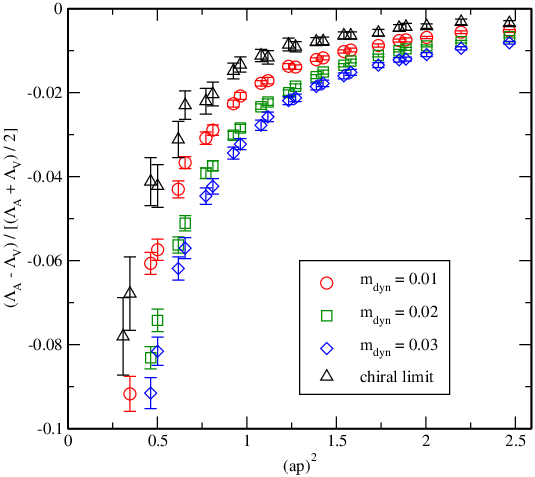
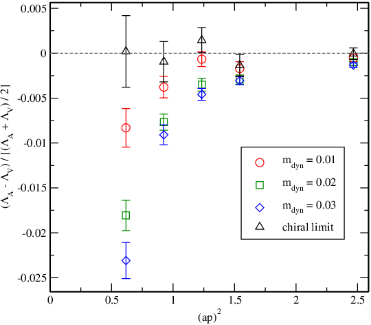
In practice, however, there are substantial physical spontaneous chiral symmetry breaking effects at low for standard RI-mom kinematics. These obscure a demonstration of the good chiral properties of DWF in coarse lattice spacing simulations. An example of this for the symmetry breaking splitting of in shown in figure 3. These effects also introduce an ambiguity in the determination of the renormalisation constants of around 2%. This physical effect is three orders of magnitude larger than any contamination expected from our residual chiral symmetry breaking , and no improvement will be gained by improving the accuracy of the chiral symmetry by either increasing or using a more exact overlap approach.
The problem has been enhanced by the particular choice of kinematics used in traditional RI-mom NPR. For a standard bilinear vertex function the leg momenta are equal and a soft subgraph is only suppressed by the of a single hard gluon as shown in figure 3.
A better alternative is to gain further suppression of soft contributions using non-exceptional momentum kinematics , figure 4.
Unfortunately the large body of higher perturbative calculations for various operators in RI-mom is non-trivial to reproduce for these alternative kinematics. However, use can be made of these results since even without conversion functions the good chiral chiral properties of DWF can be demonstrated and omission of chirality mixing for justified without requiring the perturbative conversion. There is no practical benefit, for these specific quantities, from further redution in . It is better to focus our available effort on more pressing problems. The great improvement in the scaling window we have demonstrated for RI-mom vertex functions with non-exceptional kinematics should serve as encouragement to the revisit high order calculations of the conversion to for non-exceptional kinematics. It is also quite possible that the convergence properties of the perturbative expansion will be improved in some cases. For example the four-loop Wilson coefficient relevant to displays much better convergence in than for conventional RI-mom.
Table 2 lists the axial current, field, mass, tensor and four quark operator renormalisation constants obtained in reference [38].
| 2 GeV | Z | stat | sys |
|---|---|---|---|
| 0.7161 | 0.0001 | ||
| 1.656 | 0.048 | 0.104 | |
| 0.7951 | 0.0034 | 0.0117 | |
| 0.9276 | 0.0052 | 0.0222 |

2.4 Topological tunneling
One of the principal attractions of dynamical fermion simulations with good chiral symmetry is the existence of a correct axial anomaly. However, this perfection of the action could easily be compromised by mundane algorithmic issues resulting in failure to sample the topological structure of the vacuum adequately. Problems arise with exact chiral symmetry since the sign function has a discontinuity which molecular dynamics updates will skip over for any non-zero timestep. Approximations to the sign function, DWF included, can involve a smooth transition over some eigevalue range, figure 5. Problems of this nature have not been observed with DWF simulations, and are unlikely to appear as the integration is problem free provided Healthy global topological charge histograms are obtained on our ensembles in figure 6 and the susceptibility is displayed in figure 7.

The molecular dynamics problems have resulted in two responses from the dynamical overlap community. The reflection-algorithm treats the lowest modes exactly using a particularly expensive approach, while others [29] have used an auxiliary pseudofermion determinant to freeze the global topological charge by suppressing the density of low modes of . Here, it is worth noting that the Zolotarev approximation to the sign function used has a coarse lower bound and does not differ greatly from the displayed in figure 5. In the language of the overlap, the key difference from the RBC-UKQCD approaches is that the authors of [29] suppress the density of low modes of in the region using an auxiliary fermion determinant, and it is then feasible to project and treat exactly the few remaining low eigenmodes of . This results in a fixed topology simulation with improved chiral symmetry. Similar approaches could equally well be combined with the DWF approximation [31, 32, 33, 34].
We estimate that DWF simulations are around five times cheaper than the five dimensional Zolotarev approach used in [29], and twenty times cheaper than the nested four dimensional approach.
As DWF shows, issues with integrability of the fermion contributions in molecular dynamics are likely either solvable or avoidable. We note that were the auxiliary determinant and projection dropped, then the remaining Zolotarev approximation would yield a very “domain-wall-like” simulation and tunneling would likely take place. Some thought has recently been given to developing algorithms that continue to tunnel topology in the presence of an auxiliary determinant [30].
A more fundamental problem is the increasing potential barrier introduced between topological sectors by the gauge action with increasing . Eq. 2.1 and discussion indicates that can be a qualitative guide to the near-zero mode density . Figure 7 shows that this, and we conjecture the tunneling rate per unit lattice volume, vanishes exponentially in the gauge coupling.
The trade off is clear: suppressing the low modes that mediate topology change and attempting to answer the difficult question about ergodicity of the simulation is one rational choice. RBC and UKQCD’s choice has been to accept a level of residual chiral symmetry breaking that is merely a minor irritant, but avoid questionable ergodicity and the risk of getting anomaly physics wrong in a particularly expensive fashion. This is also a substantially cheaper simulation, allowing more important systematic issues to be addressed.


3 Measurements
| mx,my | 0.001 | 0.005 | 0.01 | 0.02 | 0.03 | 0.04 |
|---|---|---|---|---|---|---|
| 0.001 | A,B ; 240 | 290 | 340 | 420 | 490 | 550 |
| 0.005 | A,B | A,B,C; 330 | 370 | 450 | 520 | 580 |
| 0.01 | A,B | A,B | A,B,C; 410 | 480 | 560 | 600 |
| 0.02 | A,B | A,B | A,B | A,B,C; 550 | 600 | 650 |
| 0.03 | A,B | A,B | A,B | A,B | A,B,C; 650 | 700 |
| 0.04 | A,B | A,B,C | A,B,C | A,B,C | A,B,C | A,B,C; 750 |
Table 3 gives a summary table of the mesonic measurements made on our ensembles. Further measurements have been made of nucleon two and three point functions, and static-light two and three point functions [9, 10]. Between 150 and 700 measurements have been made on each ensemble depending on the quantity, and valence pseudoscalar masses vary between 240 MeV and 750 MeV. Dynamical pion masses run from 330MeV to 650 MeV. Many more valence masses than dynamical masses are used to increase the amount of information in the chiral regime and are exploited in fits to partially quenched chiral perturbation theory [36], as highlighted by the masses quoted in red.
4 Chiral effective lagrangian
In this section we review the results presented in more detail by Meifeng Lin and Enno Scholz at this conference [2]. Two approaches to fitting our data for pion and kaon masses and decay constants to obtain the LEC’s of the chiral effective Lagrangian have been presented at this conference. The finite range of validity of chiral perturbation theory leaves such determinations from lattice (or indeed real world) data as something of an art. The rather massive real world kaon is neither unambiguously light nor heavy compared with chiral scales.
One approach is to fit the full SU(3)SU(3) chiral effective theory to data including the kaon as an active chiral pseudoscalar. A strength of lattice formulations, such as DWF, with controlled flavour symmetry is that the chiral perturbation theory can be decoupled from lattice artefacts in our simulated flavour content.
A good available alternative is to treat the kaon as a non-Goldstone boson, coupled to an effective SU(2)SU(2) theory. The analysis is applicable whenever , whether or not the kaon is heavy or light compared to other scales and we do not rely on chiral perturbation theory being convergent at kaon masses. The LEC’s will be strange mass dependent and, since the kaon is somewhat lighter than a typical chiral scale, the convergence of the chiral expansion controlled by these LEC’s may be correspondingly impacted. This will merely reflect the new dynamics that enters at the kaon mass scale. A reasonable estimate is that successive orders in the chiral expansion will only be suppressed by . To estimate possible systematic NNLO contamination entering when we perform SU(2) fits with a mass cut-off we multiply the size of NLO corrections in our NLO fit by . The relevant formulae can be easily obtained from standard SU(2) heavy meson chiral perturbation theory under the simplification that vector contributions are dropped[35].
We find that SU(3)SU(3) NLO partially quenched chiral perturbation theory [36] does not describe our data well up to meson masses comparable to the kaon mass. A good fit can only obtained with a cut in bare quark mass of . while the kaon corresponds to . The utility of SU(3)SU(3) ChPT at NLO is questionable; however we can quote LEC’s that fit the data for valence strange and light quark masses obeying the bound , and light dynamical quark masses but with a fixed dynamical strange quark mass of . These LEC’s may well differ from those that would be obtained in the unphysical true SU(3) chiral limit. The low energy constants obtained are displayed in table 4 for two popular choices of the chiral scale.
We also directly applied SU(2)SU(2) to fit the LEC’s of the effective two flavour theory that matches our simulated 2+1 flavour “real” world. These are also displayed in table 4. We fit the NLO forms to our data using a mass cut to obtain a good quality of fit. We perturbatively convert our results to the scale independent , SU(2) LEC’s in table 5. Interestingly our 2+1f results, both from a perturbatively converted SU(3) fit and from a direct SU(2) fit are broadly consistent with each other and with the 2f results of ETMC [40] and CERN [41, 42]. This adds somewhat to the picture discussed recently by Leutwyler [43].
| , conv. | 2.457(78) | 0.0661(18) | 2.87(28) | 4.10(05) |
|---|---|---|---|---|
| 2.414(61) | 0.0665(21) | 3.13(33) | 4.43(14) |
5 Quark masses and lattice spacing
We determine and from a combination of the S=3 baryon mass and the pseudoscalar kaon and pion masses. These quantities then produce the correct mass from linear extrapolation in the valence mass to and to in the light sea masses. They simultaneously produce consistent kaon and pion masses using our SU(2)SU(2) chiral extrapolations.
The scale from the can also be used to predict , , and the quark masses [2]. Based on our preliminary analysis our bare quark masses correspond to renormalised quark masses of and in the at 2 GeV. We find . We obtained MeV, , which are around 5% lower than their experimental values. This is likely an effect, and our ratio . This implies . Here the errors on decay constants are statistical only, and the quark masses and contain only partial systematic errors. Full systematic errors will be estimated in a journal paper [39].
The lattice spacing determined from is somewhat different, being around 1.65 GeV on and 1.62GeV on . While on we relied on vector meson states (which are unstable in QCD) and an ad hoc value of fm for to set the scale, our larger volume enables and baryon masses to be safely considered. We find broad consistency between decay constants and the Omega (which, being composed of three strange quarks, is physically small for a baryon). We have found that in the chiral limit , and this suggests we measure a physical value of fm, and disfavour fm. Were we to use the pseudoscalar decay constants to set the scale fm. This is a tendency that is consistent with other recent lattice calculations [37], and cautions against reliance on vector mesons for precision scale. We are encouraged by recent progress that has been made on treating vector meson decay in lattice QCD [44].
6 Neutral kaon mixing
We have updated our paper [12] on with results that have been presented by Cohen and Antonio at this conference [3]. We use the two wall, operator sink method to gain a spatial volume average. We use propagators that are the sum of solutions for periodic and anti-periodic temporal boundary conditions to eliminate unwanted round-the-world propagation. This gives exceedingly long plateaux on our lattice. We have modified our analysis to set the lattice spacing from the mass and now use fits assuming only SU(2)SU(2) chiral symmetry which we consider to be more theoretically robust. We have access to lighter masses and more statistically precise data and see evidence of curvature in the fixed strange mass chiral extrapolation. Partially quenched SU(2)SU(2) chiral perturbation theory both describes the valence and sea mass dependence well in the region of our fit. The smaller volume data point is not included in our fit, but the unitary fit curve matches onto this data point reassuringly well.

The final results follow, with the first error statistical and the second systematic.
| (3) | |||||
| (4) | |||||
| (5) |
The components of the systematic error are shown in table 7. These errors are added in quadrature, and the discretisation systematic is dominant. Simulations in progress with a finer lattice spacing will directly address this. The two-loop perturbative conversion to is currently a subleading error but will soon become the most important error to address. Finer lattice spacings will only yield logarithmic improvement, and a higher order calculation, preferably with non-exceptional momenta, is important. A non-perturbative step scaling approach could, of course, even better address the convergence of perturbation theory.
| Non-perturbative renormalisation | 2% |
| Sea strange mass adjust | 1% |
| Chiral extrapolation | 2% |
| Discretisation | 4% |
| Finite volume | 1% |
7 Kl3 form factor
James Zanotti presented a status update of our calculation of the semileptonic kaon decay form-factor[5], which is obtained from the matrix element of the weak vector current
This is a promising approach for an accurate determination of , and makes use of standard double ratio techniques [45] to measure the deviation of the form factor from unity, giving a very small overall error. An example ratio is given below.
Preliminary results using only the data points were presented in [17, 16]. We have now added the lightest data point () and finalised our analysis in a full paper [6]. The updated analysis includes unified chiral and extrapolations, using a fit form that combines a quark mass dependent pole dominance model with the constraints of the Ademollo-Gatto theorem:
| (6) |
The results from a fit to the large volume () data is presented in Fig. 9. The left and right plots show the and quark mass dependencies of Eq. (6), respectively. At the physical meson masses, we obtain
| (7) |
which very much favours Leutwyler-Roos [48] results over more recent higher order calculations [49, 50]. The first error in Eq. (7) is statistical, while the second is an estimate of the systematic error due to our choice of ansatz (6) and the third is the estimate of discretisation errors. The PDG quotes [46]22 2 A more recent analysis finds [47], so using our result (7), we obtain
Despite being less mature, Kl3 form factor appears very competitive with respect to as a lattice method for constraining .


We anticipate a substantial reduction in error by a recalculation with a combination of twisted boundary conditions [15] (removing the systematic uncertainty in the extrapolation) and stochastic volume averaging for our data point (reducing the error in the most important point in the chiral extrapolation). Finally, discretisation effects will be addressed before the next lattice conference using our new ensembles with a finer lattice spacing.
8 Pion and kaon distribution amplitudes
Chris Sachrajda presented [4] a calculation of the first and second moments of distribution amplitudes of the pion and kaon computed from the following matrix elements
This calculation was performed on our ensembles and follows on from an earlier work on [19, 18]. The first moment vanishes in the mass degenerate case and is non-zero for the kaon, figure 10, but not for the pion. The second moment has relatively weak mass dependence for both kaon and pion, figure 11. These were renormalised using one-loop lattice perturbation theory and we obtain the following preliminary results:


| (8) |
9 Vector meson decay constants
These are defined through
The vector meson decay consnant is well constrained experimentally, but the tensor current coupling is useful input that lattice gauge theory can provide to sum rules and other phenomenological applications. Chris Sachrajda presented a 2+1f DWF calculation of these transverse decay constants, renormalised with RI-mom NPR using both and volumes.
These results were obtained using only the input strange quark mass of , rather than the more physically realistic input quark mass (i.e. not including ) of . The ratios display very weak dependence on and an estimate absorbed this change in strange quark mass to the physical point. As the tensor current is scheme and scale dependent the final results were quoted at 2 GeV in the scheme as
| (9) |
In the scheme with GeV we finally obtain:
| (10) |
10 Nucleon mass and structure
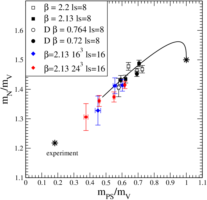
Takeshi Yamazaki and Shigemi Ohta have presented results [7] for isovector form factors and low moments of structure functions of the nucleon, and related work has also been discussed at other conferences [51, 52]. These are performed using our four ensembles and the corresponding Edinburgh plot [53] is displayed in figure 12.
Nucleon three point functions have been calculated using a source-sink time separation of 12. For our simulation we find, figure 13, that the axial charge appears flat except at our lightest datapoint, which is around 15% lower. Similar behavour was seen by RBC, at heavier masses on a 2-flavour DWF simulation. We believe this is a finite volume effect with the mass threshold determined by the volume. Our data point on our ensemble does not display this effect, but carries very large statistical errors. Figure 13 displays our results against , and is suggestive of mass dependent finite volume effects which appear to scale with and appear for . We observe similar behaviour if we plot the results with Wilson fermions by LHPC/SESAM and QCDSF in this fashion [7, 54, 55]. Improved statistics for the 2+1f measurements is important to clarify the one (statistically questionable) exception to this picture.
The lowest data point is omitted from an extrapolation, and obtained at the physical pion mass.


Results were also presented for the vector, axial, induced tensor and induced pseudoscalar form factors, some associated couplings (such as and the induced pseudoscalar coupling ) and corresponding mean squared radii. The momentum fraction, helicity fraction, transversity and twist-3 structure function moments were calculated.
11 Conclusions
RBC and UKQCD have exploited the PPARC, Riken, and SciDAC QCDOC machines in Edinburgh and Brookhaven to simulate dynamical domain wall fermions with realistic sea quark content. The analysis of the first lattice spacing GeV on a volume is well advanced with a broad and rich physics programme presented at this conference. The programme will continue to analyse two ensembles on a finer lattice spacing that are currently being generated. The physics parameters are very competitive despite the cost of the additional fifth dimension, with sea pion masses down to MeV and valence pions down to MeV. Partially quenched chiral perturbation theory is exploited in our analysis programme and enabled many more data points to be measured within the SU(2)SU(2) chiral regime. We have obtained results for the low energy constants of the chiral effective lagrangian, quark masses, , and from both and from Kl3. We find that very large lattice volumes may be required for non-spectral nucleon physics based on suspected finite volume effects in the nucleon axial charge.
12 Acknowledgements
I wish to thank my colleagues in the RBC and UKQCD collaborations whose work it has been my priviledge to review: Conrado Albertus, Chris Allton, Dave Antonio, Yasumichi Aoki, Christopher Aubin, Tom Blum, Ken Bowler, Michael Cheng, Norman Christ, Michael Clark, Saul Cohen, Paul Cooney, Chris Dawson, Luigi del Debbio, Michael Donellan, Mike Endres, Jonathan Flynn, Alistair Hart, Koichi Hashimoto, Tomomi Ishikawa, Taku Izubuchi, Xiao-Yong Jin, Chulwoo Jung, Andreas Jüttner, Tony Kennedy, Richard Kenway, Changhoan Kim, Min Li, Sam Li, Adam Lichtl, Hugo H M C Pedroso de Lima, Huey Wen Lin, Meifeng Lin, Oleg Loktik, Robert Mawhinney, Chris Maynard, Jun Ichi Noaki, Shigemi Ohta, Brian Pendleton, Chris Sachrajda, Shoichi Sasaki, Enno Scholz, Amarjit Soni, Aurora Trivini, Robert Tweedie, Jan Wennekers, Azusa Yamaguchi, Takeshi Yamazaki, and James Zanotti. We thank the QCDOC design team for developing with us the QCDOC machine and its software. This development and the computers used in this calculation were funded by the U.S. DOE grant DE-FG02-92ER40699, PPARC JIF grant PPA/J/S/1998/00756 and by RIKEN. This work was supported by DOE grant DE-FG02-92ER40699 and PPARC grants PPA/G/O/2002/00465 and PP/D000238/1. We thank the University of Edinburgh, PPARC, RIKEN, BNL and the U.S. DOE for providing the QCDOC facilities.
References
- [1] N. Christ and C. Jung, Computational Requirements of the Rational Hybrid Monte Carlo Algorithm, this conference PoS(LAT2007)028. RBC and UKQCD
- [2] M. Lin and E. Scholz, Chiral Limit and Light Quark Masses in 2+1 Flavor Domain Wall QCD, this conference PoS(LAT2007)120, arXiv:0710.0536 [hep-lat]. RBC and UKQCD
- [3] D. Antonio and S. Cohen, The Kaon Bag Parameter from 2+1 Flavor Domain-Wall Fermion Lattices this conference PoS(LAT2007), arXiv:0710.0422 [hep-lat]. RBC and UKQCD
- [4] C. Sachrajda et. al., Lattice Results for Vector Meson Couplings and Parton Distribution Amplitudes this conference PoS(LAT2007)369. RBC and UKQCD. arXiv:0710.0869 [hep-lat].
- [5] James Zanotti, this conference.
- [6] P. A. Boyle et al., arXiv:0710.5136 [hep-lat].
- [7] T. Yamazaki and S. Ohta Nucleon form factors and structure functions with dynamical domain wall fermions, RBC and UKQCD this conference PoS(LAT2007)165 & 157. [arXiv:0710.0422].
- [8] R. Mawhinney and S. Li, this conference.
- [9] C. Albertus, Y. Aoki, P. A. Boyle, N. H. Christ, L. Del Debbio, T. T. Dumitrescu, J. M. Flynn, T. Izubuchi, O. Loktik, C. T. Sachrajda, A. Soni and J. Wennekers, mixing with domain wall fermions in the static approximation, this conference, PoS(LATTICE 2007)376
- [10] Y. Aoki, this conference.
- [11] C. Allton et al. [RBC and UKQCD Collaborations], Phys. Rev. D 76 (2007) 014504
- [12] D. J. Antonio et al. [RBC and UKQCD Collaborations], arXiv:hep-ph/0702042.
- [13] D. J. Antonio et al. [RBC and UKQCD Collaborations], arXiv:0705.2340 [hep-lat].
- [14] D. J. Antonio et al. [RBC and UKQCD Collaborations], Phys. Rev. D 75 (2007) 114501
- [15] P. A. Boyle, J. M. Flynn, A. Juttner, C. T. Sachrajda and J. M. Zanotti, JHEP 0705 (2007) 016 [arXiv:hep-lat/0703005].
- [16] D. J. Antonio et al., PoS LAT2006 (2006) 101 [arXiv:hep-lat/0610080].
- [17] D. J. Antonio et al., arXiv:hep-lat/0702026.
- [18] P. A. Boyle, M. A. Donnellan, J. M. Flynn, A. Juttner, J. Noaki, C. T. Sachrajda and R. J. Tweedie, PoS LAT2006 (2006) 111 [arXiv:hep-lat/0610025].
- [19] P. A. Boyle, M. A. Donnellan, J. M. Flynn, A. Juttner, J. Noaki, C. T. Sachrajda and R. J. Tweedie [UKQCD Collaboration], Phys. Lett. B 641 (2006) 67 [arXiv:hep-lat/0607018].
- [20] M. A. Clark, A. D. Kennedy and Z. Sroczynski, Nucl. Phys. Proc. Suppl. 140, 835 (2005) [arXiv:hep-lat/0409133].
- [21] M. A. Clark and A. D. Kennedy, Phys. Rev. Lett. 98, 051601 (2007) [arXiv:hep-lat/0608015].
- [22] C. Urbach, K. Jansen, A. Shindler and U. Wenger, Comput. Phys. Commun. 174 (2006) 87
- [23] T. Takaishi and P. de Forcrand, Phys. Rev. E 73 (2006) 036706 [arXiv:hep-lat/0505020].
- [24] P. Hernandez, K. Jansen and M. Lüscher, Nucl. Phys. B 552 (1999) 363 [arXiv:hep-lat/9808010].
- [25] M. Golterman, Y. Shamir and B. Svetitsky, Phys. Rev. D 72 (2005) 034501 [arXiv:hep-lat/0503037], and references therein.
- [26] M. Golterman and Y. Shamir, Phys. Rev. D 68 (2003) 074501 [arXiv:hep-lat/0306002].
- [27] N. Christ [RBC and UKQCD Collaborations], PoS LAT2005 (2006) 345.
- [28] S. R. Sharpe, arXiv:0706.0218 [hep-lat].
- [29] H. Matsufuru, Exploring the chiral regime with dynamical overlap fermions this conference PoS(LAT2007).
- [30] M. Golterman and Y. Shamir, arXiv:0705.2928 [hep-lat].
- [31] P. M. Vranas, arXiv:hep-lat/0001006.
- [32] P. M. Vranas, Phys. Rev. D 74 (2006) 034512 [arXiv:hep-lat/0606014].
- [33] T. Izubuchi and C. Dawson [RBC Collaboration], Nucl. Phys. Proc. Suppl. 106 (2002) 748.
- [34] R. G. Edwards and U. M. Heller, Phys. Rev. D 63, 094505 (2001) [arXiv:hep-lat/0005002].
- [35] S. R. Sharpe and Y. Zhang, Phys. Rev. D 53 (1996) 5125 [arXiv:hep-lat/9510037].
- [36] S. R. Sharpe and N. Shoresh, Phys. Rev. D 64 (2001) 114510 [arXiv:hep-lat/0108003].
- [37] C. McNeile, arXiv:0710.0985 [hep-lat], PoS(LAT2007) this conference.
- [38] Y. Aoki, et. al. Non-perturbative renormalisation of the Quark Bilinear operators and using Domain Wall Fermions RBC and UKQCD collaborations, in preparation.
- [39] RBC and UKQCD collaboration, in preparation.
- [40] Ph. Boucaud et al. [ETM Collaboration], Phys. Lett. B 650 (2007) 304 [arXiv:hep-lat/0701012].
- [41] L. Del Debbio, L. Giusti, M. Lüscher, R. Petronzio and N. Tantalo, JHEP 0702 (2007) 056
- [42] L. Del Debbio, L. Giusti, M. Lüscher, R. Petronzio and N. Tantalo, JHEP 0702 (2007) 082
- [43] H. Leutwyler, arXiv:0706.3138 [hep-ph].
- [44] S. Aoki et al. [CP-PACS Collaboration], arXiv:0708.3705 [hep-lat].
- [45] D. Becirevic et al., Nucl. Phys. B 705 (2005) 339 [arXiv:hep-ph/0403217].
- [46] E. Blucher and W.J. Marciano, “, the Cabibbo angle and CKM unitarity”, PDG, 2006.
- [47] M. Moulson [FlaviaNet Working Group on Kaon Decays], arXiv:hep-ex/0703013.
- [48] H. Leutwyler and M. Roos, Z. Phys. C 25, 91 (1984).
- [49] J. Bijnens and P. Talavera, Nucl. Phys. B 669, 341 (2003) [arXiv:hep-ph/0303103].
- [50] V. Cirigliano et al., JHEP 0504, 006 (2005) [arXiv:hep-ph/0503108].
- [51] H. W. Lin, arXiv:0707.3844 [hep-lat].
- [52] H. W. Lin and S. Ohta, PoS LAT2006 (2006) 118 [arXiv:hep-lat/0610028].
- [53] RBC and UKQCD collaborations, in preparation.
- [54] D. Dolgov et al. [LHPC collaboration], Phys. Rev. D 66 (2002) 034506 [arXiv:hep-lat/0201021].
- [55] A. A. Khan et al., Phys. Rev. D 74 (2006) 094508 [arXiv:hep-lat/0603028].