Fluctuation-driven heterogeneous chemical processes
Abstract
We explore a new framework for describing the kinetics of a heterogeneous chemical reaction where two particles of the same chemical species form a reaction product of another chemical species on the surface of a seed particle. Traditional treatments neglect the effect of statistical fluctuations in populations. We employ techniques in a manner analogous to the treatment of quantum systems to develop a stochastic description of processes beyond the mean field approximation.
1 Introduction
Traditional models employing the evolution of the mean population of
species in a system provide a good enough description of various
physical processes such as heterogeneous chemical reactions and
heterogeneous nucleation of aerosols as long as the average particle
number is large. However, when the mean populations involved are
small we expect to see a significant deviation from the solution to
the classical equations.
As an example consider the chemical reaction of two hydrogen atoms
on the surface of a dust particle in interstellar space
[13]. Atoms can be adsorbed onto and evaporated from the
grain particle. The adsorbed molecules will diffuse on the surface
of the seed and eventually collide with another reactant to form
diatomic hydrogen. Under interstellar conditions the rate of the
adsorption of atoms will be small compared to the reaction rate. If
the mean population of hydrogen atoms is small, statistical
fluctuations brought about by gain and loss, and by the random
diffusion of atoms on the surface of the dust particle, are
important. Yet the traditional model does not include the treatment
of such fluctuations. Several attempts have been introduced to
resolve that problem; among them the Monte Carlo approach, the
modified rate approach, the direct master equation approach and the
Gauge Poisson representation approach
—see [9, 10] and [7]. Related studies
have been carried out in [4, 11].
Analytical solutions to a master equation approach have been found
for the steady state case[1, 8, 16]. Our
work is a first step to an alternative approach for describing the
kinetics of a heterogeneous chemical reaction which can be extended
to other areas where a similar problem occurs, for example when
computing the rate of nucleation processes taking place on small
particles. Again, the number of adsorbed molecules is small and
statistical fluctuations need to be taken into account. In
[16] the steady state solution was studied employing
a description using master equations instead of mean population
dynamics. A nucleation rate lower than the classical equations
predicted was obtained. Therefore, it is important to develop a
model by which we replace the classical equations with a set of
stochastic equations.
For the correct treatment of population fluctuations we employ
methods of Quantum Field Theory [5, 6]. Starting
from a master equation we introduce a spatial lattice where the
microstates of the system correspond to a set of occupation numbers
at each lattice site. A Fock space is constructed using annihilation
and creation operators at each lattice site. By means of this set-up
it is easy to show that the master equation is equivalent to a
Schrödinger equation with imaginary time. This enables us to
employ techniques originally developed in order to describe a
quantum mechanical system where the fluctuations are due to a
quantum uncertainty. We obtain the average particle population of
the classical many-body system by developing a mechanism for
computing expectation values of observables analogous to Feynman’s
path integral formulation [2, 18]. In this paper we
will not concern ourselves with renormalisation group analysis
although studies in that direction have been undertaken by various
people, for example [12, 15, 21]. Introducing
a stochastic variable [20], a mathematical trick —for
a nice review paper we refer to [23]— helps with
the evaluation of the expression for the expectation values. The
complex fluctuating solutions to a set of constraint equations,
which are stochastic partial differential equations, are then
averaged over all realisations of the stochastic noise. For
numerical investigations, the solutions to the constraint equations
can be generated by various numerical schemes [14]. The
path integral average is computed using Monte Carlo
methods[17]. The Code is written in C and computations do
not take longer than a few seconds up to a few minutes running on a
standard laptop.
In the sequel we will concentrate on a heterogeneous chemical
reaction where two reaction partners of the same sort of particle
type react on the surface of a seed particle to form a reaction
product.
For readers more interested in the physical content than in the
mathematical details of the formalism we recommend to skip the first
few pages and instead have a look at the most important equations on
page 8 and continue from there. Equation (42) which is a
path integral average (PIA) gives the average particle density of
the various chemical species once the complex, fluctuating solutions
to the constraint equations (40) and (41) have
been found and inserted into the PIA. Together with the correlations
(43) for the stochastic noise occuring in the PIA this forms
a complete set of equations.
2 Mathematical Techniques
2.1 Master Equation And Schrödinger-like Equation
We concentrate on chemical reactions of type , that is situations in which the atoms adsorb onto grain
particles where they can associate with themselves to produce
diatomic molecules. If the number of reactive species on an
individual grain is small, traditional rate equations will fail to
accurately describe the diffusive chemistry occuring on the surface
of the grain particle. We start our investigations by determining a
master equation that describes such a heterogeneous chemical
process.
A can be written as
| (1) |
where represents the
or from a microstate to a microstate and
is the probability to find the system in state . Considering a d-dimensional with lattice constant ,
the microstates correspond to the occupation numbers at each lattice site .
The chemical reaction of pairs of species to form a product of
species on a particle or droplet , , is
modelled by the following master equation
| (2) |
This equation describes the evolution of the probability
distribution for the total number of
adsorbed molecules of species and for the number of
reaction products of species . The symbols
denote the numbers of or molecules at lattice
site , respectively. The constants , and
are rate coefficients, is the diffusion
constant and stands for the volume of the droplet. The rate
coefficient is called , the rate
coefficient is called and
is known as the .
In our model, the chemical reaction is taking place on a
d-dimensional lattice,
allowing for multiple occupancy on each site. This configuration is also called .
The changes in population which we consider are caused by:
- (a)
absorption of a molecule of species A from outside the grain particle (first line in the above equation), and absorption of a molecule of species C from outside the grain (second line in the above equation),
- (b)
binary reaction on the surface of the grain (third and fourth line in the above equation),
- (c)
evaporation of a molecule of species A from the grain (fifth line in the above equation), and evaporation of a molecule of species C from the grain particle (sixth line in the above equation),
- (d)
particle hopping of a molecule of species A from site to site (seventh line in the above equation), and particle hopping of a molecule of species C from site to site (eighth line in the above equation),
- (e)
particle hopping of a molecule of species A from site to site (ninth line in the above equation), and particle hopping of a molecule of species C from site to site (last line in the above equation).
The summation in the
fourth and fifth line of the above equation (2) is taken
over nearest neighbour sites only. The factors
describe the number
of ways of choosing the particles involved in the considered
process. In the continuum limit the particle hopping from one site
to another corresponds
to the diffusion of the particles.
The initial condition is chosen corresponding to a Poissonian
distribution on each site
| (3) |
where is the average occupation number per
lattice site for the or particles respectively.
In the next step we will apply the methods of second quantisation
[5, 6]. We will rewrite the master equation as a
Schrödinger-like equation for a many-body wave function. This
approach can be justified by noting that, first of all, the master
equation is a differential equation of first order with respect to
time. The second reason to suggest the treatment of the master
equation according
to the second quantisation is that the master equation is linear in the probability.
In order to simplify the notation we will suppress the dependence on
space coordinates . We will be working
in an appropriate space, the . A Fock space
is a Hilbert space made from the
direct sum of tensor products of single-particle Hilbert spaces
| (4) |
with a symmetrising (for the case of bosons) or antisymmetrising (for the case of fermions) operator. The Fock space is constructed by introducing the following operators at each lattice site
which satisfy the commutation relationships
| (5) |
The is defined by
| (6) |
with
| (7) |
where denotes the vacuum state in a
single-particle Hilbert space.
The master equation (2) is equivalent to the
Schrödinger-like equation —a Schrödinger equation with
imaginary time—
| (8) |
with the many-body wave function
| (9) |
and the Hamiltonian operator
| (10) |
For verification of the above statement one has to insert the states on both sides of the master equation — equation (2)— and sum over the set of all occupation numbers and . In general, the time-evolution operator is not necessarily Hermitian. For the timebeing let us suppress the subindices that identify the particle type. The form of the many-body wave function (9) can be made plausible when considering the state vector at site , namely
| (11) |
It holds that
| (12) |
2.2 Expectation Values Of Observables
We are interested in obtaining the expectation values for various observables, especially the average number density. The expectation values of observables are given by
| (13) |
We want the expectation values of the observables —diagonal in the occupation number basis— to be linear in the probabilities. After some straightforward computation —see for example [23]— one can see that the above expression is equivalent to
| (14) |
where
| (15) |
The projection state obeys the relation
| (16) |
By definition, the projection state is a left eigenstate of all creation operators with unit eigenvalue
| (17) |
Furthermore, . Conservation of probability requires that .
We break the time interval into T short slices of
duration . At each time slice we insert
a complete set of coherent states —see, for example,
[2]. Coherent states, , are
right eigenstates of the annihilation operator
| (18) |
where the eigenvalue is a complex function. The duals are left eigenstates of the creation operator
| (19) |
We have
| (20) |
The coherent states are over-complete. Still, we can use them to create the identity
| (21) |
for a single lattice site , and for multiple lattice sites accordingly
| (22) |
with . Let us recall the formula for the expectation values of observables
| (23) |
where the initial many-body wave function takes the form —see equations (3) and (9)—
| (24) |
We observe the following proportionalities
| (25) |
for all admissible values of . Therefore, one can recast the equation for the expectation values (23) into
| (26) |
where
| (27) |
for all admissible values of . According to the breakage of the time interval into time slices of small duration we rewrite the expression
| (28) |
occuring in the equation for the expectation values (26) and insert the identity as defined in (22) between each factor. Then the discrete version of the expectation values of operators reads
| (29) |
where we have labeled each time slice by a time index . The normalisation constant has to be determined lateron. The consideration of the lattice expectation value is not sufficient if one is interested in long wavelength properties. In the formal continuum limit, we obtain
| (30) |
Next, we expand the exponential function for small
, neglect higher order terms in and recast the
continuous average. When interested in inclusive probabilities
—e.g. the average number of particles at a given lattice site
irrespective of the number of particles elsewhere— it is
convenient to commute the factor of through the
operators and in . This has the effect of shifting using .
The operators are now normal ordered. It is valid that the operator
and its normal ordered counterpart have the same
expectation value if all creation operators occuring in the normal ordered operator are replaced by unity
—see for example [23]. In particular, the density
operator reduces to the annihilation operator . Therefore, in the continuum limit
the average particle density of the
particles is given by the stochastic average of the complex
eigenvalues of the coherent state vectors under the annihilation
operator, that is one chooses the operator to be
.
We take the continuum limit —the dimensions of the constants are
chosen by looking at the discrete Hamiltonian operator
(10)— via ,
,
, , ,
, and finally , where the newly introduced constants have the
following dimension properties ,
, ,
and in
Standard International units. The objects
and are
dimensionless. Notice that now scales
like a density.
In the continuum limit, the average particle density in the
stochastic model is then given by
| (31) |
where denotes the of the functional integral and is the of the dual of the coherent state under the creation operator defined by . Accordingly, all fields that incorporate shifted eigenvalues instead of the original eigenvalues will be denoted by a twiddle in the sequel. Note that the average (31) is performed taking into account the dynamics and the initial conditions —for a more detailed discussion see [23]. We already have incorporated the shifted initial state
| (32) |
in the shifted action . The symbol represents the which is defined as follows
| (33) |
with the shifted Hamiltonian . The shifted action for the chemical reaction takes the form
| (34) |
We want to untangle the quadratic term . A linear expression in can be obtained by means of a Gaussian transformation
| (35) |
where is the probability distribution for a white noise . The Gaussian distribution reads
| (36) |
Now the shifted action is linear in and one can easily integrate out over and in (31). One obtains
| (37) |
where is a functional Dirac delta distribution. In its generalised Fourier representation it is defined by
| (38) |
with being a multicomponent field satisfying the constraint
| (39) |
Accordingly, the functions and satisfy the constraints
| (40) | |||
| (41) |
It follows from equation (37) that the average particle density for the A respectively C molecules is now given by
| (42) |
The stochastic noise has zero mean value and a correlation given by
| (43) |
This is obvious when considering the Gaussian distribution
(36). Note that the above average is no longer taken over
the initial conditions.
The constraint equation (40) is an inhomogeneous partial
stochastic differential equation with additive noise for a complex
fluctuating unknown field in the It calculus. It
resembles the deterministic partial differential equation that
describes the evolution of the mean particle density in the
classical theory. But despite the temptation for an intuitive
interpretation it is very important to keep in mind that in equation
(40) we are confronted with a complex fluctuating quantity
that has as such no physical interpretation. Only if the path
integral average (PIA) (42) of a solution to
(40) or (41) is taken over all possible
realisations of the stochastic noise that appears in the constraint
equation can one interpret the outcome of this computation as a mean
particle density.
3 Case A: Vanishing Source Rate
In the remainder of this paper, let us concentrate on a single spatial site model. We will now compare the results in the stochastic model to the observations made in the traditional approach. The classical equation for the evolution of the mean particle density in the single spatial site model reads
| (44) |
where denotes the mean particle density of the molecules in the mean field approximation. The classical evolution equation (44) is solved by
| (45) |
The stochastic constraint equation for the complex fluctuating field in zero spatial dimensions with vanishing source rate takes the form
| (46) |
The traditional equation for the average particle density of the A molecules in the mean field approach (44) and the stochastic constraint equation associated with the A molecules (46) resemble each other at first sight. But as mentioned before the solution of the stochastic differential equation (46) is a complex, fluctuating field that can only be interpreted as an average particle density after it has been averaged in the sense of equation (42). For vanishing source rate it is fairly easy to find an analytic solution of equation (46). The stochastic constraint equation (46) —because of the continuous but not smooth nature of a stochastic process— has to be understood in terms of a stochastic integral equation
| (47) |
where
| (48) |
The stochastic noise is rewritten in terms of the Wiener process
| (49) |
For vanishing source rate the stochastic constraint equation for the particle density (40) reduces to the following equation
| (50) |
The above equation is a nonlinear reducible stochastic differential equation with polynomial drift of degree two in the It picture. In contrary to a Stratonovich stochastic differential equation an It stochastic differential equation can not be solved directly by methods of classical calculus11 1 Sample paths of a Wiener process are —with reasonable certainty— neither differentiable nor of bounded variation. As a consequence one is left with different interpretations of stochastic equations, namely the It and the Stratonovich interpretation. For a further reading we refer to [14].. For an analytical solution of an It stochastic differential equation one has to use a modified version of the drift coefficient
| (51) |
where the derivative in the last term is a functional derivative. Equation (50) is a stochastic version of a Verhulst-like equation —see [14]. It can be reduced to a linear stochastic differential equation with multiplicative noise. We obtain the solution to the first stochastic constraint equation (40) for vanishing source rate, namely
| (52) |
Inserting the above solution into the path integral
average (42) one obtains the average particle density for
the molecules in the stochastic picture.
The stochastic constraint equation for the reaction product, the
particles, in zero dimensions looks —in its form— identical to
the classical evolution equation for the mean density of
particles
| (53) |
In the single spatial site model, the full solution of the second constraint equation —simply take instead of in the above equation (53)— can be obtained even for non-vanishing source rate and reads
| (54) |
The stochasticity of the above equation is hidden in the
first term employing the fluctuating solution of
the first constraint equation (46).
Once the solutions to the stochastic constraint equations
(52) and (54) are known, one has to insert either
of the solutions into the path integral average (42) and
compute the path integral by means of a Monte Carlo calculation in
order to obtain the average particle density for the or
particle population, respectively. Random samples are generated
according to the Gaussian probability distribution (36);
that is we generate Wiener processes. We estimate the path integral
(42) by summing a large number of solutions of the
constraint equations associated to the set of random samples
generated in the above sense and divide the sum by the number of
random samples. The Monte Carlo method displays a convergence of
where is the number of random samples
—see [19].
Instead of using the expressions of the
analytical solutions, equation (52) and equation
(54), to generate solutions to the stochastic constraint
equations one can alternatively compute the paths directly from the
stochastic differential equations (40) and (41).
The latter method turns out to be less time consuming. The
stochastic differential equation (40) in zero dimensions
can be converted into
| (55) |
where in discretised time for , and . The is generated by two uniformly distributed independently random variables via the Box-Muller transformation —see, for example, [14]. The numerical scheme (55) is called the Euler scheme and is the most straightforward approach to undertake some numerical investigations. Accordingly, the second constraint equation in the single spatial site model and for vanishing source rate takes the following form
| (56) |
As stochastic differential equations are extremely
sensitive one has to convince oneself that the code is stable and
converging as it should be. Other schemes we used that might be more
accurate or stable than the Euler method are the Milstein scheme,
the simplified order 2.0 weak Taylor scheme, the implicit order 1.0
strong Runge-Kutta scheme, the predictor-corrector method of order 1
with modified trapezoidal method weak order 1.0 —see
[14].
For the numerical evaluation we employ values for the rate
coefficients that can be found in realistic physical set-ups.
Instead of using the coefficients introduced in the continuum limit,
namely and , we employ the
traditional rate coefficients which we denote by and
and which have dimensions per unit time. Dimensional
analysis shows that using these new constants we are now calculating
an average particle population instead of an average particle
density —this can be easily verified in equations (46)
and (53).
The following plots were generated for the situation where two
hydrogen atoms react on the surface of an interstellar dust
particle. According to [3, 22] the
reaction rate takes the value of ,
the evaporation rate for the hydrogen atoms and the evaporation rate for the reaction product
. As initial values we used
.
In Figure 1 we generate the real part of one solution to the
stochastic constraint equation for the hydrogen atoms under the
above conditions. Figure 2 shows the imaginary part of the same
solution of the stochastic constraint equation for the reaction
partners. If one compares these plots to Figure 3 and Figure 4 where
the real and imaginary part of the path integral average over 1000
realisations of the white Gaussian noise for the atoms are given
one observes that the real part of the path integral average
smoothes out and the fluctuations in the imaginary part decrease in
intensity. For increasing number of paths employed in the path
integral average the imaginary part of the PIA tends to zero.
Therefore, it is safe to interpret the real part of the path
integral average as the average particle population.
Figures 5 and 6 show the real and imaginary part of a solution to
the second stochastic equation that constrains the reaction products
. Again the fluctuations are smoothed out in Figure 7 and
Figure 8 when the path integral average for the diatomic hydrogen is
taken over 1000 realisations of the stochastic noise.
Together with Figure 7 one can interpret the path integral average
in Figure 3 in the following way: according to Figure 7 the chemical
reaction stops after certain transient processes. The average
population of the diatomic hydrogen is constant. The intuitive
physical reason for this is because all the potential reaction
partners have already been used to form the reaction product
. On the other hand, from Figure 3 one sees how the plot for
the hydrogen atoms approaches asymptotically the value one half
which could be interpreted as a state consisting of either zero or
one particle. The value of is the
lowest possible eigenvalue of the coherent states under the
annihilation operator once the system has reaches its equilibrium.
The rate coefficients and have to be understood in a
probabilistic sense, in a similar fashion as it is done with, say,
the mean life expectancy of a radioactive isotope.
For the specific values we used in our calculations the reaction
rate dominates over the evaporation rate.
The discussion above
can be compared with the results obtained from the solution to the
classical evolution equation (45) which predicts an
asymptotic value as for . That is, the classical model predicts the
extinction of all the reactants.


4 Case B: non-vanishing source rate
As in the previous section, we generate solutions to the constraint equations (40) and (41) in zero dimensions by the numerical schemes discussed above but now with a non-zero source rate. We compare the results to the solutions of the classical evolution equations which read
| (57) |
where and and
| (58) |
We now analyse the influence of the source rate
coefficient associated with the adsorption of reactants onto the
surface of the seed particle. For convenience, we will leave the
source rate for the reaction products at zero as it will not have
significant influence on the outcome of our discussion. The other
rate coefficients were chosen as before, , and
denoting the rate coefficients per unit time. The plots in
Figures 9 to 12 were obtained for a source rate that is big in
comparison to the other rate coefficients, ,
whereas in Figures 13 to 16 the source rate was chosen to be small,
. Although one observes fluctuations both in
the real part of a single solution to the first constraint equation
(Figure 9) and in the real part of one path associated with the
second constraint equation (Figure 11), Figures 9 to 12 reproduce
deterministic behaviour. The real part of the path integral average
of the reactants (Figure 10), as well as the real part of the path
integral average of the reaction products (Figure 12) over 1000
possible realisations of the stochastic noise, coincide with the
results of the associated classical equations. This accordance
between classical and stochastic model is no longer valid for
Figures 13 to 16. As an example, we generated one single path for
each particle population, the reaction partners and the reaction
products, and plotted their real part in Figure 13 and Figure 15,
respectively.
Let us now compare the average particle
populations of the hydrogen atoms and the diatomic hydrogen for
large source rate (Figure 10 and Figure 12) to the average particle
populations of the reactants and the reaction product for small
source rate (Figure 14 and Figure 16). In the deterministic case,
that is for large source rate, the chemical reaction does not die
out after a certain period of time
—see Figure 12— in contrary to the observations made from Figure
16 where the real part of the path integral average of the diatomic
hydrogen over 1000 paths is plotted for a small source rate. As can
be seen from Figure 10 and Figure 14 respectively, for a source rate
of the average particle population of the
atoms reaches an asymptotic value of whereas for a source
rate of the average particle population of
the atoms is as was the case for vanishing source rate in
the latter section. Figure 12 and Figure 16 give the average
particle population for the atoms at time
, namely for large source rate
and for small source rate . To
determine the transition from a deterministic to a stochastic
behaviour we computed the average particle population of the
reaction partners and products for a source rate of the hydrogen
atoms in the range of
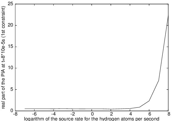
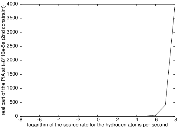
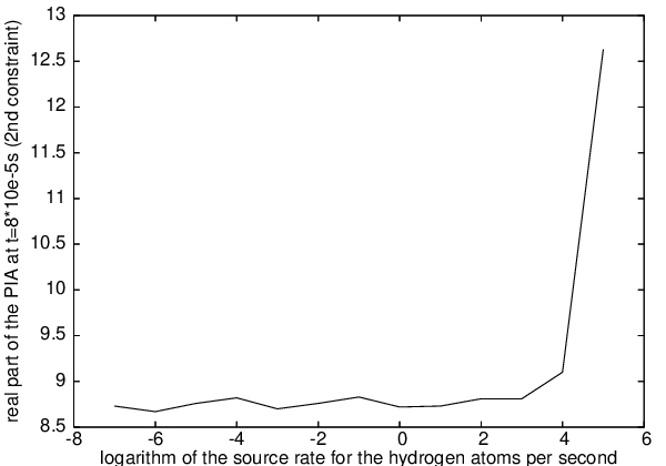
for each order of magnitude and generated Figure 17 to Figure 19.
Already when the reaction rate and the source rate are of the same
order of magnitude one can observe deviations from the classical
behaviour, in the sense that the equilibrium value of the average
particle population obtained by the stochastic methods is higher
than that predicted from the classical equation (57). One
also observes from Figure 17 that for a source rate between
and the chemical reaction
dies out because there is not one pair of reaction partners left in
order to initiate a chemical reaction.


5 Conclusions
We have argued that the classical evolution equations for the mean
particle population of a chemical species involved in a
heterogeneous chemical reaction do not give the right results for
small systems. Instead, we developed a stochastic model that
includes statistical fluctuations and showed in our numerical
investigations that those fluctuations can not be ignored for low
rates of particle adsorption onto the surface of a grain particle.
Although one starts from an apparently classical system the
introduction of a quantum field theoretical formalism for its
description seems to force us to adopt a ”quantum mechanical-like”
interpretation of the results.
It is possible to extend this work to other chemical reactions, for
example of the type . In a next step, we
shall consider a network of chemical reactions in which several
reactions compete against each other. One would expect that it will
take considerably longer to reach an asymptotic value for the
average particle population of a certain species.
6 Acknowledgements
This work was supported by the Leverhulme Trust under grant F/07134/BV and partly supported by the C N Davies Award of the Aerosol Society.
References
- [1] O. Biham & I. Furman, Master equation for hydrogen recombination on grain surfaces, The Astrophysical Journal 553, 595–603 (2001).
- [2] J. P. Blaizot & H. Orland, Coherent states: Applications in Physics and Mathematical Physics, page 474, World Scientific, 1985.
- [3] P. Caselli, T. I. Hasegawa, & E. Herbst, A proposed modification of the rate equations for reactions on grain surfaces, The Astrophysical Journal 495, 309–316 (1998).
- [4] O. Deloubrière, L. Frachebourg, H. Hilhorst, & K. Kithara, Imaginary noise and parity conservation in the reaction , Physica A 308, 135–147 (2002).
- [5] M. Doi, Second quantization representation for classical many-particle systems, Journal of Physics A: Math. Gen. 9(9), 1465–1477 (1976).
- [6] M. Doi, Stochastic theory of diffusion-controlled reaction, Journal of Physics A: Math. Gen. 9(9), 1479–1495 (1976).
- [7] P. Drummond, Gauge Poisson representations for birth/death master equations, Eur. Phys. J. B 38, 617–634 (2004).
- [8] N. J. B. Green et al., A stochastic approach to grain surface chemical kinetics, A & A 375, 1111–1119 (2001).
- [9] E. Herbst, The chemistry of interstellar space, Chem. Soc. Rev. 30, 168–176 (2001).
- [10] E. Herbst & V. I. Shematovich, New approaches to the modelling of surface chemistry on interstellar grains, Astrophysics and Space Science 285, 725–735 (2003).
- [11] D. Hochberg, M.-P. Zorzano, & F. Morán, Complex noise in diffusion-limited reactions of replicating and competing species, Phys. Rev. E 73, 066109 (2006).
- [12] M. Howard & J. Cardy, Fluctuation effects and mulitscaling of the reaction-diffusion fron for , J.Phys.A:Math.Gen. 28, 3599–3621 (1995).
- [13] W. Klemperer, Interstellar Chemistry Special Feature: Interstellar Chemistry, PNAS 103, 12232–12234 (2006).
- [14] P. E. Kloeden & E. Platen, Numerical Solution of Stochastic Differential Equations, Springer, 1992.
- [15] B. P. Lee, Renormalization group calculation for the reaction , J.Phys.A:Math.Gen. 27, 2633–2652 (1994).
- [16] A. A. Lushnikov, J. S. Bhatt, & I. J. Ford, Stochastic approach to chemical kinetics in ultrafine aerosols, Journal of Aerosol Science 34, 1117–1133 (2003).
- [17] N. Metropolis et al., Equation of state calculations by fast computing machines, J. Chem. Phys. 21(6), 1087–1092 (1953).
- [18] L. Peliti, Path integral approach to birth-death processes on a lattice, J.Physique 46, 1469–1483 (1985).
- [19] W. H. Press et al., Numerical Recipes in C, Cambridge University Press, second edition, 1992.
- [20] P.-A. Rey & J. Cardy, Asymptotic form of the approach to equilibrium in reversible recombination reactions, Journal of Physics A: Math. Gen. 32, 1585–1603 (1999).
- [21] P.-A. Rey & M. Droz, A renormalization group study of a class of reaction-diffusion models, with particles input, J.Phys.A: Math. Gen. 30, 1101–1114 (1997).
- [22] T. Stantcheva, P. Caselli, & E. Herbst, Modified rate equations revisited. A corrected treatment for diffusive reactions on grain surfaces, A & A 375, 673–679 (2001).
- [23] U. C. Taeuber, M. J. Howard, & B. Vollmayr-Lee, Applications of field-theoretic renormalization group methods to reaction-diffusion problems, J Phys. A: Math. Gen. 38, R79–R131.