A Weyl function approach to matter-wave coherence and Talbot-Lau effects
Abstract
Weyl functions conveniently describe the evolution of wave coherences in periodic or quadratic potentials. In this work we use Weyl functions to study the “Talbot-Lau effect” in a time-domain matter-wave interferometer. A “displacement diagram” is introduced to analyze and calculate the matter-wave interference for an atomic cloud in a quadratic potential that interacts with a sequence of short optical standing wave pulses producing an atomic grating echo. Unlike previous treatments, this new approach allows the atomic ensemble to have an arbitrary initial phase-space distribution, and the standing wave grating vectors to span three dimensions. Several examples are discussed to illustrate the convenience of the diagrammatic technique including the following: a two-dimensional Talbot-Lau effect, the shift in the echo time and the recoil phase for the interferometer perturbed by a quadratic potential; and the realization of a time-domain “Lau effect” using a pulsed harmonic potential. The diagrammatic technique is applicable to diffraction gratings with arbitrary grating transmission functions. We conclude the paper with a general discussion on the Weyl function representations of matter-wave coherence, and relate the conservation of matter-wave coherence with the conservation of purity that distinguishes decoherence effects from dephasing effects.
pacs
39.20+q, 03.75.dgI Introduction
In quantum phase space methods, operators in a Hilbert space are mapped to functions in a “mock” phase space Balazs and Jennings 1984. One example is the Wigner representation which is particularly useful for establishing quantum-classical correspondence. In the Wigner representation, the Wigner function represents a density matrix operator with a quasi-probability distribution in classical phase space. The Wigner functions are conveniently applied in semiclassical methods Heller 1976; Berry 1977, to visualize or characterize quantum states, and experimentally allows one to recover information of quantum systems through tomographic measurements of their phase-space distributions Smithey et al. 1993.
In the related Weyl function representation Balazs and Jennings 1984; Bishop and Vourdas 1994, the Hilbert space operators are mapped to functions in a “reciprocal phase space” where each function is simply a Fourier transform of those in the Wigner representation. In particular, Weyl function is the Fourier transform of the Wigner function over the phase space coordinates Vourdas 2006; Chountasis and Vourdas 1998. The Weyl function can also be expressed as:
| (1) |
Here and are the position and momentum operators, and is the displacement operator Bishop and Vourdas 1994, that shifts the density matrix by in momentum and in position. Thus the Weyl function is a phase-space correlation function that measures the coherence of matter-waves. Though both Weyl and Wigner functions completely specify any density matrix operators, application of Weyl function, or the Fourier transform of the Wigner function, has been much less discussed before Chountasis and Vourdas 1998.
In this work, we demonstrate the power of the Weyl function technique by applying it to an important class of wave interference phenomena, the Talbot-Lau effects associated with matter-waves in quadratic or periodic potentials. Various examples of Talbot-Lau type interference, including those closely related to recent experiments Su et al.; Wu et al. 2007; Wu 2007, are discussed. To our knowledge, this work gives the first vectorial and diagrammatic formula of Talbot-Lau effects. Apart from the expected application in matter-wave optics, the formula may also provide a convenient framework for the design of various lens-less imagine systems Pfeiffer et al. 2006.
I.1 Talbot-Lau effects
Periodic light wavefronts can repeatedly reconstruct themselves during free propagation. The phenomena is known as the Talbot effect that was discovered by Henry F. Talbot Talbot 1836 in 1836. A demonstration of the Talbot effect usually starts with a collimated monochromatic light with wavelength . The light passes through a transmission grating with a grating constant to generate a periodic wavefront. Full or partial re-constructions of the transmission wavefront at integer or fractional multiples of the Talbot distance are observed downstream. Many intricate and elegant features of the Talbot phenomena have been discussed in the literature Berry 1996. Instead of using a collimated or spatially coherent input, in 1948 Ernst Lau Lau 1948 found that spatially incoherent light, propagating through two gratings with same grating constant separated by a distance , can generate an interference pattern at the focal plane of a lens (Fraunhofer diffraction) placed downstream from the second grating. The contrast of the interference is maximized if takes integer multiples of . More general than Fraunhofer diffraction, in the Lau effect the interference pattern appears at a distance downstream from the second grating where are two integers. Lau’s original discovery corresponds to Lau 1948; Jahns and Lohmann 1979.
Instead of using light waves, both the Talbot Chapman et al. 1995; Deng et al. 1999 and the Lau effects Clauser and Li 1994 have been demonstrated using matter-waves and in particular using neutral atoms. Interferometry with multiple gratings using the Lau effect is referred to as Talbot-Lau or Talbot-vonLau Interferometry (TLI). The Lau effect is of particular interest for observing matter-wave interference in the circumstances where a bright and collimated matter-wave input is not available. Talbot-Lau interferometers are used to demonstrate wave properties of atoms and molecules AIBerman; Chapman et al. 1995; Clauser and Li 1994; Brezger et al. 2002a; Hackermuller et al. 2003a, to study decoherence Hackermuller et al. 2003b; Hornberger et al. 2005 and to measure the polarizability of large molecules Berninger et al. 2007. Talbot-Lau interferometers have also been explored to sense inertial forces with matter-waves Fray et al. 2004; Cahn et al. 1997; Weel et al. 2006; Wu et al. 2007; Wu 2007.
Based on Fresnel diffraction, matter-wave Talbot and Lau effects can also happen in the time domain instead of in the spatial domain, due to the equivalence of Schödinger’s equation and the paraxial wave equations. Matter-wave Talbot Deng et al. 1999 and Lau Cahn et al. 1997 effects in the time domain have been observed with atoms cooled down to a thermal velocity of centimeters per second or lower. In the time domain, spatially separated gratings are replaced by successive pulses of optical standing waves acting as either phase or amplitude gratings for the matter-waves. Time-domain interferometry using optical standing wave pulses with laser-cooled atoms were pioneered by the authors of ref. Cahn et al. 1997. In that experiment, off-resonant standing wave pulses act as thin phase gratings to an atomic cloud. After each standing wave pulse the atoms bunch to the potential minima of the standing wave to form a density grating. The density grating washes out due to velocity spreading of atoms. However, with two successive standing wave pulses separated by time applied to atoms, the atomic density grating revives around time if and more generally if , where is an integer. The contrast of the revived density grating is a periodic function of , similar to the spatial Lau effect. The revived atomic density grating is probed using a Bragg-scattering of a probe light to induce a grating echo Mossberg et al. 1979, and the interferometry based on this setup is referred as a time-domain grating echo interferometer Weel et al. 2006. Experiments and the theory of the interferometry were further developed in ref. Strekalov et al. 2002 that generalizes the technique to include multiple standing wave pulses. Recently a direct spatial image of sub-wavelength spatial interference pattern due to the Lau effect after two standing wave pulses (act as either amplitude or phase gratings) is achieved using an on-resonant standing wave mask Turlapov et al. 2005; Tonyushkin and Sleator 2006.
Developed theories of matter-wave Talbot-Lau effect (TLE) usually simplify the analysis by making particular assumptions on the coherence properties of input matter-waves. Closely related to the spatial (beam) Talbot-Lau setup with amplitude transmission gratings, in the first approach Carnal et al. 1995; Brezger et al. 2002b; Clauser and Reinsch 1992 the atom flux through each opening of the first grating are treated essentially as individual point sources, from which the Fresnel diffraction on the image plane is calculated. An incoherent sum of the contribution from all the openings at the grating gives the final interference pattern. Instead of incoherent summation of point sources, the second approach AIBerman; Strekalov et al. 2002; Dubetsky and Berman 1999 assumes the input atoms as an incoherent sum of plane waves. However, a general theory of Talbot-Lau interferometry applicable to matter-waves with arbitrary initial spatial coherence hasn’t been presented in the literature.
The approach to TLE in this work is motivated by an obvious link between the Weyl function [Eq. (1)] and the time-domain matter-wave TLE due to a sequence of standing wave pulses. In the following we consider a single atom picture with atomic motion characterized by a density matrix operator . TLE corresponds to a revival of atomic density grating at a certain time t. Since the revived density grating is spatially periodic, we shall consider its particular component given by:
| (2) |
where is the Weyl function defined in Eq. (1).
To express Eq. (2) in terms of an arbitrary initial condition described by , one can propagate forward in time by considering the interaction of atoms with a sequence of standing wave pulses. Alternatively, we shall define the time-dependent displacement operator in the Heisenberg picture and propagate the displacement operator backward in time. Here we take the latter approach which is advantageous for two reasons: 1) It applies to general initial conditions. 2) As we will see, the equation of motion for due to pulsed periodic potentials, during free-propagations and due to a quadratic potential can be integrated easily. Since our analysis is generally applied to different types of interferometers using TLE, we shall generally consider an interferometry configuration using TLE as a Talbot-Lau Interferometer, that will be referred to with the abbreviation TLI in this work.
I.2 Outline
In what follows the paper is organized into three sections. In the first section we introduce a diagrammatic technique to calculate the grating echo of an N-pulse TLI in free-space. In the second part we discuss the application of the theory to matter-waves in a quadratic potential. In the discussion section we extend the formula to include arbitrary grating transmission functions, discuss the Weyl function representation of matter-wave coherence, and compare the approach here with other diagrammatic techniques Beach et al. 1982.
II Grating echo due to TLE in free space
II.1 The model

In this section we consider TLE due to the simplest possible interaction between 2-level atoms and a sequence of off-resonant standing wave light pulses. The scenario is summarized in Fig. 1: an atomic sample localized at the waists of multiple standing wave fields is subjected to a sequence of N-1 standing wave pulses. At time a grating echo is induced with the amplitude proportional to a particular spatial Fourier component of the revived atomic density grating. The assumptions in the model are summarized below. For notational convenience, we set .
- A1.
2-level atoms are always in their adiabatic ground state, with any spontaneous light scattering ignored. Standing waves pulse with the time-dependent light shift Happer and Mathur 1967 potential acts as a phase grating to atoms. Here is the k-vector of the standing wave. , are the k-vectors of the traveling wave light fields, whose electric field amplitudes are referred to as and . And determines the position of the standing wave nodes in the lab frame. We assume the light fields have Gaussian beam profiles and the atomic sample is located at the center of each beam. The cross-sections of all the beams are characterized by a waist size , that is much larger than the size of the atomic sample. We also assume all the and to have significant differences in propagation directions such that any linear combinations of s have magnitude either zero or on the order of , with the optical wavelength.
- A2.
Standing wave pulses are in the Raman-Nath regime, e.g., the positions of atoms are considered frozen during each pulse duration. We thus can use Dirac delta functions to effectively describe the temporal profile of the pulses, e.g., that is characterized by its strength and the time of arrival . is referred as the pulse area.
- A3.
The atomic ensemble is assumed to be dilute such that atom-atom interactions are ignored. The ensemble is assumed to be dilute in phase space as well so that the single atom picture is applied without conflicting with quantum statistics. We can thus use a Dirac ket to label the matter-wave state, that obeys the single atom Schrödinger’s equation,
(3) Given a fixed amount of atoms participating in the interaction, the spatial density distribution of the atomic ensemble is given by , where is the single atom density matrix for the atomic ensemble in real space. Impacts of on the matter-wave dynamics require only relatively simple algebra, so we may drop during the derivation and recover their values if necessary.
- A4.
A grating echo refers to the Bragg scattering of probe light pulse (the last graph in Fig. 1) off the revived atomic density grating. The amplitude of the grating echo is evaluated under first order Born approximation. We assume the evolution of the atomic density grating is not perturbed by the scattered light during the probing interval. Using a slowly varying amplitude approximation, the coupling between and the probe light field around time is governed by the equation:
(4) Here measures the distance along the direction , and is the dipole polarizability of ground state atoms at standing wave frequency . If we ignore the light propagation retardation, the overlap between the Bragg-scattered field with the can be written as:
(5) where is a geometric factor of order unity depending on the overlap between the Gaussian mode and . in Eq. (5) gives the magnitude of the grating echo, and is considered to be the output of the TLI.
II.2 The free space displacement diagram
II.2.1 The displacement operator and the Weyl function
We define . Recalling Eq. (1), we define the displacement operator and let , so that Eq. (5) can be rewritten in a compact form using the Weyl function:
| (6) |
To calculate the TLI output , we might integrate the matter-wave equation Eq. (3) to express in terms of . Here instead we shall take the Heisenberg picture and integrate the equation of motion for the displacement operator (Appendix A) so that can be expressed in terms of . During free-propagations we have,
| (7) |
With the notation to remove ambiguities due to delta functions, transformation of due to a standing wave pulse is written as:
| (8) |
II.2.2 Basic displacement diagrams

We shall consider Eqs. (7) and (8) in a space that may be called the reciprocal phase space. From Eq. (7), free propagation of is simply a shearing in reciprocal phase space along . From Eq. (8), a standing wave pulse “scatters” into multiple duplicates shifted along the coordinate by weighted by . We define , e.g., the component that is shifted by due to standing wave scatterings, and represent its dynamics using a point that is moving and scattered in space. The trajectory can be projected onto coordinates in a diagram, where the slope of represents the magnitude of . Equation (7) and (8) are diagrammatically summarized in Fig. 2(a) and (b) as the propagation diagram (displacement line) and scattering diagram (scattering vertex) for the Weyl Functions. In addition, to calculate fully diagrammatically, we introduce the probing diagram (probing vertex) in Fig. 2(c) to represent the Bragg-scattering given by Eq. (6).
II.2.3 The displacement diagram for an N-pulse TLI

With further explanations coming shortly, we sketch a representative path of that contributes to the grating echo in the setup sketched in Fig. 1. The path starts from at time , propagate toward at , scattered by N-1 scattering vertex at with pulse area and standing wave k-vector , with diffraction orders assigned at each scattering vertex, with and . By evaluating the Bessel functions at each vertex using the rules in Fig. 2, the contribution of the path to TLI output is given by:
| (9) |
In Eq. (9) we include a summation of all possible paths that connect at with at .
Equation (9) can be evaluated with the displacement diagram in Fig. 3 and the rules given in Fig. 2. This is the first major result of this work. To proceed to a calculation based on any initial atomic states, we still need to specify a particular at time . Clearly, needs to be non-zero for a non-vanishing contribution to Eq. (9). In the next subsection, for a “uniform and broad” atomic sample is studied and we find that is required.
II.3 Momentum conservation and echo condition
II.3.1 Input displacement line

This subsection considers the possible values for that determine the input displacement line in Fig. 3. We shall consider a “uniform and broad” atomic sample, specified by the phase-space distribution with the Wigner function:
| (10) |
where is a spatial distribution function, assumed to be “uniform and broad”, e.g., uniformly distributed over many optical wavelengths . This requirement is more general than simply requiring a distribution over a large spatial extension. gives a velocity distribution.
The Weyl function evaluated at is given by:
| (11) |
Here can only have discrete values specified by Eq. (9), which is either zero or much larger than the spatial frequency of according to the assumption (A1) in section II.1. A Non-vanishing integration in Eq. (11) over thus requires the condition of momentum conservation:
| (12) |
The restriction from Eq. (12) simplifies Eq. (11) and we end up with:
| (13) |
where is the Fourier transform of . The velocity distribution function specifies a coherence length . As a simple example, in the third line of Eq. (13) we consider an isotropic Maxwell distribution of atom velocity as , and we define the coherence length . Non-vanishing value of Eq. (13) requires to be on the order of . Combining with Eq. (12), we have:
| (14) |

Equations (12) and (14) require the input displacement line in Fig. 3 to start with in reciprocal phase space such that is non-zero and can be scattered toward at time . This is summarized in Fig. 4 as a supplementary diagram to Fig. 3. With the basic diagrams in Fig. 2 and with the input displacement line specified in Fig. 4, output of an arbitrary N-pulse TLI can be evaluated using the displacement diagram in Fig. 3.
The condition of in Eq. (14) is different for specific initial condition with different temperatures, or initial atom velocity spreadings. In the next subsection, this initial-condition-dependent requirement will be concretized with an “echo condition” for the displacement diagram.
II.3.2 Echo condition and echo time
In the displacement diagram given by Fig. 3, the displacement line connects the point at with the point at . If , are fixed, then is a function of the detecting-pulse arriving time .
With a particular TLI setting described by the parameters , if defined in Eq. (9) is along the direction of , then by varying the time , can be arbitrarily close to zero. The echo condition is defined as follows: In a general TLI setup [using a “uniform and broad” atomic sample specified by Eq. (10)] with the first N-1 pulse parameters set to be , a revival of atomic density grating with the k-vector requires the existence of an echo time such that
| (15) |
II.3.3 Envelop function of grating echo
With the echo time defined by Eq. (15) and with the momentum conservation condition Eq. (12), it is usually more convenient to write:
| (16) |
with . We can then express the interferometer output as a function of , the time offset of the probing time from the echo time . From Eq. (14) we see the grating echo given by Eq. (9) has a dependent envelop function with its magnitude a symmetric function with respect to and reaches unity at .
II.3.4 Total interrogation time
Notice that when the echo condition Eq. (15) is satisfied for , it must also be satisfied for , with for arbitrary . shall be called the total interrogation time of the TLI.
II.3.5 Vanishing grating echo at the echo time
In Eq. (9) the only initial condition dependent term is the last term in Eq. (9). For such that , the TLI output is not only maximized, but also becomes initial-condition independent. This is the feature of a “white light interference” as the interference is independent of the degree of input coherence. However, as noticed by the authors of Ref. Strekalov et al. 2002, if is set to be exact the echo time , the TLI output given by Eq. (9) vanishes since in the pre-factors of Eq. (9) becomes zero for non-zero . Thus TLI using phase gratings are not “perfectly-white-light” interferometers.
The vanishing grating echo at the echo time is understandable, as we notice the revived fringe at time is a lens-less image of atomic density grating at time by the following N-2 gratings. If is equal to , the atomic distribution to be imaged is at , the first pulse arriving time. Since the first grating is a phase grating, the input matter-waves only acquire a periodic phase at but keeps a uniform density profile. A density grating is developed only after a -dependent time during which the atoms bunch to the nodes of standing wave. The vanishing of the density grating at the echo time is a feature of TLE using phase gratings. Extension of interferometry with phase gratings to those with amplitude gratings will be discussed in the last section of this paper.
For a hot atomic sample with , we may Taylor expand the term in Eq. (20) to have . For and a Maxwell velocity distribution of , we get a dispersive-shaped backscattering curve as a function of , consistent with experimental observations Cahn et al. 1997.
II.3.6 Minimum number of pulses in D dimensions
Finally, we notice that Eqs. (12) and (15) are two vector equations. In a particular experimental setup with fixed grating vectors and timing for each standing wave pulses, a non-vanishing grating echo requires Eq. (12) and Eq. (15) have non-zero integer solutions for . Generally, for which span a dimension, a minimum number of standing wave pulses are required to satisfy both equations, given by
| (17) |
For , more than one set of integer solutions for may satisfy both equations. The contributions from different pathways coherently add up and may interfere. An example illustrating this interference effect (a “balanced 4-pulse” configuration) will be given later in this section.
II.4 Interferometry observable
II.4.1 Recoil phase
We now come to the pre-factor “” in Eq. (9). We shall define:
| (18) |
as the recoil phase at each scattering vertex in Fig. 3, referring to the cumulative phase shift due to the kinetic energy of recoil effects. Clearly, follows and increases linearly with , so its slope gives a temporal periodicity of the grating echo amplitude in Eq. (9). The periodicity of the grating echo amplitude was measured experimentally to determine the recoil frequency of atoms Cahn et al. 1997; Gupta et al. 2002; Wu et al..
II.4.2 Acceleration induced phase
We can generalize Eq. (9) in a constantly accelerating frame (Appendix A). In this case Eq. (7) is modified to include a phase factor:
| (19) |
where is the acceleration constant. Equation (9) is modified accordingly; we have,
| (20) |
where is given by the displacement line trajectory in the diagram as shown in Fig. 3. In Eq. (20) we also include the phases for each standing wave pulse explicitly. Equation (20) indicates that the displacement line in Fig. 3 can be interpreted as the relative displacement between two diffraction path pair - external perturbations shift the relative phase between the two paths the same way as a Mach-Zehnder interferometer.
II.4.3 Rotation induced phase or Sagnac phase
Due to the equivalent principle, it is always possible to choose an inertial frame to describe the atomic motion, and attribute the inertial forces to the motion of the standing wave field classically, as long as the space-time curvature is negligible over the extension of the atomic ensemble. With this in mind, consider Fig. 1 with grating vectors rotated at an angular velocity along a rotation axis across the atomic sample. In this frame, the standing wave k-vectors is rotated relative to by an amount . Accordingly, Eq. (12) is modified to be
| (21) |
In Eq. (21) the first line is zero due to Eq. (15). We end up with a non-zero displacement , which can be put together into Eq. (11) while assuming a mean velocity of the atomic ensemble to be . We end up with the rotation induced phase shift for the phase factor in Eq. (20):
| (22) |
II.5 Examples with a single grating vector
| TLI name | equal time | balanced | elongated |
|---|---|---|---|
| 3-pulse | 4-pulse (n) | 4-pulse | |
| Ref. Fig. | Fig. 8 | Fig. 8 | Fig. 8 |


In this subsection we give three examples of displacement diagrams for calculating TLI outputs. The most common experimental setup is with N standing wave pulses from a single standing wave field. In this case there is only a single grating vector, e.g. . From Eq. (17) we have , so a minimum number of 3 gratings is required to form a grating echo. In this subsection three TLI schemes will be discussed using the displacement diagrams Strekalov et al. 2002; Wu et al. 2007; Su et al.; Wu et al..
Figure 8 corresponds to a TLI configuration that is most frequently explored in previous works Cahn et al. 1997. In this configuration, standing wave is pulsed at time , , before the revived density grating is probed at time . Equations (12) and (15) require . To be specific, we shall call this configuration an “equal time 3-pulse” sequence.
Figure 8 corresponds to a “balanced 4-pulse” TLI configuration Wu et al. 2007, with the standing wave pulsed at , and , before the revived density grating is probed at . Similar timing sequences have been explored in Ref. Strekalov et al. 2002 in three configurations, namely, the “fast echo”, “slow echo” and the “stimulated echo”. The “balanced 4-pulse” configuration is understood as a timing sequence such that the “fast echo” and the “stimulated echo” in ref. Strekalov et al. 2002 become degenerate. As a consequence, more than one paths contributes to the revived density grating. Equations (12) and (15) require , where n is an arbitrary integer. The contribution from different paths add up coherently in Eq. (9).
Figure 8 corresponds to an “elongated 4-pulse” TLI Su et al., with the standing wave pulsed at , and , before the revived density grating is probed at . The “elongation” corresponds to the timing parameters . We shall follow the terminology in Ref. Strekalov et al. 2002 so that the “elongated 4-pulse” configuration is considered as an “elongated stimulated echo”. Equations (12) and (15) require .
The calculation of the interferometry output for the three configurations in Figs. 8, 8, 8 is straightforward using the rules in Fig. 2. The amplitude and phase of the revived are summarized in Table 1, where in the last row we also include a k-vector modification factor due to the perturbation from a quadratic potential along . The latter will be explained in detail in the next section.
II.6 A two-grating-vector example

The examples in the last subsection have been restricted to one dimension. To complete the discussion on the application of the displacement diagram, in this subsection we discuss a grating echo Talbot-Lau interferometry sequence, that involves a manipulation of atomic coherence using standing wave pulses with the k-vectors span two dimensions.
As a particular example, we consider a 2D standing wave setup, that involves two sets of counter-propagating traveling waves with the k-vectors orthogonal to each other [see Fig. 9(b)]. In particular, we consider the traveling wave light fields labeled with , with k-vectors specified as .
According to Eq. (17), a minimum number of N=2+2=4 pulses is required to complete the TLI sequence in the two dimensional case. An example sequence is given in Fig. 9(a) with a 2D displacement diagram. The displacement diagram is a 3D plot that involves two spatial dimensions (reciprocal phase space X-Y) and a time dimension (t). For clarity purpose, the displacement line after each vertex is drawn in a different color. The standing wave k-vectors are colored according to the color of the displacement line after the scattering vertex. The projection of the displacement lines into the X-Y plane is shown in Fig. 9(c) foot:exp1. The standing wave pulse sequence is given in Fig. 9(a) as well as in Fig. 9 d,e,f,g. In this particular example, the atoms are diffracted by two standing waves at time , with k-vectors and . The pulse area are and respectively. The second pulse at is with a single grating vector and a pulse area . The third pulse at is with a single grating vector and a pulse area . The grating echo induced at time is due to a probe light from mode that is Bragg-scattered to mode. Notice that according to Eq. (15) we generally have . By applying Eq. (9) to Fig. 9, it is straightforward to write down the expected TLI output at time :
| (23) |
with and .
III TLE in a quadratic potential
In the last section we have introduced the diagrammatic technique to calculate a general TLI grating echo that involves free space matter-waves interacting with N-1 standing wave pulses and a probe pulse. In this section we extend the technique and consider matter-waves confined (or anti-confined) in a quadratic potential.
III.1 The displacement diagram with a quadratic potential
We shall assume that the perturbation from the quadratic potential is ignorable during the standing wave pulse durations. Thus we only need to modify the (A3) part in the model in Section II.1:
| (24) |
For a general discussion, in Eq. (24) is a rank two tensor and can be purely imaginary for an “anti-trap”.
III.1.1 Basic displacement diagrams
The propagation of Weyl functions in a harmonic potential is derived in Appendix A. We have the modified propagation rule [compare with Eq. (7)],
| (25) |
The modified propagation rule is summarized with the diagram in Fig.10(a), together with the scattering diagram and probing diagram in Fig.10(b) and (c). Figure 10 gives the basic displacement diagrams for TLI in a harmonic trap (compare with Fig.2).

III.1.2 The displacement diagram for an N-pulse TLI

III.2 TLE due to weak harmonic perturbations
III.2.1 The dephasing factor due to modified input displacement line
We apply Eq. (26) to the “uniform and broad” atomic sample specified by Eq. (10). The Weyl function in Eq. (26) is given by
| (27) |
where and are the Fourier transform of and respectively.
The slope of the input displacement line in Fig. 11 is modified to be . The grating echo given by Eq. (26) has a contrast reduction factor according to Eq. (27). For example, for a Gaussian or a Lorentzian distribution of atomic density distribution of a length , the contrast reduction factor is given by:
| (28) |
The reduction of the grating echo amplitude as given by Eq. (28) is due to dephasing, as it stems from the inhomogeneous phase broadening for matter-wave at different location in the harmonic potential. Here is evaluated up to second order in for the three 1D examples discussed in Section II.5 (using Fig. 10) and are listed in the last row of Table 1. An interesting observation is that has the same dependence as those in the fourth row that gives the acceleration induced phase shift. Of particular interest is the path in Fig. 8. From Table 1 we see and the harmonic potential induced dephasing is greatly suppressed. In this case higher order terms need to be evaluated, and it’s easy to find to the fourth order, .
The dephasing described by Eq. (28) is in principle harmless if we know exactly where and how strong the harmonic perturbation is, so that we can slightly modify the probing k-vector to compensate for any “magnification” or “demagnification” of the k-vectors. For a more general potential that is anharmonic, the dephasing results in a reduction of interference fringe contrast that cannot be easily compensated. To evaluate the dephasing factor due to a weak and smooth potential, one may approximate the anharmonic potential with several local harmonic potentials.
III.2.2 Echo profile shift

Equation (27) also predicts a dependent shift of echo time. Connected with a typical experimental situation where a localized thermal atomic sample is expanded during a waiting time , we replace the notation . If and then . For a large , the factor in Eq. (27) shifts the envelope of Eq. (26) as a function of by an amount (we assume and along the same direction for simplicity.):
| (29) |
III.2.3 Recoil phase shift
To finish the discussion of TLE in a weak harmonic potential, we consider the factor “” in Eq. (9). As discussed in the last section, for a time setting that satisfies the echo condition Eq. (15), is a periodic function of total interrogation time when there are no harmonic perturbations.
With harmonic perturbation, “” in Eq. (9) is replaced by “” in Eq. (26), that in general breaks the linear relation between the recoil phases in Eq. (18) and T. However, if the total interrogation time is small so that , the linear relation is still retained foot:exp3. Parallel to Eq. (29), we shall consider the atomic sample released from a local source with a very long , so that . The amount of recoil phase shift is given by:
| (30) |
with the recoil velocity. This shift is systematic in recoil frequency measurements, particularly if the measurement is carried out in a trap Wu et al.. The sensitive dependence of the echo shift in Eq. (29) and the recoil phase shift in Eq. (30) may also be explored to measure small curvature of a potential including gravity gradients. Comparing with the method of using two interferometers separated by a large distance Bertoldi et al. 2006; McGuirk et al. 2002, monitoring the echo shift or recoil phase shift of a time domain grating echo interferometer is more convenient if a field curvature over short distances is of concern.
III.3 Pulsed harmonic trap and a time-domain Lau effect

In this subsection we shall consider the modified propagation rules given by Eq. (25) in the short-pulse or the thin-lens regime. We then apply the result to study the Fraunhofer diffraction of incoherent illumination over two gratings (the original discovery of Lau Lau 1948).
We consider a pulse of a one dimensional harmonic trapping potential with the trap frequency switched on for an interaction time , short enough so that and the atoms do not travel significantly in the harmonic trap during the interval (e.g., the Raman-Nath regime). We may effectively consider , with . Equation (25) is reduced to
| (31) |
The pulsed harmonic potential is considered as a thin lens in the time domain. To see this, consider a paraxial atomic beam with beam velocity . If we make the replacement and , the effect of the pulsed harmonic trap described by Eq. (31) to the atomic beam is equivalent to a lens with focal length .

As a particular application of Eq. (31), in the following we consider a time-domain version of Lau’s original experiment. We consider an optical layout sketched in Fig. 13. A un-collimated light passes through two gratings and , with grating constant , separated by a distance . The Fraunhofer diffraction is observed using a lens with focal length on a screen ‘S’. As discussed in the introduction, a similar setup was used by Ernst Lau in 1948 Lau 1948; Jahns and Lohmann 1979 to make the original observation of the Lau effect: Interference fringe for light at wavelength appears on the screen ‘S’ when .
A similar experiment can be implemented in the time domain using standing wave pulses and a pulsed harmonic potential. To simplify the discussion, we consider the standing wave with k-vector and the pulsed trapping potential is also along the direction. The standing wave is pulsed at time and . The harmonic trapping potential is pulsed at time at an amplitude with a short duration and we have . The correspondent displacement diagram is shown in Fig. 14. We again consider a “uniform and broad” atomic sample [Eq. (10)] with coherence length . From the diagram we have the revival of an order grating:
| (32) |
where is a magnification factor that demagnifies the fringe k-vector from to so that the fringe spacing is magnified by .
We notice the similarity between the “elongated 4-pulse” configuration in Fig. 8 and the time-domain Lau configuration in Fig. 14. The time-domain Lau effect may be most easily realized with a pulsed optical dipole trap. By reducing and the trap pulse strength , the magnification factor can be fairly large. In this way, wavelength-scaled fringes can be converted to a much larger size, resolvable using regular optical imaging system.
III.4 TLE in a tight harmonic trap
In this subsection we consider the revival of atomic density grating in a harmonic trap. Motion in a harmonic trap is periodic and one expects the grating echo to revive due to harmonic confinements. In particular, after a standing wave pulse the atoms bunch toward a standing wave potential minima to make a density grating, that repeats itself as the displacement line in Fig. 16 crosses the x=0 axis. Consider the initial atomic distribution to be a Maxwell distribution in the harmonic trap with spatial extension and coherence length . We see that in Fig. 16 , and expect a TLI output:
| (33) |
with , and .

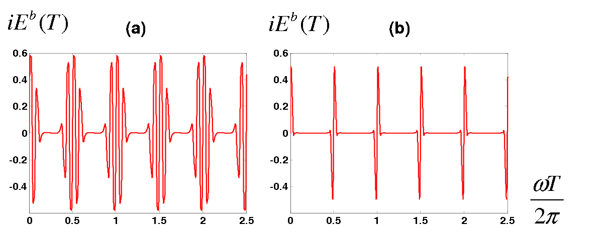
In Fig. 16 we plot examples of the atomic grating revivals. The trap frequency is chosen to be 0.14 times the recoil frequency , while the initial atomic phase-space distribution is tuned via temperature. Figure 16(a) corresponds to the atoms initially occupying the ground state of the harmonic trap only. Figure 16(b) corresponds to the initial condition of a thermal distribution with temperature equal to 50 times the recoil temperature. In both cases the trap frequency determines the period of the grating revival.
Complimentary to the proposal of using the echo shift [Eq. (29)] or recoil phase shift [Eq. (30)] to measure very weak harmonic perturbations in the last section, the revival of the atomic density grating predicted by Eq. (33) may be experimentally exploited to precisely determine the trapping frequency of tight traps.
IV Discussion and Summary
IV.1 Grating with general transmission functions
The discussion so far has been restricted to grating potentials using sinusoidal light shifts. In the following we shall discuss the generalization of the formula to include arbitrary grating transmission functions.
We shall first modify the light shift in Eq. (3) to include an imaginary part, e.g., , with . The imaginary part of the light shift potential could be due to the optical pumping effect of the light pulses Happer 1972 that act as an amplitude mask for atoms. More generally, the imaginary potential could also describe a particular harmonic component of an absorptive material grating Chapman et al. 1995. Following the principle of analytical continuation, Equation (8) and the scattering diagram in Fig. 2(b) can be modified to include this imaginary part as (Appendix A):
| (34) |
where
| (35) |
For a general amplitude/phase grating that has more than one spatial Fourier component in its transmission function, in Eq. (34) has to sum over contribution from all the Fourier components for the grating, e.g.,
| (36) |
where give the effective pulse area due to the order harmonic of the grating potential, and .
Notice here in Eqs. (34), (35), (36) and also in Eq. (8) the subindex is used to refer to the pulse in a TLI in Fig. 3, and can in fact be ignored for convenient reading.
To detect the resulting atomic density grating as the output of TLI, in this paper we have considered the method of a grating echo using Bragg scattering of a probe light, that is formulated in Eq. (5). Another detection method frequently used for matter gratings and for resonant standing wave masks is instead to monitor the overall transmission after an amplitude grating Clauser and Li 1994; Chapman et al. 1995; Fray et al. 2004; Turlapov et al. 2005; Tonyushkin and Sleator 2006. The formula developed in this work, e.g., Eq. (5) and Fig. 2(c) can be modified accordingly to (coherently) sum over the interaction with all the spatial harmonics of the transmission grating. We end up with the transmission signal given by [compare with Eq. (5)]:
| (37) |
where is the coefficient of the order spatial harmonic of the grating transmission function.
IV.2 Matter-wave coherence, displacement diagram and recoil diagram
In this work we discussed using Weyl functions to study the Talbot-Lau effect (in three dimensions) in free space and in a quadratic potential. We now come back to Eq. (1) to discuss the Weyl function as a measure of matter-wave coherence, and compare the “displacement diagram” technique here with the “recoil diagram” introduced by the authors of ref. Beach et al. 1982; Friedberg and Hartmann 1993 that has been widely used in the atom interferometry community AIBerman.
IV.2.1 Displacement diagram and conservation of matter-wave coherence
We come back to Eq. (1). As mentioned in the introduction, measures the overlap, or the second order field-correlation of matter-waves displaced in phase space by . As a particular example, measure the spatial coherence of a wavepacket before and after a particular displacement , which is also called the longitudinal coherence in matter-wave interferometry Klein et al. 1983. In Klein et al. 1983 it was pointed out that longitudinal coherence is conserved during free evolution, which is a fairly counterintuitive observation since wavepackets of atoms may expand a lot and one may suspect the coherence length of the wavepackets increases accordingly.
The conservation of during free evolution is only a particular example of Eq. (7), which more generally describes the conservation of matter-wave coherence that propagates in reciprocal phase space . In particular, momentum coherence of matter-waves given by is a Fourier component of atomic density grating (fringes), that propagates according to but with conserved magnitude. These propagating coherences reflect the correlation of matter-waves at different locations with different velocities, though they cannot be measured directly with any local measurement, except those on the axis . Equation (8) or (34) show how these phase space coherence can be manipulated with periodic potentials to create a revived momentum coherence for a local measurement.
Even more generally, it is easy to see from Eq. (1) the identity Chountasis and Vourdas 1998
| (38) |
which is equal to , the purity or linear entropy of matter-waves F. M. Cucchietti and Zurek 2003; Fano 1957. Matter-wave entropy is conserved in a non-dissipative/isolated potential, which may also be interpreted as a conservation of matter-wave coherence through the Weyl function, given by:
| (39) |
IV.2.2 Displacement diagram and recoil diagram

The recoil diagram was introduced by the authors of ref. Beach et al. 1982 together with a “Billiard Ball Model” of atom wavepackets to explain the photon echo phenomena, and also the Ramsey interference and two-photon echo in matter-wave interferometry Friedberg and Hartmann 1993. In a (x-t) recoil diagram such as Fig. 17(a), lines represent the trajectories of centers of wavepackets diffracted by optical pulses. The wavepackets are represented with “billiard balls” with a fixed radius equal to the coherence length of the wavepackets. Matter-wave interferes whenever two billiard balls cross each other. The visibility of the interfering fringe relies on the overlap of the billiard balls, while the fringe position is determined by the relative phase between the two wavepackets. A rigorous justification of using the “billiard ball model” is presented in Beach et al. 1982, which is related to the conclusion in ref. Klein et al. 1983 and also our previous discussion.
Examples of recoil diagrams due to a standing wave pulse (displacement diagram in Fig. 4), and for an “equal time 3-pulse” (displacement diagram in Fig. 8) grating echo interferometer is shown in Fig. 17 (a), (b) respectively. In contrast to the recoil diagram that concerns the coherence between individual pairs of wavepackets [such as the green path in Fig. 17(b)], the displacement diagram describes the overall coherence of the atomic sample, which is a sum of the coherence amplitudes between all pairs of the wavepackets with a same relative phase-space displacement. The displacement diagram is particularly convenient to describe the overall coherence of multiple diffraction orders, particularly when a sequence of multiple diffractions is considered (such as an N-pulse sequence given by Fig. 3). The overall coherence of an atomic sample is directly related to interference readouts in most interferometry setups where the interference fringes are retrieved across the whole atomic sample.
IV.2.3 Dephasing and decoherence
Finally, it is instructive to consider the dephasing effect in both the recoil diagram picture and in the displacement diagram picture. For a matter-wave interferometer perturbed by an external potential, the phase of wavepackets may be in-homogeneously broadened that reduce the overall coherences of matter-waves and thus the fringe contrast. This is referred to as a dephasing effect. Dephasing effects can be described by a recoil diagram, by assigning each “billiard ball’ with a different phase and by varying the “radius of the billiard ball” to account for wavepacket distortions.
In the displacement diagram picture, the dephasing effect broadens and shifts the Weyl function distribution in the reciprocal phase space, for example, the dephasing effect due to a quadratic potential corresponds to a shift of Weyl function described by Eq. (27). However, any broadenings or shifts of Weyl function distribution need to obey the conservation law given by Eq. (39). In contrast, the reduction of interferometer fringe visibility accompanied by a violation of Eq. (39) is due to a loss of information or an increase of entropy in the matter-wave system, and should be referred to as decoherence effects Kokorowski 2001; foot:exp4.
IV.3 Summary and conclusion
We have generally discussed a vector theory of Talbot-Lau effects due to N standing wave pulses by considering an N-pulse grating echo interferometry configuration (Fig. 1). A displacement diagram (Figs. 2 and 10) is introduced to calculate the grating echo diagrammatically. To illustrate the convenience of the diagrammatic technique, we discuss examples of TLI that are related to recent experiments Su et al.; Wu et al. 2007; Wu et al., in particular, we discuss an example TLI with standing wave k-vector span two dimensions. We study the dephasing of these TLI schemes due to harmonic confinements (Table 1), and predict the echo shift [Eq. (29)] and the recoil phase shift [Eq. (30)] that have been observed experimentally Wu 2007. These effects should be useful to measure the curvature of an atomic potential. The displacement diagram method is further extended to include a pulsed harmonic trap [Eq. (31)] and we discuss a time-domain version of the original Lau effect [Eq. (32)]. Using the displacement diagram in a tightly confined trap, we give the expression of the atomic density grating revivals [Eq. (33)]. The formula introduced in this work can be extended to describe TLE due to diffraction gratings with general grating transmission functions. Application of Weyl functions in this work has been restricted to Talbot-Lau effects involving multiple diffraction orders from diffractive gratings. But the method is generalizable to other interferometry configurations with fewer interfering paths.
Coherences, or “off-diagonal terms of a density matrix” Fano 1957, have a clear definition in discrete systems but not so clear for matter-waves that have a continuous spectrum Baudon et al. 1999. In the last part of this work we have briefly discussed Weyl function as a convenient measure of matter-wave coherence. Weyl function as a phase-space correlation function measures the overlap of matter-waves before and after a phase-space displacement. Similar to the definition of the Wigner function, Equation (1) involves a Fourier transform of off-diagonal part of a density matrix. The Fourier transform removes the ambiguity due to the ill-defined off-diagonal terms, while keeping all the physical information of matter-wave coherences foot:exp5. We thus suggest using Weyl function to define matter-wave coherence and more generally to define coherences in system with a continuous spectrum. We suggest that according to this definition, a conservation law of matter-wave coherence [Eq. (39)] that directly link to the matte-wave entropy can unambiguously distinguishes decoherence and dephasing effects. Practically, it seems that to consider the Weyl function or the displacement operator, instead of considering the evolution of particular matter-wave states, is more convenient for elucidating the dynamics of matter-wave coherences during a particular interferometric observation.
Acknowledgements.
We thank Dr. A. Tonyushkin for careful reading and helpful suggestions to the manuscript of this paper.Appendix A Propagation properties of the displacement operator
We consider the evolution of the displacement operator in the Heisenberg picture. Notice that can also be expressed as .
We consider three type of propagators:
| (A-1) |
We have, during free propagation in an accelerating frame with acceleration constant ,
| (A-2) |
In a harmonic trap:
| (A-3) |
Transformation of under a standing wave pulse is given by:
| (A-4) |
Finally, we consider the propagator due to a standing wave pulse with complex area:
| (A-5) |
The transformation of is given by:
| (A-6) |
In Eq. (A-6) is the modified Bessel function of the first kind. From Eq. (A-6) to Eq. (34) we use the Graf summation formula for Bessel functions with complex arguments Wang and Guo 1997. The multiple-valued arguments of Bessel functions in Eq. (34) is chosen to be single valued according to Wang and Guo 1997.
References
- Balazs and Jennings (1984) N. L. Balazs and B. K. Jennings, Phys. Rep. 104 (1984).
- Heller (1976) E. J. Heller, J. Chem. Phys. 65, 1289 (1976).
- Berry (1977) M. V. Berry, Phil. Trans. R. Soc. A 287 (1977).
- Smithey et al. (1993) D. T. Smithey, M. Beck, M. G. Raymer, and A. Faridani, Phys. Rev. Lett. 70, 1244 (1993).
- Bishop and Vourdas (1994) R. F. Bishop and A. Vourdas, Phys. Rev. A 50, 4488 (1994).
- Vourdas (2006) A. Vourdas, J. Phys. A 39, 65 (2006).
- Chountasis and Vourdas (1998) S. Chountasis and A. Vourdas, Phys. Rev. A 58, 848 (1998).
- (8) E. J. Su, S. Wu, and M. G. Prentiss, physics/0701018.
- Wu et al. (2007) S. Wu, E. J. Su, and M. G. Prentiss, Phys. Rev. Lett. 99, 173201 (2007).
- Wu (2007) S. Wu, Ph.D. thesis, Harvard Univ. (2007).
- Pfeiffer et al. (2006) F. Pfeiffer, T. Weitkamp, O. Bunk, and D. C., Nature Physics 2, 258 (2006).
- Talbot (1836) H. Talbot, Phil. Mag. 9, 401 (1836).
- Berry (1996) M. Berry, J. Mod. Optics 43, 2139 (1996).
- Lau (1948) E. Lau, Annalen Der Physik 2, 417 (1948).
- Jahns and Lohmann (1979) J. Jahns and A. Lohmann, Opt. Comm. 28, 263 (1979).
- Chapman et al. (1995) M. S. Chapman, C. R. Ekstrom, T. D. Hammond, J. Schmiedmayer, B. E. Tannian, S. Wehinger, and D. E. Pritchard, Phys. Rev. A 51, R14 (1995).
- Deng et al. (1999) L. Deng, E. W. Hagley, J. Denschlag, J. E. Simsarian, M. Edwards, C. W. Clark, K. Helmerson, S. L. Rolston, and W. D. Phillips, Phys. Rev. Lett. 83, 5407 (1999).
- Clauser and Li (1994) J. F. Clauser and S. Li, Phys. Rev. A 49, R2213 (1994).
- (19) Atom interferometry, edited by P. R. Berman (Academic Press, Cambridge, 1997).
- Brezger et al. (2002a) B. Brezger, L. Hackermüller, S. Uttenthaler, J. Petschinka, M. Arndt, and A. Zeilinger, Phys. Rev. Lett. 88, 100404 (2002a).
- Hackermuller et al. (2003a) L. Hackermuller, S. Uttenthaler, K. Hornberger, E. Reiger, B. Brezger, A. Zeilinger, and M. Arndt, Phys. Rev. Lett. 91, 90408 (2003a).
- Hackermuller et al. (2003b) L. Hackermuller, K. Hornberger, B. Brezger, A. Zeilinger, and M. Arndt, Appl. Phys. B 77, 781 (2003b).
- Hornberger et al. (2005) K. Hornberger, L. Hackermuller, and M. Arndt, Phys. Rev. A. 71, 023601 (2005).
- Berninger et al. (2007) M. Berninger, S. A., D. S., and A. M., Phys. Rev. A. 76, 013607 (2007).
- Fray et al. (2004) S. Fray, C. A. Diez, T. W. Hänsch, and M. Weitz, Phys. Rev. Lett. 93, 240404 (2004).
- Cahn et al. (1997) S. B. Cahn, A. Kumarakrishnan, U. Shim, T. Sleator, P. R. Berman, and B. Dubetsky, Phys. Rev. Lett. 79, 784 (1997).
- Weel et al. (2006) M. Weel, I. Chan, S. Beattir, A. Kumarakrishnan, D. Gosset, and I. Yavin, Phys. Rev. A 73, 63624 (2006).
- Mossberg et al. (1979) T. W. Mossberg, R. Kachru, E. Whittaker, and S. R. Hartmann, Phys. Rev. Lett. 43, 851 (1979).
- Strekalov et al. (2002) D. Strekalov, A. Turlapov, A. Kumarakrishnan, and T. Sleator, Phys. Rev. A 66, 23601 (2002).
- Turlapov et al. (2005) A. Turlapov, A. Tonyushkin, and T. Sleator, Phys. Rev. A 71, 043612 (2005).
- Tonyushkin and Sleator (2006) A. Tonyushkin and T. Sleator, Phys. Rev. A 74, 053615 (2006).
- Carnal et al. (1995) O. Carnal, Q. Turchette, and H. Kimble, Phys. Rev. A 51, 3097 (1995).
- Brezger et al. (2002b) B. Brezger, M. Arndt, and A. Zeilinger, J. Opt. B: Quantum Semiclass. Opt. 5, 82 (2002b).
- Clauser and Reinsch (1992) J. F. Clauser and M. W. Reinsch, Appl. Phys. B 54, 380 (1992).
- Dubetsky and Berman (1999) B. Dubetsky and P. R. Berman, Phys. Rev. A 59, 2269 (1999).
- Beach et al. (1982) R. Beach, S. R. Hartmann, and R. Friedberg, Phys. Rev. A 25, 2658 (1982).
- Happer and Mathur (1967) W. Happer and B. S. Mathur, Phys. Rev. 163, 12 (1967).
- Gupta et al. (2002) S. Gupta, K. Dieckmann, Z. Hadzibabic, and D. E. Pritchard, Phys. Rev. Lett. 89, 140401 (2002).
- (39) S. Wu, E. J. Su, and M. G. Prentiss, in preparations.
- (40) Though a 3D plot as those in Fig. 9(a) is necessary for a 2D displacement diagram, practically we may simply use the projection plot similar to Fig. 9(c).
- Bertoldi et al. (2006) A. Bertoldi, G. Lamporesi, L. Cacciapuoti, M. de Angelis, M. Fattori, T. Petelski, A. Peters, M. Prevedelli, J. Stuhler, and G. M. Tino, Eur. Phys. J. D 40, 271 (2006).
- McGuirk et al. (2002) J. McGuirk, G. Foster, J. Fixler, M. Snaden, and M. A. Kasevich, Phys. Rev. A 65, 33608 (2002).
- Peters et al. (2001) A. Peters, K. Chung, and S. Chu, Metrologia 38, 25 (2001).
- (44) Similar effect was discussed in Peters et al. 2001 for a Ramsey-Bordé type interferometer under a gravity gradient.
- (45) A more thorough discussion on the echo profile shift and recoil phase shift, including an experimental study using interferometry with magnetically guided atoms, can be found in Wu 2007.
- Happer (1972) W. Happer, Rev. Mod. Phys. 44, 169 (1972).
- Friedberg and Hartmann (1993) R. Friedberg and S. Hartmann, Phys. Rev. A 48, 1446 (1993).
- Klein et al. (1983) A. G. Klein, G. I. Opat, and W. A. Hamilton, Phys. Rev. Lett. 50, 563 (1983).
- F. M. Cucchietti and Zurek (2003) J. P. P. F. M. Cucchietti, D. A. R. Dalvit and W. H. Zurek, Phys. Rev. Lett. 91, 210403 (2003).
- Fano (1957) U. Fano, Rev. Mod. Phys. 29, 74 (1957).
- Kokorowski (2001) D. A. Kokorowski, Ph.D. thesis, M. I. T. (2001).
- (52) The loss of knowledge to the system may be regained through a measurement. The process shall still be referred to as a decoherence effect, as Equation (39) has to be violated during such measurement processes.
- (53) We notice the closely-related concepts in coherent light optics, such as in the book by Mandel L. and Wolf E., Optical Coherence and Quantum Optics, Cambridge University Press.
- Baudon et al. (1999) J. Baudon, R. Mathevet, and J. Robert, J. Phys. B 32, 173 (1999).
- Wang and Guo (1997) Z. X. Wang and D. R. Guo, Introduction to special functions (Peking Univ. Press, 1997).