A random walk approach to anomalous particle and energy transportPreprint: ….
Abstract
The combined Continuous Time Random Walk (CTRW) in position and momentum space is introduced, in the form of two coupled integral equations that describe the evolution of the probability distribution for finding a particle at a certain position and with a certain momentum as a function of time. The integral equations are solved numerically with a pseudospectral method that is based on the expansion of the unknown functions in terms of Chebyshev polynomials. In parallel, Monte-Carlo simulation are performed. Through the inclusion of momentum space, the combined CTRW is able to yield results on density and temperature profile evolution, on particle and heat fluxes and diffusivities, and on kinetic energy distributions. Depending on the choice of the probability distributions of the particle displacements in position and momentum space, the combined CTRW is non-local in position-space, in momentum-space, and in time (non-Markovian), and it is able to model phenomena of anomalous transport in position as well as in momentum (or energy or velocity) space. An application is made to a toroidally confined plasma that undergoes off-center injection of cold plasma (off-axis fueling), using two variants of the model, the mixed model and the critical gradient model. The phenomenon of profile stiffness is addressed, and it is shown that it can be reproduced by the combined CTRW with varying success, both for the density and for the temperature profile, respectively. The particle and energy confinement times are determined, and their dependence on the applied intensity of plasma heating is discussed. Finally, the analysis of the particle and heat fluxes shows that the dynamics realized in the combined CTRW is incompatible with the classical approach of Fick’s or Fourier’s law for particle and heat transport, respectively, so that particle and heat diffusivities determined through the latter are not an adequate characterization of the actual transport process in position and momentum space.
Keywords:
random walks; Levy-walks; fractals; turbulence; anomalous diffusionpacs
05.40.Fb, 05.65.+b, 47.53.+n, 52.25.FiI Introduction
Anomalous transport phenomena are conveniently characterized by the scaling of the mean square displacement of an ensemble of particles with time . Often, a power-law scaling is observed,
| (1) |
where the characteristic index is used to discern normal or classical diffusion with from anomalous diffusion with , and in particular sub-diffusion for and super-diffusion for . Continuous time random walk (CTRW), introduced in Montroll65, has successfully been applied to model various phenomena of anomalous transport, including sub- and super-diffusive phenomena, in the fields of physics, chemistry, astronomy, biology, and economics (see e.g. the references in Metzler00).
Most applications of the CTRW in physics model the random walk of particles in position space. Two variants of CTRW are used, the waiting or trapping model, introduced by Montroll65, and the velocity model, introduced by Shlesinger87. The two models differ in the timing of the random walk. In both models, the random walker (particle) takes steps of random size and/or direction in position space. In the trapping model, the random walker waits for a random time at the location it was brought to by its last step before it moves a new step away, in the step itself no time is consumed. In the velocity model, a particle is constantly moving, and the travel time, the time it takes a particle to complete its spatial step, determines the timing. To determine the travel time, a velocity has to be assumed, and since velocity space dynamics usually was not taken into account so-far, this velocity was usually assumed to be constant and for convenience set equal to one.
The main purpose of this article is to extend the position space CTRW in the variant of the velocity model, and to include also momentum space dynamics, so that the velocity does not play anymore just a dummy role, but reflects the dynamics that take place in velocity (or momentum) space, in parallel with the position space evolution. This extension to the combined CTRW in position and momentum space is relevant in applications to turbulent fluids, and, most prominently, in applications to turbulent laboratory and astrophysical plasmas, where localized turbulent electric fields, magnetic field discontinuities (e.g. at magnetic reconnection sites), externally or internally generated waves or other forms of induced plasma heating, etc., are the cause of a highly dynamic evolution in momentum space. The combined CTRW in such applications is able to yield information about kinetic energy distributions, temperature profiles, heat fluxes, and heat diffusivities, together of course with information about particle densities, particle fluxes, and particle diffusivities.
The CTRW formalism was first applied to plasmas by Ref. Balescu95, and it was shown that in the form of the critical gradient model (vanMil04, vanMil04b), the CTRW can successfully model various observed phenomena of anomalous transport in confined turbulent plasmas, where though so-far only the evolution in position space was taken into account. In Vlahos04, we performed a Monte Carlo simulation study of the combined CTRW in position and momentum space, in application to the plasma in the solar corona, where the main physical interest was in modeling the appearance of non-thermal energy distributions and the related electromagnetic emission spectra during solar flares. In this article, we introduce a set of equations that describe the combined CTRW in position and momentum space, and we present a method for solving them numerically.
In order to illustrate the capabilities of the combined CTRW and to demonstrate the importance of the inclusion of momentum space in the random walk approach, we present an application to laboratory plasmas, confined in toroidal devices such as the tokamak. Toroidally confined plasmas exhibit a variety of anomalous transport phenomena, both what particle and heat transport are concerned, respectively, and which clearly contradict what classical diffusion would predict. In view of the intended application, we just mention a few manifestations of anomalous transport in confined plasmas: (i) Measured diffusion coefficients (for particle and for heat diffusion) are usually larger than the neoclassical values, i.e. those derived from collisional effects in toroidal geometry (e.g. Garbet04). (ii) A characteristic property in confined plasmas is profile stiffness (also termed resilience or consistency), which denotes the preference of a plasma to stay close to a certain density and temperature profile (in direction of the minor radius of the toroidal confinement device), i.e. the profiles are usually peaked at the center, and they are to a large degree unaffected by the way the plasma is distorted externally, e.g. through the localized off-center injection of particles or heat. Profile stiffness is an anomalous transport phenomenon in the sense that particles or energy are transported ’up-hill’, against the density or temperature gradient, respectively, which, in the case of normal diffusion, would drive diffusion ’down-hill’. Profile stiffness is discussed e.g. in Ref. Garbet04, and examples of related experiments include Luce92, Petty94, Ryter03 and are reviewed e.g. in Ryter01. (iii) The experimental analysis in Ref. Lemoine05 finds that plasma diffusion is characterized by particle displacements that can be characterized statistically with a probability distribution that exhibits a power-law tail with a power-law index 2. This implies that particles undergo occasionally large displacements, so that the spatial diffusion process can be non-local in nature. (iv) Ref. Hoang01 and, similarly, Ref. Baker01 infer from experiments that the electron heat transport is threshold dependent, in the sense that transport is activated only if the temperature gradient exceeds a certain threshold, . We just note that the properties (ii) and (iv) are very reminiscent of Self-Organized Criticality (SOC; Bak87).
Based on these experimental results, the application we present is to an experiment where a colder plasma is injected localized off the center (off-axis fueling), and we will focus on phenomena of density and temperature profile stiffness, the quality of the particle and the energy confinement, and the possibility to characterize transport with particle and heat diffusivities. In accordance with the mentioned experimental result (iii), particle displacements in position space will partly be allowed to be large, i.e. of system size, so that position space transport will throughout be of partly non-local nature. To explore the influence of the momentum space evolution on the over-all dynamics, we will in all applications consider two cases for displacements in momentum space, namely small displacements that correspond to a very low level of energy injection (heating) into the system and to classical random walk in momentum space, and large displacements in momentum that follow a power-law distribution, and which represent the case of intense heating and non-local transport in momentum space.
In Sec. II, the equations for the combined CTRW in position and momentum space are introduced, first in a general three dimensional form and then in a one dimensional version that will be used in the applications. Also, short explanations on Monte-Carlo simulations are given, and the pseudospectral method based on Chebyshev polynomials, with which the combined CTRW equations are solved numerically, is shortly presented. Sec. III contains the applications to the off-center plasma injection experiment. In order to specify the combined CTRW to the set-up of a toroidally confined plasma, two models will be introduced, the mixed model and the critical gradient model, which realizes the mentioned experimental feature (iv). In Sec. IV, the particle and heat confinement times, fluxes and diffusivities are discussed. Finally, Sec. V presents a summary and the conclusions, and a more detailed presentation of the pseudospectral numerical method is given in App. A.
II Continuous Time Random Walk in position and momentum space
II.1 The distribution of increments
In the random walk approach, the different processes a particle can undergo in its evolution are formally separated, and for the random walk of a particle in a turbulent plasma they consist in (i) collision and heating or acceleration events, in which mainly the momentum and much less the position of a particle changes, and which include particle-particle collisions, particle-wave collisions, absorption of electromagnetic waves, interaction with localized, turbulent electric fields; (ii) trapping events, mostly in inhomogeneous magnetic field structure, and in which neither position nor momentum of a particle is changed; and (iii) free travel or drift events events, during which the energy of a particle remains unchanged. In each of these events, a particle spends a certain time.
For simplicity, we will throughout the following omit the trapping events, and we only consider acceleration and free travel events. Moreover, we take into account only the time spent in the free travels, the acceleration time is considered negligible and neglected. We note that the free flight times provide a basic coupling between momentum and position space dynamics, since the acceleration events have a direct influence on the velocity of a particle, and the latter in turn determines, together with the travel distance, the free flight time and thus the overall timing of the random walk. (If one alternatively would take into account only the trapping times, then the dynamics in position and momentum space would be decoupled, unless the trapping time would depend in some way on momentum and position.)
The basic quantity for the random walk is the probability density function (pdf) of random walk increments or steps, which determines the probability for a particle to perform a jump in momentum space (corresponding to heating, acceleration, or possibly also dissipation), to freely travel a directed distance in position space, and to spend on this free travel a time . The free travel time is defined as , with the jump-length and the instantaneous velocity , which is a direct function of the instantaneous momentum . We assume and to be independent random variables, with pdf and , respectively, so that the joint pdf decouples to
| (2) | |||||
where the conditional probability for the free flight time, given the length of the step and the particle’s velocity, can be written as , so that the pdf of increments takes the form
| (3) | |||||
We just note that a different choice for the delta function seems to be , with this choice though, the joint pdf would have wrong units, and also the marginal distributions calculated from it would be inconsistent.
II.2 The pdf of the turning-points
In the derivation of the equations for the combined CTRW equations in position and momentum space, we follow the formalism of e.g. Zumofen93 for the CTRW equations in position space alone, which we extend by adding momentum. The basic CTRW equations in Zumofen93 are a set of two integral equations that express the conservation of particles in integral form. Here, we use the variant of the velocity model, since we want to take the free flight times explicitly into account,
Following Zumofen93, we introduce the concept of turning points, at which a particle takes a new step in its random walk. More precisely, as turning points of the random walk we define the points in position () and momentum () space where the particles arrive at and undergo an acceleration event. Two turning-points are thus separated by an acceleration event and a free jump in position-space, and we are in principle free to choose in which order the two processes happen, for practical reasons though we let the cycle start with an acceleration event. We define as the distribution of the turning points, which describes the rate at which particles arrive at time at the turning point that is located at (as a rate has units ). Adding the momentum to the evolution equation for in Zumofen93 and using the distribution of increments of Eq. (3) yields
| (4) | |||||
The first term on the right hand side just describes a completed cycle of a CTRW step in position space, momentum space, and time: in order to arrive at a turning point at at time , a particle must have arrived at a turning point at an earlier time , where after it has performed a step in momentum space and then a step in position space, for which the particle has spent a time that must equal the free flight time, . Since we assume the free flight to take place after the acceleration event, the momentum during the free flight is , so that (if we would assume the free flight to take place before the acceleration event, then the free flight time would depend on , and the integrals would become more complicated in their formal structure). The limits of the integration are imposed by causality, we cannot consider at time spatial increments that have free flight times larger than . The second term on the right hand side of Eq. (4) takes the initial conditions into account, is the particle distribution at time . Finally, in Eq. (4) is a source term that represents a continuous particle source (more precisely, is the source rate, with units ). Writing the source in this form implies that particles are injected at turning points, which means that injected particles are immediately accelerated after their injection.
We just note that if also trapping and acceleration times were taken into account, then two more temporal integrals would have to be added to the equation, which is formally possible, it increases though the numerical complexity, computing time would be increased in the numerical solution, and good numerical precision would be more difficult to be achieved.
II.3 The propagator
The propagator is defined as the probability distribution for a particle to be at time at position anywhere at a turning point or in-between two turning points (the units of are ). The propagator evolution equation is again determined by generalizing the corresponding equation in Zumofen93 to include also momentum,
| (5) | |||||
The limits of the spatial integral express again the fact that particles cannot travel spatial distances at time that take flight times longer than . is the probability for a particle to be found at a certain spatial location on its free travel in-between two turning-points, which equals the probability to make a spatial jump in the direction of , with length at least and of duration at least , being though at time exactly at position . In spherical coordinates with , and where the angles and determine the direction of a jump and is its length, can be expressed as (see the explanations below)
| (6) | |||||
where and . Note the form of the first delta function, in contrast to the conditional pdf for the free flight times — the seemingly alternative choice would cause to have wrong units, i.e. instead of the needed .
Eq. (5) states that a particle is at position at time if it was at a turning point at time , it underwent an acceleration event which changed its momentum by , and it is now on a free flight event whose duration is at least , being though at time exactly at position . Since no time is assumed to be consumed in the acceleration events, we cannot locate the particles during acceleration events, but only during the free flights in position space. Again, the assumption that the turning points are the points where a particle starts undergoing first an acceleration event, and the acceleration event is then followed by a free flight event, was used in the formulation of Eq. (5).
II.3.1 Explanations on the form of
In spherical coordinates , the probability (not the density) to make a jump of length into the direction and in time is given by multiplying Eq. (3) by the differentials of the coordinates,
| (7) |
and the probability to make a jump in the direction larger than and is
| (8) |
We furthermore demand that the walker has traveled a distance exactly at time into the fixed direction , i.e. , which is conveniently enforced through a delta function, (the variant has wrong units, see the remark above). In spherical coordinates, the delta function is of the form
| (9) |
(e.g. Jackson62), of which we need the spatial part only, since the direction is explicitly kept fixed, so that the condition must be written as
| (10) |
Combining Eqs. (8) and (10) leads to Eq. (6), whereby the angular differential in Eqs. (8) is understood as part of in Eq. (6).
II.3.2 Marginal distribution
Once the propagator is determined, the particle density distribution and the momentum distribution function are given as marginal distributions of ,
| (11) |
and
| (12) |
respectively. For the kinetic energy distribution , we first define the distribution of ,
| (13) |
The distribution of is then found from the distribution of through the relation , or . From the expression for the total energy in terms of the momentum, , and the definition of the kinetic energy, , it follows that , where is the particle mass and the speed of light.
Defining the temperature as the mean kinetic energy per particle, , with the Boltzmann constant, we can determine the temperature profile as
| (14) |
with and .
II.4 Remarks on possible reformulating of the equations
The explicit appearance of the time, position, and momentum in the integration limits of Eqs. (4) and (5) make the straightforward application of Fourier and Laplace transforms with the corresponding convolution theorems impossible. As a consequence, the equations cannot trivially be reformulated into one equation for the propagator alone, and also a transformation to a different type of equation (integro-differential or possibly fractional diffusion equation) seems at least difficult.
Also direct ways of reformulating into one equation do not work, e.g. when inserting into and trying to change the order of the integrations to identify under the outer integrals, it turns out that the free flight delta function does not allow the change of the order of integrations because of appearance of the velocity , which is a function of .
II.5 The 1-dimensional case
We specify the general equations to the 1-dimensional form, using the variables for position and for momentum, and, in view of the intended application, we assume the system to be finite in -direction, , with half the system size. The turning point equation [Eq. (4)] in one dimension takes the form
| (15) | |||||
The spatial integration limits are equivalent to the condition from Eq. (4), and moreover they restrict to to account for the finiteness of the system.
In one dimension, the propagator equation [Eq. (5)] becomes
| (16) | |||||
The spatial integration limits are the same as for in Eq. (15).
For , the probability for a particle to make a spatial jump of length at least in the direction and of duration at least , being though at time exactly at position [see Eq. (6)], there are two choices of interest. First, can be independent of the direction of , and the jump direction is given by the pdf of increments , which is two-sided and includes the sign of , so that can be written as
| (17) | |||||
This form of is adequate for magnetized plasmas, where particles cannot travel along straight lines in the direction of their velocity. The factor appears since we consider the symmetric two-sided distribution , with positive and negative arguments: should express the probability to make a jump larger than in the direction of , which is half of the probability to make a jump larger than to either side for a two-sided distribution of increments that is assumed to be symmetric.
Second, the jump might be in the direction of the instantaneous velocity, i.e. along . In this case, we consider a one-sided pdf of increments only for the length of the jump, and we define as
| (18) | |||||
In this case, everywhere is understood, i.e. also in the expressions for and , Eqs. (15) and (16), respectively. This form of is adequate for particles in free space or in an unmagnetized plasma, where the particles travel along straight lines in the direction of their velocity. This form is also useful in the case where the velocities do not represent the thermal velocities, but e.g. the set of possible drift velocities in a magnetized plasma. No factor appears in Eq. (18), since the one-sided distribution of increments is considered.
II.6 The final equations
To calculate the -integral in the expression for , Eq. (15), we note that the delta function implies that , as long as is in the -integration range, which is obviously the case if . If , then this condition reduces to , and if then it must hold that , which are just the conditions imposed by the integration limits of the -integral. In the case where the upper integration limit is , it again holds that , and the like if the lower integration limit is . It thus follows that the equation for writes as
| (19) | |||||
Also in any of the two cases of Eqs. (17) and (18) for , the temporal integral is trivial, as long as is in the integration range of the integral, i.e. if . This is always the case, since the lower limit of the -integration implies that and the delta function in front of the integrals ensures the relation , so that the inequality follows. Eq. (17) thus turns to
| (20) | |||||
and Eq. (18) becomes
| (21) | |||||
In the applications presented below, we will use the variant for the case of a magnetized plasma, we thus insert from Eq. (20) into the expression for [Eq. (16)], which yields
| (22) | |||||
On doing the -integration, the delta function would impose that , if this is contained in the -integration range. Obviously, , since a positive term is subtracted from . On the other hand, if , which is though exactly the condition imposed by the -integration limits. The integration is thus trivial and can be done e.g. by substituting , which yields
| (23) | |||||
Last, we introduce the abbreviation
| (24) |
so that the propagator equation takes the final form
| (25) | |||||
The marginal distributions for the density and the momentum, as well as the kinetic energy distribution and the temperature profile are determined completely analogous to the way described in Sec. II.3.2, for the case of here only one spatial and one momentum coordinate. The only modification we make is that the one-dimensional version of the relation of the temperature to the mean kinetic energy is used, .
II.7 Connection to electric fields
In a plasma, acceleration events are usually connected to the appearance of electric fields, and we consider the increments in momentum to be caused by electric fields, assuming that
| (26) |
with the particle charge, the electric field, and an acceleration time assumed to be constant (in this way, the statistics of the duration of the acceleration process is absorbed in the statistics of the effective electric field). Since must hold, the connection of the pdf of to the pdf of the electric fields is given by
| (27) |
II.8 Numerical solution of the CTRW equations
We solve the system of Eqs. (19) and (25) numerically with a pseudospectral method based on Chebyshev polynomials. In this method, the unknown functions and are expanded in terms of Chebyshev polynomials in the -, -, and -direction, and in case where the integral equations are linear (which basically implies that the distributions of increments and do not contain information on ), the integral equations turn into a system of linear algebraic equations, which can be solved with a standard linear system solver. In App. A, a more detailed description of the numerical method is given.
The critical gradient model, which will be introduced below (Sect. III.2.2), is non-linear, the spatial jump increments contain information on the density gradient, so that in principle the pseudospectral method is applicable also to this case, it yields though a system of non-linear algebraic equations, for which we have not yet implemented a numerical method to solve it (see the more technical explanations in App. A), so that the results presented here for the critical gradient model are all derived with Monte Carlo simulations.
II.9 Monte Carlo simulations
In parallel to the numerical solution of the CTRW equations, Monte Carlo simulations are performed, in two different versions. In the first version, an individual particle has no information during its evolution on the rest of the particles. This version is very fast in what computing time is concerned, and it is used to verify results of the mixed model (introduced in Sect. III.2.1) and to determine the mean velocity profile in Sect. IV.2. In the second version, an individual particle knows where all the other particles are during its evolution, and it is influenced by local statistical properties, such as the density gradient. This version has to be used for the critical gradient model (introduced in Sect. III.2.2), and it is very demanding in computing time, so that statistically sensitive quantities such as the mean velocity profile, and therewith the particle and heat flux (see Sect. IV.2), could not be determined reliably enough and are not presented in this article.
III Application
III.1 overview
We consider a plasma in a toroidal confinement device such as a tokamak, and our purpose is to study the particle and heat transport phenomena in the direction of the minor radius of the torus, perpendicular to the confining magnetic field. This direction is of major interest in tokamaks, since heat or particle losses in this direction determine the quality of the achieved confinement.
III.2 Parameters and distribution of increments
We assume a finite spatial range , with cm. For numerical reasons, we have to truncate also momentum space, we usually assume the largest positive momentum to be , except in the case of pure power-law increments in , where we use , with the thermal momentum. In all applications below, the system initially is empty, , there is only a source term active that is constant in time. The momentum distribution of the particles at injection into the system is throughout a Gaussian distribution, with plasma temperature keV for the uniform background source, so that g cm/s (cm/s) for electrons.
The distribution of increments we use below are a combination of two basic distributions, one which allows only small increments compared to the system size, and one which allows also large increments, of the order of system size or even larger. For the former, a natural choice are Gaussian distributions,
| (28) |
for position increments, and
| (29) |
for momentum increments, and we usually use cm, and g cm/s, respectively.
As distribution for large increments, we use Levy-like distributions with power-law tails,
| (30) |
in position space, with cm and a standard value for the power-law index , as it corresponds to a random walk through a fractal environment with fractal dimension (in 3-D space, , see Isliker03). In momentum space, we analogously choose
| (31) |
with and power-law index , chosen such that there is not unrealistically strong heating of the plasma.
We just note that for the purpose of studying non-local effects on transport, one could, instead of power-law distributed increments, also apply Gaussian distributed increments that are large, where large is understood in the sense of being comparable to the system-size.
The CTRW approach has the possibility to model a wide variety of anomalous transport phenomena, whose concrete form is determined by the the choice of the distributions of increments. In order the random walk model to become relevant for toroidally confined plasmas, the increment distributions must incorporate some essential properties of the physical system. Here, we make two different choices for the distribution of position increments.
III.2.1 The mixed model
First, we implement the observation that anomalous diffusion is more active to-wards the edges of the plasma, whereas the center exhibits more normal diffusive behaviour, the plasma is better confined near the center (see the remark in the following Sec. III.2.2). We thus let in the mixed model the distribution of position increments be spatially dependent on such that it is a weighted mixture of a power-law and a Gaussian distribution,
| (32) | |||||
The function equals one in the center and falls off linearly to-wards the edges,
| (33) |
where we use the basically arbitrary values cm and , which are chosen by trial and error in order to achieve a good confinement of the particles in the system.

,
III.2.2 The critical gradient model
In the second choice for the distribution of position increments we follow the critical gradient model, suggested originally by Imbeau01 (see also Garbet04b) in the frame of classical diffusion (Fick’s or Fourier’s law), making the basic assumption that the heat (particle) diffusivity depends critically on the density or temperature gradient, in the sense that transport becomes efficient only if the respective gradient exceeds a threshold. A variant of the critical gradient model was implemented in the frame of CTRW by vanMil04, vanMil04b, with the distribution of position increments depending on the local density gradient. We thus set
| (34) |
with the particle density and the threshold, so that the distribution of increments is a power-law in regions where a large density gradient has developed, and it is Gaussian in regions where the gradients are small.
Remarks: (i) The general CTRW formalism we introduced would also allow to use different criticality conditions, the distribution of position increments could e.g. be made critically dependent on the temperature gradient, or on a combination of the density and the temperature gradient, and also in the distribution of momentum increments a critical dependence could be introduced. (ii) The critical gradient model in Refs. vanMil04, vanMil04b is different from the critical gradient model used here in that waiting times and not free flight times are used in Refs. vanMil04, vanMil04b, which moreover are assumed to always follow an exponential distribution, and of course momentum space is not included. (iii) For symmetry reasons, one would expect that in the critical gradient model the density gradient is small at the center and becomes larger to-wards the edges, so that transport is more normal near the center and more anomalous to-wards the edges, which is just the scenario we explicitly implement in the mixed model. (iv) The density gradient dependence of the position increments introduces a non-linearity into the integral equations of the CTRW, whereas the equations of the mixed model are linear in .
III.2.3 The momentum increments
As distribution of momentum increments we use either a pure Gaussian distribution or a pure power-law distribution. These two cases correspond to low and high level activity (heating) in momentum space, respectively, and they allow us to explore the role of momentum space dynamics for the system evolution in the two extreme cases of interest, the almost local and the non-local momentum transport, respectively.
III.3 Uniform injection in space and time

In the first application, we consider the case where the plasma is uniformly and continuously injected into the system, with the initial position and injection time of the particles uniformly distributed in the spatial interval and in the time interval , respectively, with the final time up to which the system is monitored. The initial momentum follows a thermal distribution with a fixed temperature of keV. The source function thus takes the form
| (35) |
with , the thermal momentum.
In Fig. 1, the density profiles as a function of time, normalized to the total number of injected particles , are shown for the mixed model with Gaussian and power-law distributed increments in momentum, respectively. The initial density is zero, according to the chosen set-up, and the system evolves to a stationary dynamic equilibrium state. Fig. 2 shows the density profiles at the final time , including now also the critical gradient model with again Gaussian and power-law distributed momentum increments, respectively. In the cases of the mixed model and the critical gradient model with Gaussian momentum increments, density profiles are formed that are peaked at the center — within the statistical error for the critical gradient model —, with the characteristic difference that in the mixed model the density profile has flatter wings to-wards the edges, the particles are more concentrated at the center. The critical gradient model with power-law distributed momentum increments exhibits a broad plateau in the central region. The highest density, and thus best particle confinement, is achieved by the critical gradient model with Gaussian distributed momentum increments (note that the density profile in this case is scaled by a factor of in Fig. 2). In both the mixed and the critical gradient model, respectively, the particle confinement deteriorates when power-law distributed momentum increments are used, the increased energy input in acceleration events leads to a faster loss of particles.


Fig. 3 shows the spatial temperature profiles as a function of time, for the mixed model only, and for Gaussian and power-law distributed momentum increments. (Temperature distributions from Monte Carlo simulations have a much larger statistical error than the respective density distributions, so that temperature profiles for the critical gradient will only be shown below for the case of strong off-axis heating, where a substantially larger number of particles has been used.) For the mixed model then, the temperature profile is basically flat when Gaussian momentum increments are used, with a small rise to-wards the edges. With power-law momentum increments, the temperature profile is clearly peaked at the center, with again a small rise to-wards the edges. This small rise is not a numerical artifact but a property of the model, and it appears also in Monte-Carlo simulations. It thus follows that low level energy input into the system leads to flat temperature profiles, whereas intense heating naturally leads to temperature profiles that are peaked at the center, which is reminiscent of profile consistency. Due to the increased energy injection in the case of power-law distributed momentum increments, the temperature reached in this case is higher than the one in the Gaussian case, where the temperature is even below the particles’ injection temperature, the high energy particles are very quickly lost from the system, and the bulk of particles that stays in the system is of low energy, on the average.
Common to the temperature profiles is that very soon after the start of the simulation, the temperature assumes its highest values, and decays then to lower values until a stationary state is reached. This initial rise is not resolved in Fig. 3 and is seen just as an initial step from zero temperature (there is no initial population of particles) to its peak value at a very early time. This behaviour is a consequence of our specific set-up of the random walk: When a particle is injected, it first performs a step in momentum space, which on the average corresponds to heating. At very small times, the particles did not have enough time yet to leave the system, except for those very close to the edge, so that the heated population of particles is accumulated until time is large enough so that particles start to leave. This can also be seen from the relation between the kinetic energy distribution and the temperature distribution, , so that holds. Both and gradually increase initially from zero, increases though faster than , which leads to a peak in temperature in the early phase where the number of particles in the system is still very low (and the denominator is small).

III.4 Localized off-center loading
In a second application, we consider the case of off-axis injection, where two sources are active, a uniform one in the entire position space, and one spatially localized off-axis, with a temperature lower by a factor of than the one of the uniform background source. The source function takes the form
| (36) | |||||
with , , cm, cm, and keV, and where for both sources the injection is uniform in time. The relative strength of the off-axis source is expressed by the factor . In the following, we consider two cases, the case of a weak and of a strong off-axis source, respectively.
III.4.1 Weak off-axis fueling
First, we consider a source that is relatively weak in comparison to the background source, with in Eq. (36), so that the fraction of particles injected off-axis is . The source function is shown in Fig. 4.

,

In Fig. 5, the density profiles are shown as a function of time for the mixed model, and Fig. 6 presents the density profiles for the mixed and the critical gradient model at final time. In case of the mixed model, the densities are still peaked at the center, with a slightly fatter wing to-wards the side of the off-axis source, the picture remains similar to the one of pure uniform injection, for both Gaussian and power-law distributed momentum increments. The critical gradient model though shows now density peaks that are slightly off-center, more pronounced in case of power-law momentum increments, which also has developed a peak now. Again, the critical gradient model with Gaussian momentum increments shows the highest density and thus the best confinement, the mixed model, on the other hand, keeps the profiles more unaffected by the off-axis source and thus shows a higher stiffness.
Fig. 7 shows the evolution of the temperature profiles as a function of time for the mixed model. The picture is similar to the case of pure uniform loading: With Gaussian momentum increments, the temperature profile is almost flat, with a cooler region around the off-axis source, where cooler material is injected. With power-law momentum increments, the temperature remains peaked at the center, with a small asymmetry, the region around the off-axis injection is slightly cooler again. Again, the system behaviour is reminiscent of temperature profile stiffness in case of power-law momentum increments.


III.4.2 Strong off-axis fueling
We now consider an off-axis source that is equally strong as the background source, with in Eq. (36). Fig. 8 shows the source term.

The temporal density evolution is presented in Fig. 9 for the mixed model, and Fig. 10 shows the density profiles at final time for the mixed and the critical gradient model. All density profiles show now an asymmetry to-wards the off-axis source. With Gaussian momentum increments, the mixed model shows a strong (and the highest of all models) stiffness, the density peak is still very close to the center, whereas for the critical gradient model the density peak is located in between the center and the off-axis source, it is thus less stiff but exhibits a better confinement, i.e. a higher density. With power-law momentum increments, the mixed model develops a plateau region between the center and the off-axis source, and the critical gradient model yields a density profile peaked at the location of off-axis source, it has lost any stiffness. The comparison to Fig. 6 makes evident that the asymmetry of the profiles depends on strength of the off-axis source, the weaker the source, the less asymmetric the profiles obviously are.

,

Fig. 11 shows the kinetic energy distributions at the final time , i.e at stationary state, for the mixed and the critical gradient model. A common feature of the distributions is the appearance of a quite extended and clear power-law scaling, with power-law index . Also the not shown energy distributions in case of the weak off-axis source and of the pure uniform loading are very similar to those shown in Fig. 11. The power-law with index seems thus to be a universal property of the kind of random walk considered. It is interesting to note that the power-law appears also for the cases where the momentum increments are Gaussian distributed, seemingly contradicting the central limit theorem. The power-law must consequently originate from the coupling with position space, where in all variants of the models power-law increments are always present, and there possibly is also a dynamic selection effect present. The cases with power-law momentum increments differ from the cases with Gaussian distribution just in that the particles reach higher energies, due to the larger steps the particles’ momentum is allowed to take. The low energy cut-off in Fig. 11 in the cases of the mixed model corresponds to the lowest absolute value of the momentum in the numerical grid used. We just note that since the kinetic energy distributions are in all cases clearly non-thermal, the only temperature concept that makes sense is that of temperature defined through the mean kinetic energy, which is the definition we have throughout used.

Fig. 12 shows the evolution of the temperature profile in time for the mixed model, and in Fig. 13 the temperature distributions at final time are presented for the mixed and the critical gradient model. In combination with power-law momentum increments, the temperature profiles are clearly peaked at the center, for both the mixed and the critical gradient model, respectively, with an asymmetry that is more prominent in the critical gradient model, the injection region remains colder than the region on the left side of the central peak. The temperature values in the mixed model are close to the temperature with which the particles are injected (keV and keV, respectively), whereas in the critical gradient model very high temperatures are reached, high energy particles are more efficiently trapped in the system. With Gaussian momentum increments, the temperature profiles are not peaked inside the system for both, the mixed and the critical gradient model, respectively, the profiles basically reflect the temperature distribution of the two different injection sources. Moreover, the temperature is in both models much lower than the injection temperature of the particles, the energetic particles obviously leave the system efficiently. We can thus conclude that power-law momentum increments give rise to high stiffness of the temperature profile, whereas with Gaussian momentum increments there is basically no stiffness of the temperature profile present.


,

,
In Fig. 14(a), the total density divided by the total number of injected particles is shown as a function of time. From the asymptotic values it is seen that the particle confinement is in any case more effective for the critical gradient model than for the mixed model. In both the critical gradient and the mixed model, the particle confinement deteriorates when power-law distributed momentum increments are considered. Last, Fig. 14(b) shows the mean kinetic energy per particle (total instantaneous kinetic energy, divided by the number of particles that are in the system at final time ) as a function of time. Here now, power-law distributed momentum increments lead in both models to a higher value of the energy per particle, the possibly large momentum increments imply a stronger heating that is reflected in the mean energy per particle. Particle and energy confinement times are discussed in Sect. IV.1.


IV Discussion
IV.1 Particle and energy confinement time
For convenience, we have used the source term in the form normalized to one and independent of time, i.e. [see Eqs. (35) and (36)], so that the injection rate is one particle per unit time, and during a time interval of length the number of particles injected is . To compare solutions of the CTRW equations with MC simulations, and to discuss confinement times, it is useful to explicitly allow a general injection rate , and to replace the source function by . If an experiment lasts a time and a total number of particles is injected, then it holds that , so that the relation follows. In order then to directly compare solutions of the CTRW equations with results from MC simulations, e.g. with respect to particle densities, we can for instance divide the densities yielded by the MC simulations by .
IV.1.1 Particle confinement time
To determine the particle confinement time during the stationary, dynamic equilibrium state, where the particle losses equal the injection of particles, we define first the total particle source rate , which, due to the chosen normalization, takes the form . The total number of particles in the system at a given time is , so that we can define the particle confinement time as
| (37) |
where is large enough so that a stationary dynamic equilibrium state is realized. For convenience, we focus on the final time of the experiment, , and we denote by the number of particles at final time, ( just marks an arbitrary instant during the stationary state, so that at any large enough time before there are particles in the system).
Alternatively, we can determine the mean time the particles spend in the system until they leave: If particles are injected in a total time , uniformly distributed over time, i.e. with injection rate , then the number of particles injected in a time interval is . Let now be the mean time a particle stays in the system. If all particles would stay the average time in the system, then the particles that are in the system at final time would have been injected in the time interval , i.e. over a duration , during which particles are injected, so that
| (38) |
This relation allows to determine easily in Monte Carlo experiments and from the solution of the CTRW equations. The mean time a particle stays in the system is actually identical to the particle confinement time, : Inserting the definition of into Eq. (37) yields , and the further replacing of by , according to Eq. (38), leads to .
The values of and of are shown in Table 1 in the case of strong off-axis loading, for the mixed and the critical gradient model, with Gaussian and power-law distributed momentum increments, respectively. The highest particle confinement time is achieved by the critical gradient model with Gaussian momentum increments. It can also be seen that in both, the mixed and the critical gradient model, power-law momentum increments deteriorate the confinement times, i.e. strong heating or the intense acceleration of particles deteriorates confinement, since energetic particles leave more easily in both models. Due to Eq. (38), this behaviour is directly reflected in the values of (shown in Fig. 14(a)), less particles are found in the system during stationary state if the momentum increments are power-law distributed.
IV.1.2 Energy confinement time
Every particle is initially injected with a certain energy, distributed according to a Maxwellian with a well defined temperature that corresponds to a mean kinetic energy . The energy injection rate due to particle injection is thus given as , and it obviously holds that . A second source of energy is provided by the random walk in momentum space, which can be considered either as heating or as acceleration, depending on the distribution of momentum increments, and it gives rise to a heating power per unit time. . The total energy in the system at a given time is given as , so that the energy confinement time can be defined as
| (39) |
depends on the mean change in energy in a single acceleration event and on the number of acceleration events per unit time, and we determine it from Monte-Carlo simulations, also in the cases of the mixed model, where we else solve the CTRW equations. Some care is needed in the analysis of the energy confinement time, since mean values of different quantities have to be used, the mean values are though not always very representative of the actual mean behaviour when dealing with power-law distributed quantities.
In a first approach, we determine from Monte Carlo simulations the mean change in kinetic energy that the particles undergo in one acceleration event (which would equal the analytically from the distribution of increments calculated mean value, if the coupled random walk does not introduce a selection effect, and in the cases where the increments are not power-law distributed), as well as the mean number of acceleration events a particle undergoes, which yields the number of acceleration events per second as , and the energy increase per unit time . In this approach, the energy a particle attains on the average during its stay in the system is , which can directly be compared to the mean energy of the particles at final time , as determined in Monte Carlo simulations, (and which should be representative for all intermediate time steps during stationary state), and it should hold that . We though find that is too large by roughly a factor of 10, except for the mixed model with Gaussian momentum increments. This discrepancy must be attributed to the non-linearity in the critical gradient model, and to the power-law distribution of momentum increments, in the respective cases where they are used, since in these cases mean values are not necessarily good representatives of the mean behaviour of the actual process. Thus, in order the estimates to be self-consistent, we consider as mean change in kinetic energy in one acceleration event , and as the energy injected per second and per particle . Assuming then that at any time during stationary state there are particles in the system, we determine the total heating rate as . Moreover, per definition it holds that , i.e. the final total energy equals the number of particles at final time times the mean energy of the particles. Inserting the latter two expressions for and into Eq. (39) yields
| (40) |
where we have also inserted the definition of . According to Eq. (38), we can replace with , so that Eq. (40) turns into the simpler form
| (41) |
where , as shown above.
We again consider the example of the strong off-axis source, where one half of the particles is injected in the entire system with a kinetic energy of keV, and the other half off-axis with a kinetic energy of keV, so that the mean injection kinetic energy is keV. Table 1 shows the energy confinement times for the mixed and the critical gradient model, for the two sub-cases of Gaussian and power-law momentum increments. Here now, the critical gradient model shows a higher energy confinement time than the mixed model, independent of the kind of momentum increments. Contrary to the particle confinement time, the energy confinement time increases in both the mixed and the critical gradient model, respectively, if power-law momentum increments are applied. Remarkably, the number of acceleration events is an order of magnitude larger in the critical gradient model than in the mixed model, the particle dynamics inside the system is obviously more complex, the higher collisionality is though directly reflected only in the energy confinement time, not in the particle confinement time.
| model/momentum increments | ||||||||
|---|---|---|---|---|---|---|---|---|
| mixed/Gaussian | 0.028 | 75 | 0.0027 | |||||
| mixed/power-law | 0.011 | 76 | 0.0430 | |||||
| critical gradient/Gaussian | 0.138 | 818 | 0.0005 | |||||
| critical gradient/power-law | 0.030 | 1120 | 0.0676 |
IV.2 Particle and heat fluxes and diffusivities
IV.2.1 Particle diffusion
,


,

From a dynamical point of view, the particle flux is given as
| (42) |
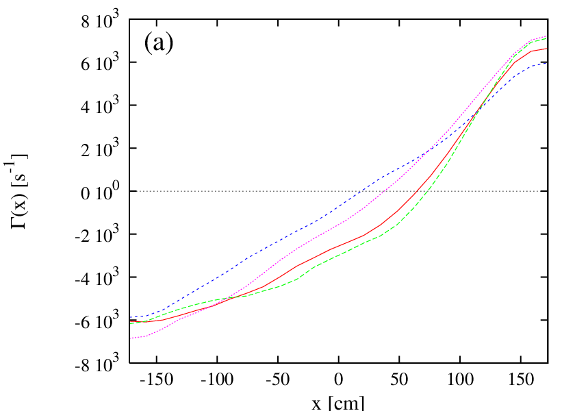
where is the local average velocity and is as usual the particle density. In the following, we focus on the final time, , and we omit as an argument. It turns out that the determination of is very sensitive to the occurrence of large velocities, and due to the symmetry and finiteness of the momentum space used in the solution of the CTRW equations, the local mean found from the solution of the equations is close to zero and cannot be considered meaningful. We thus determine throughout with the use of Monte Carlo simulations, using typically particles to achieve a satisfying numerical precision. Such large numbers of particles are though too expensive in computing time for the critical gradient model, so that we will present only results for the mixed model.
Fig. 15(a) shows as a function of in case of the mixed model, for strong and weak off-axis loading, and for Gaussian and power-law distributed momentum increments, respectively. The location where the flux changes direction (sign) is determined by the change of sign in , which is shown in Fig. 15(b). In all cases shown, there is basically a particle flux from a location in between the density peak and the peak of the off axis source (at ) out-wards to the system boundaries, and both the outflow velocity and the particle flux increase to-wards the boundaries. The particle flux is in all cases shown of the same order of magnitude.
In the classical approach to diffusion, particle transport is traditionally modeled by the equation
| (43) |
together with the assumption that the particle flux is of the form of Fick’s law,
| (44) |
with the diffusivity , and where the pinch velocity is introduced to account for possible anomalous diffusion effects (e.g. Lopez95; the sign convention is such that if then the pinch is in the positive -direction, i.e. motion to the right). To see whether is compatible with the functional form of Eq. (44), we plot in Fig. 15(c) against . For negative values of , the particle flux has the same sign (direction) as , in accordance with Eq. (44), there is though a clear non-uniqueness, where a density gradient can correspond to two, and, in a narrow range, even three different flux values, which is in clear contradiction with Eq. (44). For positive values of , the particle flux can be slightly negative, opposite to the direction of , and, depending on the model, there is a sudden increase at large values of . Last, we note that the particle flux is close to but not zero when the density gradient is zero, which is reminiscent of a small ’off-diagonal’ term, such as a pinch velocity. We thus conclude that the diffusive behaviour is not compatible with the form of Eq. (44), even when assuming non-constant coefficients and , or, in other words, particle transport is not driven by density gradients in the models analyzed, and the characteristics of the particle fluxes we find must be attributed to the strong non-local nature of the diffusion process we study. Similar results concerning non-uniqueness and the particular characteristic shapes of the curves of as a function of have also been reported by vanMil04b for the critical gradient model in position space alone.
Despite the inadequateness of Eq. (44), we can define on the base of Eq. (44) an effective diffusivity,
| (45) |
whereby we neglect a possible pinch velocity. Fig. 15(d) shows the spatial dependence of . In all cases, the diffusivity increases to-wards the edges and it is lowest in the central region, mostly between the center of the box and roughly the peak of the off-axis source at . The singularities appear since the particle fluxes do not vanish there where the density gradient is zero, there is on off-set between the zeros of the fluxes and the zeros of the density gradient. After all, the singularities are the clearest feature in that give a hint that the classical description might not be valid, together with the slightly negative values of in the interval , which indicate that the flux is not in the direction opposite to the density gradient. Thus, the determination of yields a seemingly reasonable picture for the diffusion process, with just minor irregularities, it is though not suited to describe the diffusive processes we study, since Eq. (44) is not an adequate description, as revealed by Fig. 15(c).
Alternatively, the diffusivity can be determined through the more general definition that is based on the scaling of the mean square displacement a particle undergoes in time , as shown in Eq. (1). If we assume that a particle on the average travels from the center of the system to the edge, i.e. a distance , in a time that equals the particle confinement time , then on setting and defining the diffusivity as yields values that are roughly one order of magnitude smaller than in Fig. 15(d). This approach is though again problematic, since the definition of presupposes that diffusion is of classical nature, such that , which would though first have to be confirmed against the more general behaviour of , with characterizing the basic nature of the transport process.

,


IV.2.2 Heat diffusion
The dynamic energy flux is determined as
| (46) |
where we again have assumed and suppress as an argument. Fig. 16(a) shows as a function of for weak and strong off-axis fueling, as yielded by the mixed model for the cases of Gaussian and power-law distributed momentum increments, respectively. The basic shape of the heat fluxes is similar to the ones of the particle fluxes, and the change in direction is again at the locations where changes sign. Notably though, the two cases of power-law distributed momentum increments lead to an almost one order of magnitude higher heat flux than the two cases of Gaussian distributed momentum increments, which must be attributed to the increased energy injection in the acceleration events.
In the classical context, heat diffusion is modeled by
| (47) |
in combination with Fourier’s law for the heat flux,
| (48) |
with the heat diffusivity and a thermal pinch velocity as an additional ’off-diagonal’ term to account for anomalous transport effects (often though, is neglected; e.g. Lopez95). As in the case of the particle flux, it is of interest to see whether the heat fluxes we find are compatible with the form of Eq. (48). In Fig. 16(b), we plot against . Obviously, there are again strong features of non-uniqueness: In case of power-law distributed momentum increments, the non-uniqueness is clearly present for negative and positive values of . In case of Gaussian distributed momentum increments, the non-uniqueness is restricted to positive values of , i.e. negative gradients, which spatially occur in the region from the left edge of the simulation box to the location of the peak of the source at (see Figs. 7(a), 12(a), and 13(a)), and at negative values of , the heat flux is ’uphill’, i.e. opposite to the direction of the negative temperature gradient. In none of the four cases the heat flux is zero when the temperature gradient is zero, which in the frame of Eq. (48) would be interpreted as the presence of an ’off-diagonal term’, e.g. in the form of a pinch velocity. Noteworthy, the non-uniqueness in the cases of Gaussian distributed momentum increments appears despite the fact that the random walk in momentum space is of local nature, and it must be caused by the coupling of momentum space dynamics to the non-local transport in position space. The non-uniqueness, as in case of the particle fluxes, is a result of the non-locality of the process, and it basically makes the transport incompatible with the structure of Eq. (48).
Despite the incompatibility of Eq. (48) with the transport process we study, we define, as in the case of particle diffusion, an effective heat diffusivity
| (49) |
and where we again neglect a possible pinch term. is shown in Fig. 16(c). There occur again singularities, as in case of the particle diffusivity, since the heat flux is not zero there where the temperature gradient is zero. The cases with power-law momentum increments are qualitatively different from the cases with Gaussian momentum increments, basically because the temperature profiles are qualitatively different (see Fig. 13). In the cases with power-law momentum increments, the temperature is peaked near the center, and the temperature gradient has three zeros. The effective diffusivity gives in these cases the following picture: diffusion is reduced in between the temperature peak and the peak of the off-axis injection source, and it increases outside this region to-wards the edges. In the cases of Gaussian momentum increments, heat diffusion is again strongly reduced between the center and the off-axis injection site, and to-wards the edges it is seemingly uphill, in the direction opposite to the negative temperature gradient. Again though it is clear that the picture given by the behaviour of is not representative of the actual diffusion process that is going on, since Eq. (48) is itself not a valid approach.
V Summary and conclusion
We introduced a set of two coupled equations that describe the combined CTRW that includes, besides position space, also momentum space. The equations are of integral form, and they are close to but formally not of the convolution type, so that ways to treat the equations in Fourier Laplace space, e.g. to solve them analytically, to cast them into a different form, or to construct a corresponding fractional diffusion equation, are not obvious.
A way to solve the equations numerically was presented, which is a variant of the pseudospectral method in three dimensional, position-momentum-time space, and it is based on the expansion in terms of Chebyshev polynomials. The method works reliably for the case of linear equations, a method to solve non-linear equations has not yet been developed, so-far. The method could thus be applied only to the mixed model, and not to the critical gradient model, which contains a non-linearity, and for which the presented results were all derived with Monte-Carlo simulations. Monte Carlo simulations were also performed to verify the numerical solution of the combined CTRW equations in case of the mixed model.
In the application to toroidally confined plasmas, we considered an off-axis fueling experiment, with a weak and a strong cold off-axis source, which is known experimentally to give rise to anomalous transport phenomena. Two variants of the combined CTRW have been considered, constructed with the purpose for them to adequately model the specific characteristics of toroidally confined plasmas: (i) the mixed model, where the spatial increments depend on the position of the particles, and (ii) the critical gradient model, in which the position increments depend on the local density gradient.
The main scope in the applications was to reveal what new aspects can be modeled and explained if momentum space is included in a model of non-local, anomalous transport. To explore the role of momentum space dynamics, all applications were done in two versions, one with small, Gaussian distributed momentum increments, which can be interpreted as low-level heating, and one with occasionally large, power-law distributed momentum increments, which corresponds to the case of intense heating. The results can be summarized as follows:
(i) All variants of the mixed and the critical gradient model basically yield peaked density profiles, with a few exceptions of plateau shaped densities. The density profiles exhibit different degrees of stiffness, in the sense of to what degree a model is able to maintain the density peak close to the center in the presence of off-axis sources. The highest stiffness is realized in the mixed model. Generally, intense heating reduces the density profile stiffness.
(ii) The temperature profiles show no stiffness at all with low-level heating, the profiles become though very stiff with intense heating. Intense heating has thus on the temperature profile stiffness the opposite effect it has on the density profile stiffness.
(iii) We find for both models in all variants and independent of the source term an universal distribution of the kinetic energy, namely a power-law with index , also in the cases where the momentum increments follow a Gaussian distribution.
(iv) The particle confinement time is directly proportional to the density, and it is largest for the critical gradient model. Intense heating reduces in all cases the particle confinement time, and therewith the particle density in the system.
(v) The energy confinement time is larger in the critical gradient model than in the mixed model, and, opposite to its effect on the particle confinement, intense heating leads to an increase of the energy confinement time.
(vi) The dynamic particle flux is of simple shape, plotting it though against the density gradient reveals clear features of non-uniqueness, which are a consequence of the non-locality of the transport process, and which make the process incompatible with a classical approach and Fick’s law [Eq. (44)], also when extended with a pinch velocity. The effective particle diffusivity, defined through Fick’s law, gives nonetheless a seemingly reasonable picture.
(vii) The dynamic heat flux is of similar shape as the particle flux, it is though increased by roughly an order of magnitude in the case of intense heating. The heat flux as a function of the temperature gradient also exhibits clear features of non-uniqueness, so that also in this case the classical Fourier’s law [Eq. (48)] is incompatible with the actual heat transport process. This holds true also in the cases where the momentum increments follow a Gaussian distribution and the random walk in momentum space is of classical, quasi-local nature. The effective heat diffusivity determined according to Fourier’s law gives a less reasonable picture than the particle diffusivity, with more singularities and negative values (seeming uphill transport).
We thus conclude that particle and heat diffusivities or pinch velocities determined through a generalized Fick’s and Fourier’s law, respectively, are not adequate tools to characterize a transport process that is of non-local nature in at least the position space, or in position and momentum space.
After all, the inclusion of momentum space truly extends the CTRW formalism, it allows to model new features that belong to momentum space itself, and it substantially modifies and brings forth new aspects of position space dynamics.
Acknowledgements.
The author is grateful to K. Arzner and L. Vlahos for helpful discussions. This work was supported under the Contract of Association ERB 5005 CT 99 0100 between the European Atomic Energy Community and the Hellenic Republic. The sponsors do not bear any responsibility for the contents of this work.Appendix A The pseudospectral method for the solution of integral equations
The pseudospectral method we apply for the solution of the integral equations follows the method in Ref. Mihaila02 for one-dimensional integral equations, which is extended here to the three dimensional case. Detailed properties of Chebyshev polynomials and a description of the pseudospectral method for differential equations can be found e.g. in Ref. Peyret02. The Chebyshev polynomials , which we use as an expansion base, are defined as
| (50) |
for , and where . To use variables in a general interval, , we need to establish a transformation between and . For the cases of position (), and time (), respectively, we choose the simple form
| (51) |
with and . A different choice must be made for the momentum, since the unbounded momentum space should be sufficiently covered with grid points from small to very large momentum values. Evaluating different functional forms, we found best coincidence with Monte-Carlo simulations when introducing a finite momentum interval, and using the transformation
| (52) |
for , and for , and where . The parameters and are adjusted by prescribing the largest () and the smallest () momentum value, which in turn are chosen such that good coincidence with the results from Monte-Carlo simulations is achieved.
The grid points we use are the extrema of in the interval (Gauss-Lobatto grid),
| (53) |
from which the grid-points in the actual position, time, and momentum interval are determined by means of the transformations in Eqs. (51) and (52), respectively,
| (54) |
Before turning to the three dimensional case, we illustrate the Chebyshev expansion in a one-dimensional example: The expansion of a function writes
| (55) |
where is defined as the inverse of the relations in Eqs. (51) (for or ) and (52) (for ), respectively. The double prime on the sum means that the first and the last term of the sum are multiplied by a factor . The expansion coefficients are given as
| (56) |
Following Ref. Mihaila02, it is useful for numerical purposes to reformulate the expansion by inserting the coefficients into Eq. (55), which yields
| (57) |
and in which the expansion coefficients are just the values of the original function at the grid points. In this form, the numerical treatment of the integral equations can be done in direct space, there is no need for transforming to and working in the space of the expansion coefficients.
For the three dimensional case, we first form a tensor product basis, with basis functions
| (58) |
Analogously then to the one dimensional case in Eq. (55), can be expanded as
| (59) |
with the expansion coefficients given by (cf. Eq. (56))
| (60) |
As for Eq. (57) in one dimensions, we insert the expansion coefficients into Eq. (59), so that the expansion is expressed in terms of the values of at the grid points . After rearranging and regrouping the sums, the expansion takes the final form
| (61) | |||||
Turning now to the integral equation for , Eq. (19), we insert the expansion of Eq. (61) for under the integral in Eq. (19), which yields
| (62) | |||||
In the same way, Eq. (25) for is treated, we insert Eq. (61) for under the integral, which leads to
| (63) | |||||
The next step consists in collocating the equations, i.e. we consider the equations only at the grid points and replace the free variables by their values at the grid-points, with the free indices running over the same range as the indices . In this way, Eq. (62) for takes the form
| (64) | |||||
In the last step, we remove the double primes on the sums, introducing the explicit factors
| (65) |
and we rearrange the sums and integrals in Eq. (64) such that the structure of their mutual dependencies becomes more obvious,
| (66) | |||||
If the distributions of increments and do not contain any information on and , as in the case of the mixed model, then the integrals are over given functions and can be done with any appropriate numerical method. Eq. (66) is then a linear equation for the values of at the grid points, and it can be solved with any numerical method for linear systems of equations.
The propagator is determined by collocating Eq. (63) at the grid points [, in the same way as for in Eq. (64)], which, after rearranging the sums and integrals, yields
| (67) | |||||
Again, if the pdf of increments are independent of , then the integrals are over given functions, and Eq. (67) can be interpreted as a simple matrix multiplication that yields the values of at the grid points from the value of at the grid-points.
References
- (1) Bak, P., Tang, C., Wiesenfeld, K., Phys. Rev. Lett. 59, 381 (1987)
- (2) Baker, D.R., Greenfield, C.M., Burnell, K.H., et al, Phys. of Plasmas 8, 4128 (2001).
- (3) Balescu, R., Phys. Rev. E 51, 4807 (1995)
- (4) Hoang, G.T., Bourdelle, C., Garbet, X., et al., Phys. Rev. Lett. 87, 125001-1 (2001)
- (5) Isliker, H., Vlahos, L., Phys. Rev. E 67,026413 (2003).
- (6) Garbet, X., Mantica, P., Angioni, C., et al., Plasma Phys. Control. Fusion 46, B557 (2004).
- (7) Garbet, X., Mantica, P., Ryter, F., et al., Plasma Phys. Control. Fusion 46, 1351 (2004).
- (8) Imbeau, F., Ryter, F., Garbet, X., Plasma Phys. Control. Fusion 43, 1503 (2001).
- (9) Jackson, J.D., Classical Electrodynamics, John Wiley & Sons, New York, 1962
- (10) Lemoine, N., Gresillon, D.M., Phys. of Plasmas 12, 092301 (2005).
- (11) Lopes Cardoso, N.J., Plasma Phys. Control. Fusion 37, 799 (1995).
- (12) Luce, T.C., Petty, C.C., der Haas, J.C.M., Phys. Rev. Lett. 68, 52, (1992)
- (13) Mihaila, B., Mihaila, I., J. Phys. A 35, 731 (2002),
- (14) van Milligen, B. Ph., Sánchez, R., Carreras, B.A., Phys. of Plasmas 11, 2272 (2004)
- (15) van Milligen, B. Ph., Carreras, B.A., Sánchez, R., Physics of Plasmas 11, 3787 (2004).
- (16) Metzler, R., Klafter, J., Physics Reports 339, 1 (2000).
- (17) E.W. Montroll, G.H. Weiss, J. Math. Phys. 6, 167 (1965).
- (18) Petty, C.C., Luce, T.C., Nuclear Fusion 34, 121 (1994)
- (19) Peyret, R., Spectral Methods for Incompressible Viscous Flow (Applied mathematical sciences 148), Berlin (Springer-Verlag, Berlin), 2002.
- (20) Ryter, F., Angioni, C., Beurskens, M., et al., Plasma Phys. and Control. Fusion 43, A323 (2001).
- (21) Ryter, F., Tardoni, G., De Luca, F., et al. Nuclear Fusion 43, 1396 (2003).
- (22) Shlesinger, M.F., West, B., Klafter, J., Phys. Rev. Lett. 58, 1100 (1987).
- (23) Vlahos, L., Isliker, H., Lepreti, F., Astrophys. Journ. 608, 540 (2004).
- (24) Zumofen, G., Klafter, J., Phys. Rev. E 47, 851 (1993).