跳到论文正文
W Papers独立论文阅读器 arXiv:0710.4987 论文正文 计算阅读时间 · 0%
引用这篇论文根据当前论文元数据生成,正式投稿前建议核对。


License: Assumed arXiv.org perpetual non-exclusive license
arXiv:0710.4987v1 [cs.IT] 26 Oct 2007

Universal source coding over generalized complementary delivery networks

Akisato Kimura       Tomohiko Uyematsu       Shigeaki Kuzuoka          Shun Watanabe    Thanks: A. Kimura is with NTT Communication Science Laboratories, NTT Corporation, 3-1 Morinosato Wakamiya, Atsugi-shi, Kanagawa, 243-0198 Japan. E-mail: research@akisato.org Thanks: T. Uyematsu and S. Watanabe are with Department of Communications and Integrated Systems, Tokyo Institute of Technology, 2-12-1 Ookayama, Meguro-ku, Tokyo, 152-8552 Japan. E-mail: uyematsu@ieee.org, shun-wata@it.ss.titech.ac.jp Thanks: S. Kuzuoka is with Department of Computer and Communication Sciences, Wakayama University, 930 Sakaedani, Wakayama, Wakayama 640-8510 Japan. E-mail: kuzuoka@sys.wakayama-u.ac.jp Thanks: Manuscript received October 26, 2007.
Abstract

This paper deals with a universal coding problem for a certain kind of multiterminal source coding network called a generalized complementary delivery network. In this network, messages from multiple correlated sources are jointly encoded, and each decoder has access to some of the messages to enable it to reproduce the other messages. Both fixed-to-fixed length and fixed-to-variable length lossless coding schemes are considered. Explicit constructions of universal codes and the bounds of the error probabilities are clarified by using methods of types and graph-theoretical analysis.

Index Terms: 
multiterminal source coding, network source coding, correlated sources, universal coding, lossless coding, complementary delivery, vertex coloring, methods of types.

I Introduction

A coding problem for correlated information sources was first described and investigated by Slepian and Wolf [1], and later, various coding problems derived from that work were considered (e.g. Wyner [2], Ko¨\ddot{\mbox{o}}rner and Marton [3], Sgarro [4]). Meanwhile, the problem of universal coding for these systems was first investigated by Csisza´\acute{\mbox{a}}r and Ko¨\ddot{\mbox{o}}rner [5]. Universal coding problems are not only interesting in their own right but are also very important in terms of practical applications. Subsequent work has mainly focused on the Slepian-Wolf network [6, 7, 8] since it appears to be difficult to construct universal codes for most of the other networks. For example, Muramatsu [9] showed that no fixed-to-variable length (FV) universal code can attain the optimal coding rate for the Wyner-Ziv coding problem[10].

Refer to caption
Fig. 1: Data collection: Stations are physically separated from each other. Each station collects its own target data, and transmits them to a satellite.
Refer to caption
Fig. 2: Data distribution: The satellite broadcasts the collected data back to the stations for sharing. Each station has already gathered its own target data, and thus wants to reproduce the other data by using its own target data as side information.

Our main contributions in this paper include showing explicit constructions of universal codes for other multiterminal source coding networks. Figs. 2 and 2 illustrate the scenario we are considering: Several stations are separately deployed in a field. Every station collects its own target data from sensors or terminals, and wants to share all the target data with the other stations. To accomplish this task, each station transmits the collected data to a satellite, and the satellite broadcasts all the received data back to the stations. Each station utilizes its own target data as side information to reproduce all the other data. Willems et al. [11, 12] investigated a special case of the above scenario in which three stations were deployed and each station had access to one of three target messages, and they determined the minimum achievable rates for uplink (from each station to the satellite) and downlink (from the satellite to all the stations) transmissions. Their main result implies that the uplink transmission is equivalent to the traditional Slepian-Wolf coding system [1], and thus we should concentrate on the downlink part. Henceforth we denote the networks characterized by the downlink transmission shown in Fig. 2 as generalized complementary delivery networks (Fig. 3), and we denote the generalized complementary delivery network with two stations and two target messages as the (original) complementary delivery network. This notation is based on the network structure where each station (decoder) complements the target messages from the codeword delivered by the satellite (encoder).

Refer to caption
Fig. 3: Generalized complementary delivery network

The complementary delivery network can be regarded as a special example of the butterfly network [13, 14] (Fig.4), which is one of a very well known network structure that represents the benefits of network coding. If we assume that all the edges in Fig. 4 except that between nodes 3 and 4 have sufficiently large capacities, the problem is to find the minimum capacities of the edge between the nodes 3 and 4 satisfying that allows two messages emitted from the source (node 0) to be delivered to sinks 1 (node 5) and 2 (node 6). This situation is equivalent to the complementary delivery network in which the messages emitted from the source node are correlated with each other. Several coding problems for correlated sources over a network have recently been investigated. At first only one receiver was considered (e.g. [15, 16]) , and later networks incorporating multiple receivers were studied (e.g. [17, 18, 19, 20]). In particular, Ho et al. [18] and Kuzuoka et al. [20] applied the linear Slepian-Wolf codes to random linear network coding over general 2-source multi-cast networks and universal source coding for the complementary delivery network, respectively. However, explicit code constructions over networks with multiple sources and multiple destinations still remain open.

Refer to caption
Fig. 4: Butterfly network

This paper proposes a universal coding scheme for generalized complementary delivery networks that involve multiple sources and multiple destinations. First, an explicit construction of fixed-to-fixed length (FF) universal codes based on a graph-theoretical analysis is presented. This construction utilizes a codebook expressed as a certain kind of undirected graphs. Encoding can be regarded as the vertex coloring of the graphs. The bounds of error probabilities and probabilities of correct decoding can be evaluated by methods of types. The proposed coding scheme can always attain the optimal error exponent (the exponent of error probabilities), and can attain the optimal exponent of correct decoding in some cases. This FF coding scheme can be applied to fixed-to-variable length (FV) universal codes. Overflow and underflow probabilities are evaluated in almost the same way as the error probabilities and the probabilities of correct decoding, respectively.

This paper is organized as follows: Notations and definitions are provided in Section II. A generic formulation of the generalized complementary delivery coding system is introduced in Section III. A coding scheme for FF universal codes is proposed in Section IV. Several coding theorems for FF universal codes are clarified in Section V. Lastly, FV universal coding is discussed in Section VI.

II Preliminaries

II-A Basic definitions

Let ℬ\mathcal{B} be a binary set, ℬ∗\mathcal{B}^{*} be the set of all finite sequences in the set ℬ\mathcal{B} and ℐM={1,2,⋯,M}\mathcal{I}_{M}=\{1,2,\cdots,M\} for an integer MM. In what follows, random variables are denoted by capital letters such as XX, and their sample values (resp. alphabets) by the corresponding small letters (resp. calligraphic letters) such as xx (resp. 𝒳\mathcal{X}), except as otherwise noted. The cardinality of a finite set 𝒳\mathcal{X} is written as |𝒳||\mathcal{X}|, and the nn-th Cartesian product of 𝒳\mathcal{X} by 𝒳n\mathcal{X}^{n}. A member of 𝒳n\mathcal{X}^{n} is written as

xn=(x1,x2,⋯,xn),x^{n}=(x_{1},x_{2},\cdots,x_{n}),

and substrings of xnx^{n} are written as

xij=(xi,xi+1,⋯,xj)i≤j.x_{i}^{j}=(x_{i},x_{i+1},\cdots,x_{j})\quad i\leq j.

When the dimension is clear from the context, vectors will be denoted by boldface letters, i.e., 𝒙∈𝒳n\boldsymbol{x}\in\mathcal{X}^{n}.

The probability distribution for a random variable XX is denoted by PXP_{X}. Similarly, the probability distribution for random variables (X,Y)(X,Y) is denoted by PX​YP_{XY}, and the conditional distribution of XX given YY is written as PX|YP_{X|Y}. The set of all probability distributions on 𝒳\mathcal{X} is written as 𝒫⁡(𝒳)\mathcal{P}(\mathcal{X}), and the set of all conditional distributions on 𝒳\mathcal{X} given a distribution PY∈𝒫⁡(𝒴)P_{Y}\in\mathcal{P}(\mathcal{Y}) is written as 𝒫⁡(𝒳|PY)\mathcal{P}(\mathcal{X}|P_{Y}), which means that each member PX|YP_{X|Y} of 𝒫⁡(𝒳|PY)\mathcal{P}(\mathcal{X}|P_{Y}) is characterized by PX​Y∈𝒫⁡(𝒳×𝒴)P_{XY}\in\mathcal{P}(\mathcal{X}\times\mathcal{Y}) as PX​Y=PX|Y​PYP_{XY}=P_{X|Y}P_{Y}. A discrete memoryless source (DMS) is an infinite sequence of independent copies of a random variable XX. The alphabet of a DMS is assumed to be a finite set except as otherwise noted. For simplicity, we denote a source (𝒳,PX)(\mathcal{X},P_{X}) by referring to its generic distribution PXP_{X} or random variable XX. A set

𝑿=(X(1),X(2),⋯,X(Ns))\boldsymbol{X}=(X^{(1)},X^{(2)},\cdots,X^{(N_{s})})

of NsN_{s} random variables is also called a DMS, where each random variable X(i)X^{(i)} takes a value in a finite set 𝒳(i)\mathcal{X}^{(i)} (i∈ℐNs)(i\in\mathcal{I}_{N_{s}}). For a set 𝒮⊆ℐNs\mathcal{S}\subseteq\mathcal{I}_{N_{s}}, the corresponding subset of sources is written as

𝑿(𝒮)\displaystyle\boldsymbol{X}^{(\mathcal{S})} =def.\displaystyle{\displaystyle\mathop{=}^{\mbox{\rm def.}}} {X(i)|i∈𝒮},\displaystyle\{X^{(i)}|i\in\mathcal{S}\},

and the corresponding subset of its sample sequences (resp. alphabets) 𝒮\mathcal{S} is denoted by

𝒳(𝒮)\displaystyle\mathcal{X}^{(\mathcal{S})} =def.\displaystyle{\displaystyle\mathop{=}^{\mbox{\rm def.}}} ∏i∈𝒮𝒳(i),\displaystyle\prod_{i\in\mathcal{S}}\mathcal{X}^{(i)},
𝒙(𝒮)\displaystyle\boldsymbol{x}^{(\mathcal{S})} =def.\displaystyle{\displaystyle\mathop{=}^{\mbox{\rm def.}}} {𝒙(i)∈𝒳(i)|i∈𝒮}.\displaystyle\{\boldsymbol{x}^{(i)}\in\mathcal{X}^{(i)}|i\in\mathcal{S}\}.

For a set 𝒮⊆ℐNs\mathcal{S}\subseteq\mathcal{I}_{N_{s}}, the nn-th Cartesian product of 𝒳(𝒮)\mathcal{X}^{(\mathcal{S})}, its member and the corresponding random variable are written as 𝒳(𝒮)​n\mathcal{X}^{(\mathcal{S})n}, 𝒙(𝒮)​n\boldsymbol{x}^{(\mathcal{S})n} and 𝑿(𝒮)​n\boldsymbol{X}^{(\mathcal{S})n}, respectively. With 𝒮=ℐNs\mathcal{S}=\mathcal{I}_{N_{s}}, we denote 𝑿(𝒮)​n=𝑿n\boldsymbol{X}^{(\mathcal{S})n}=\boldsymbol{X}^{n}. For a set 𝒮⊆ℐNs\mathcal{S}\subseteq\mathcal{I}_{N_{s}}, its complement is denoted as 𝒮c=ℐNs−𝒮\mathcal{S}^{c}=\mathcal{I}_{N_{s}}-\mathcal{S}.

For a DMS 𝑿\boldsymbol{X} and finite sets 𝒮1,𝒮2⊆ℐNs\mathcal{S}_{1},\mathcal{S}_{2}\subseteq\mathcal{I}_{N_{s}} that satisfy 𝒮1∩𝒮2=∅\mathcal{S}_{1}\cap\mathcal{S}_{2}=\emptyset, the joint entropy of 𝑿(𝒮1)\boldsymbol{X}^{(\mathcal{S}_{1})} and the conditional entropy of 𝑿(𝒮2)\boldsymbol{X}^{(\mathcal{S}_{2})} given 𝑿(𝒮1)\boldsymbol{X}^{(\mathcal{S}_{1})} are written as H⁡(𝑿(𝒮1))H(\boldsymbol{X}^{(\mathcal{S}_{1})}) and H⁡(𝑿(𝒮2)|𝑿(𝒮1))H(\boldsymbol{X}^{(\mathcal{S}_{2})}|\boldsymbol{X}^{(\mathcal{S}_{1})}), respectively (cf. [21]). For a generic distribution P∈𝒫⁡(𝒳(𝒮1))P\in\mathcal{P}(\mathcal{X}^{(\mathcal{S}_{1})}) and a conditional distribution W∈𝒫⁡(𝒳(𝒮2)|P)W\in\mathcal{P}(\mathcal{X}^{(\mathcal{S}_{2})}|P), H⁡(P)H(P) and H⁡(W|P)H(W|P) also represent the joint entropy of 𝑿(𝒮1)\boldsymbol{X}^{(\mathcal{S}_{1})} and the conditional entropy of 𝑿(𝒮2)\boldsymbol{X}^{(\mathcal{S}_{2})} given 𝑿(𝒮1)\boldsymbol{X}^{(\mathcal{S}_{1})}, where P=P𝑿(𝒮1)P=P_{\boldsymbol{X}^{(\mathcal{S}_{1})}} and W=P𝑿(𝒮2)|𝑿(𝒮1)W=P_{\boldsymbol{X}^{(\mathcal{S}_{2})}|\boldsymbol{X}^{(\mathcal{S}_{1})}}. The Kullback-Leibler divergence, or simply the divergence, between two distributions PP and QQ is written as D(P∥Q)D(P\|Q).

In the following, all bases of exponentials and logarithms are set at 2.

II-B Types of sequences

Let us define the type of a sequence 𝒙∈𝒳n\boldsymbol{x}\in\mathcal{X}^{n} as the empirical distribution Q𝒙∈𝒫⁡(𝒳)Q_{\boldsymbol{x}}\in\mathcal{P}(\mathcal{X}) of the sequence 𝒙\boldsymbol{x}, i.e.

Q𝒙​(a)\displaystyle Q_{\boldsymbol{x}}(a) =def.\displaystyle{\displaystyle\mathop{=}^{\mbox{\rm def.}}} 1n​N​(a|𝒙)∀a∈𝒳,\displaystyle\frac{1}{n}N(a|\boldsymbol{x})\quad\forall a\in\mathcal{X},

where N⁡(a|𝒙)N(a|\boldsymbol{x}) represents the number of occurrences of the letter aa in the sequence 𝒙\boldsymbol{x}. Similarly, the joint type Q𝒙(𝒮)∈𝒫⁡(𝒳𝒮)Q_{\boldsymbol{x}^{(\mathcal{S})}}\in\mathcal{P}(\mathcal{X}^{\mathcal{S}}) for a given set 𝒮⊆ℐNs\mathcal{S}\subseteq\mathcal{I}_{N_{s}} is defined by

Q𝒙(𝒮)​(ai1,ai2,⋯,ai|𝒮|)\displaystyle Q_{\boldsymbol{x}^{(\mathcal{S})}}(a_{i_{1}},a_{i_{2}},\cdots,a_{i_{|\mathcal{S}|}})
=def.\displaystyle{\displaystyle\mathop{=}^{\mbox{\rm def.}}} 1n​N​(ai1,ai2,⋯,ai|𝒮||𝒙(𝒮))\displaystyle\frac{1}{n}N(a_{i_{1}},a_{i_{2}},\cdots,a_{i_{|\mathcal{S}|}}|\boldsymbol{x}^{(\mathcal{S})})
∀(ai1,ai2,⋯,ai|𝒮|)∈𝒳(𝒮).\displaystyle\forall(a_{i_{1}},a_{i_{2}},\cdots,a_{i_{|\mathcal{S}|}})\in\mathcal{X}^{(\mathcal{S})}.

Let 𝒫n​(𝒳)\mathcal{P}_{n}(\mathcal{X}) be the set of types of sequences in 𝒳n\mathcal{X}^{n}. Similarly, for every type Q∈𝒫n​(𝒳)Q\in\mathcal{P}_{n}(\mathcal{X}), let 𝒱n​(𝒴|Q)\mathcal{V}_{n}(\mathcal{Y}|Q) be the set of all stochastic matrices V:𝒳→𝒴V:\mathcal{X}\to\mathcal{Y} such that for some pairs (𝒙,𝒚)∈𝒳n×𝒴n(\boldsymbol{x},\boldsymbol{y})\in\mathcal{X}^{n}\times\mathcal{Y}^{n} of sequences we have

Q𝒙,𝒚​(𝒙,𝒚)=Q⁡(𝒙)​V​(𝒚|𝒙)=∏i=1nQ⁡(xi)​V​(yi|xi).Q_{\boldsymbol{x},\boldsymbol{y}}(\boldsymbol{x},\boldsymbol{y})=Q(\boldsymbol{x})V(\boldsymbol{y}|\boldsymbol{x})=\prod_{i=1}^{n}Q(x_{i})V(y_{i}|x_{i}).

For every type Q∈𝒫n​(𝒳)Q\in\mathcal{P}_{n}(\mathcal{X}) we denote

TQn​=def.{𝒙∈𝒳n|Q𝒙=Q}.T_{Q}^{n}~{\displaystyle\mathop{=}^{\mbox{\rm def.}}}~\{\boldsymbol{x}\in\mathcal{X}^{n}|Q_{\boldsymbol{x}}=Q\}.

Similarly, for every sequence 𝒙∈TQn\boldsymbol{x}\in T_{Q}^{n} and stochastic matrix V∈𝒱n​(𝒴|Q)V\in\mathcal{V}_{n}(\mathcal{Y}|Q), we define a V-shell as

TVn(𝒙)=def.\displaystyle T_{V}^{n}(\boldsymbol{x}){\displaystyle\mathop{=}^{\mbox{\rm def.}}}
{𝒚∈𝒴n|Q(x)V(y|x)=Q𝒙,𝒚(x,y),∀(x,y)∈𝒳×𝒴}.\displaystyle\{\boldsymbol{y}\in\mathcal{Y}^{n}|Q(x)V(y|x)=Q_{\boldsymbol{x},\boldsymbol{y}}(x,y),~\forall(x,y)\in\mathcal{X}\times\mathcal{Y}\}.

Here, let us introduce several important properties of types.

Lemma 1

(Type counting lemma [21, Lemma 2.2])

|𝒫n​(𝒳)|≤(n+1)|𝒳|.|\mathcal{P}_{n}(\mathcal{X})|\leq(n+1)^{|\mathcal{X}|}.
Lemma 2

(Sizes of V-shells [21, Lemma 2.5])
For every type Q∈𝒫n​(𝒳)Q\in\mathcal{P}_{n}(\mathcal{X}), sequence 𝐱∈TQn\boldsymbol{x}\in T_{Q}^{n} and stochastic matrix V:𝒳→𝒴V:\mathcal{X}\to\mathcal{Y} such that TVn​(𝐱)≠∅T_{V}^{n}(\boldsymbol{x})\neq\emptyset, we have

|TVn​(𝒙)|\displaystyle|T_{V}^{n}(\boldsymbol{x})| ≥\displaystyle\geq (n+1)−|𝒳|​|𝒴|​exp⁡{n​H​(V|Q)},\displaystyle(n+1)^{-|\mathcal{X}||\mathcal{Y}|}\exp\{nH(V|Q)\},
|TVn​(𝒙)|\displaystyle|T_{V}^{n}(\boldsymbol{x})| ≤\displaystyle\leq exp⁡{n​H​(V|Q)}.\displaystyle\exp\{nH(V|Q)\}.
Lemma 3

(Probabilities of types [21, Lemma 2.6])
For every type Q∈𝒫n​(𝒳)Q\in\mathcal{P}_{n}(\mathcal{X}) and every distribution PX∈𝒫⁡(𝒳)P_{X}\in\mathcal{P}(\mathcal{X}), we have

PX​(𝒙)\displaystyle P_{X}(\boldsymbol{x}) =\displaystyle= exp{−n(D(Q∥PX)+H(Q))}∀𝒙∈TQ,\displaystyle\exp\{-n(D(Q\|P_{X})+H(Q))\}\quad\forall\boldsymbol{x}\in T_{Q},
PX​(TQ)\displaystyle P_{X}(T_{Q}) ≥\displaystyle\geq (n+1)−|𝒳|exp{−nD(Q∥PX)},\displaystyle(n+1)^{-|\mathcal{X}|}\exp\{-nD(Q\|P_{X})\},
PX​(TQ)\displaystyle P_{X}(T_{Q}) ≤\displaystyle\leq exp{−nD(Q∥PX)}.\displaystyle\exp\{-nD(Q\|P_{X})\}.

II-C Graph coloring

Let us introduce several notations and lemmas related to graph coloring. A (undirected) graph is denoted as G=(VG,EG)G=(V_{G},E_{G}), where VGV_{G} is a set of vertices and EGE_{G} is a set of edges. The degree Δ⁡(v)\Delta(v) of a vertex v∈VGv\in V_{G} is the number of other vertices connected by edges, and the degree Δ⁡(G)\Delta(G) of a graph is the maximum number of degrees of vertices in the graph GG. A graph where an edge connects every pair of vertices is called a complete graph. A complete subgraph is called a clique, and the largest degree of cliques in a graph GG is called the clique number ω⁡(G)\omega(G) of the graph GG. The vertex coloring, or simply coloring of a graph GG is where no two adjacent vertices are assigned the same symbol. The number of symbols necessary for the vertex coloring of a graph is called the chromatic number χ⁡(G)\chi(G). Similarly, the edge coloring of a graph GG is where no two adjacent edges are assigned the same symbol, and the number of symbols necessary for edge coloring is called the edge chromatic number χ′​(G)\chi^{\prime}(G).

The following lemmas are well known as bounds of the chromatic number and the edge chromatic number.

Lemma 4

(Brooks [22, 23])

ω⁡(G)≤χ⁡(G)≤Δ⁡(G)\displaystyle\omega(G)\leq\chi(G)\leq\Delta(G)

unless GG is a complete graph or an odd cycle (a cycle graph that contains an odd number of vertices).

Lemma 5

(Vizing [24, 23])

Δ⁡(G)≤χ′​(G)≤Δ⁡(G)+1.\displaystyle\Delta(G)\leq\chi^{\prime}(G)\leq\Delta(G)+1.
Lemma 6

(Ko¨\ddot{\mbox{o}}nig [25, 23])
If a graph GG is bipartite, then

χ′​(G)=Δ​(G).\displaystyle\chi^{\prime}(G)=\Delta(G).

III Problem formulation

This section formulates the coding problem investigated in this paper, and shows the fundamental bound of the coding rate.

First, we describe a generalized complementary delivery network. Fig. 3 represents the network formulated below. This network is composed of NsN_{s} sources 𝑿=𝑿(ℐNs)\boldsymbol{X}=\boldsymbol{X}^{(\mathcal{I}_{N_{s}})}, one encoder φn\varphi_{n} and NdN_{d} decoders φ^n(1)\widehat{\varphi}_{n}^{(1)} ⋯φ^n(Nd)\cdots\widehat{\varphi}_{n}^{(N_{d})}. Each decoder φ^n(j)\widehat{\varphi}_{n}^{(j)} has access to side information 𝑿(𝒮jc)\boldsymbol{X}^{(\mathcal{S}_{j}^{c})} (𝒮j⊂ℐNs)(\mathcal{S}_{j}\subset\mathcal{I}_{N_{s}}) to enable it to reproduce the information 𝑿(𝒮j)\boldsymbol{X}^{(\mathcal{S}_{j})}. Since the indices 𝓢={𝒮j}j=1Nd\boldsymbol{\mathcal{S}}=\{\mathcal{S}_{j}\}_{j=1}^{N_{d}} of side information determine the network, henceforth we denote the network by 𝓢\boldsymbol{\mathcal{S}}. Without loss of generality, we assume 𝒮j1≠𝒮j2\mathcal{S}_{j_{1}}\neq\mathcal{S}_{j_{2}} ∀j1,j2∈ℐNd\forall j_{1},j_{2}\in\mathcal{I}_{N_{d}}.

Based on the above definition of the network, we formulate the coding problem for the network.

Definition 1

(Fixed-to-fixed generalized complementary delivery (FF-GCD) code)
A sequence

{(φn,φ^n(1),⋯,φ^n(Nd))}n=1∞\{(\varphi_{n},\widehat{\varphi}_{n}^{(1)},\cdots,\widehat{\varphi}_{n}^{(N_{d})})\}_{n=1}^{\infty}

of codes

(φn,φ^n(1),⋯,φ^n(Nd))(\varphi_{n},\widehat{\varphi}_{n}^{(1)},\cdots,\widehat{\varphi}_{n}^{(N_{d})})

is an FF-GCD code for the network 𝓢={𝒮j}j=1Nd\boldsymbol{\mathcal{S}}=\{\mathcal{S}_{j}\}_{j=1}^{N_{d}} if

φn\displaystyle\varphi_{n} :\displaystyle: 𝒳(ℐNs)​n→ℐMn\displaystyle\mathcal{X}^{(\mathcal{I}_{N_{s}})n}\rightarrow\mathcal{I}_{M_{n}}
φ^n(j)\displaystyle\widehat{\varphi}_{n}^{(j)} :\displaystyle: ℐMn×𝒳(𝒮jc)​n→𝒳(𝒮j)​n∀j∈ℐNd.\displaystyle\mathcal{I}_{M_{n}}\times\mathcal{X}^{(\mathcal{S}_{j}^{c})n}\rightarrow\mathcal{X}^{(\mathcal{S}_{j})n}\quad\forall j\in\mathcal{I}_{N_{d}}.
Definition 2

(FF-GCD achievable rate)
RR is an FF-GCD achievable rate of the source 𝐗\boldsymbol{X} for the network 𝓢\boldsymbol{\mathcal{S}} if and only if there exists an FF-GCD code

{(φn,φ^n(1),⋯,φ^n(Nd))}n=1∞\{(\varphi_{n},\widehat{\varphi}_{n}^{(1)},\cdots,\widehat{\varphi}_{n}^{(N_{d})})\}_{n=1}^{\infty}

for the network 𝓢\boldsymbol{\mathcal{S}} that satisfies

lim supn→∞1n​log⁡Mn\displaystyle\limsup_{n\to\infty}\frac{1}{n}\log M_{n} ≤\displaystyle\leq R,\displaystyle R,
limn→∞en(j)\displaystyle\lim_{n\to\infty}e_{n}^{(j)} =\displaystyle= 0∀j∈ℐNd.\displaystyle 0\quad\forall j\in\mathcal{I}_{N_{d}}.

where

en(j)\displaystyle e_{n}^{(j)} =\displaystyle= Pr{𝑿(𝒮j)​n≠𝑿^(𝒮j)​n}∀j∈ℐNd,\displaystyle\Pr\left\{\boldsymbol{X}^{(\mathcal{S}_{j})n}\neq\widehat{\boldsymbol{X}}^{(\mathcal{S}_{j})n}\right\}\quad\forall j\in\mathcal{I}_{N_{d}},
𝑿^(𝒮j)​n\displaystyle\widehat{\boldsymbol{X}}^{(\mathcal{S}_{j})n} =def.\displaystyle{\displaystyle\mathop{=}^{\mbox{\rm def.}}} φ^n(j)​(φn​(𝑿n),𝑿(𝒮jc)​n).\displaystyle\widehat{\varphi}_{n}^{(j)}(\varphi_{n}(\boldsymbol{X}^{n}),\boldsymbol{X}^{(\mathcal{S}_{j}^{c})n}).
Definition 3

(Inf FF-GCD achievable rate)

Rf​(𝑿|𝓢)\displaystyle R_{f}(\boldsymbol{X}|\boldsymbol{\mathcal{S}})
=\displaystyle= inf{R|R​ is an FF-GCD achievable rate of ​𝑿​ for ​𝓢}.\displaystyle\inf\{R|R\mbox{ is an FF-GCD achievable rate of }\boldsymbol{X}\mbox{ for }\boldsymbol{\mathcal{S}}\}.
Refer to caption
Fig. 5: Network investigated by Willems et al.

Willems et al. [11, 12] clarified the minimum achievable rate Rf​(𝑿|𝓢)R_{f}(\boldsymbol{X}|\boldsymbol{\mathcal{S}}) for a special case, where Ns=Nd=3N_{s}=N_{d}=3, (X1,X2,X3)=(X,Y,Z)(X_{1},X_{2},X_{3})=(X,Y,Z), 𝒮1={1,2}\mathcal{S}_{1}=\{1,2\}, 𝒮2={1,3}\mathcal{S}_{2}=\{1,3\} and 𝒮3={2,3}\mathcal{S}_{3}=\{2,3\} (Fig. 5).

Theorem 1

(Coding theorem of FF-GCD codes for three users [12])
If Ns=Nd=3N_{s}=N_{d}=3, (X1,X2,X3)=(X,Y,Z)(X_{1},X_{2},X_{3})=(X,Y,Z), 𝒮1={1,2}\mathcal{S}_{1}=\{1,2\}, 𝒮2={1,3}\mathcal{S}_{2}=\{1,3\} and 𝒮3={2,3}\mathcal{S}_{3}=\{2,3\}, then

Rf​(X,Y,Z|𝓢)\displaystyle R_{f}(X,Y,Z|\boldsymbol{\mathcal{S}})
=\displaystyle= max⁡{H⁡(X,Y|Z),H⁡(Y,Z|X),H⁡(X,Z|Y)}\displaystyle\max\{H(X,Y|Z),H(Y,Z|X),H(X,Z|Y)\}

It is easy to extend Theorem 1 to the following coding theorem for general cases:

Theorem 2

(Coding theorem of FF-GCD codes for general cases)

Rf​(𝑿|𝓢)\displaystyle R_{f}(\boldsymbol{X}|\boldsymbol{\mathcal{S}}) =\displaystyle= maxj∈ℐNdH(𝑿(𝒮j)|𝑿(𝒮jc))\displaystyle\max_{j\in\mathcal{I}_{N_{d}}}H\left(\boldsymbol{X}^{(\mathcal{S}_{j})}\left|\boldsymbol{X}^{(\mathcal{S}_{j}^{c})}\right.\right)
Remark 1

The generalized complementary delivery network is included in the framework considered by Csisza´\acute{\mbox{a}}r and Ko¨\ddot{\mbox{o}}rner [5]. Therefore, Theorem 2 can be obtained as a corollary of their results.

IV Code construction

This section shows an explicit construction of universal codes for the generalized complementary delivery network. The proposed universal coding scheme is described as follows:

Refer to caption
Refer to caption
Refer to caption
Refer to caption
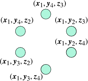
Fig. 6: (Upper left) Intuitive example of coding graph. Each node corresponds to a sequence set (𝒙i,𝒚j,𝒛k)∈TQX​Y​Zn(\boldsymbol{x}_{i},\boldsymbol{y}_{j},\boldsymbol{z}_{k})\in T_{Q_{XYZ}}^{n}.
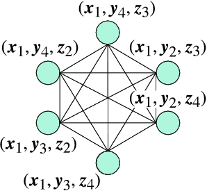
Fig. 7: (Upper right) For a given 𝒙1\boldsymbol{x}_{1}, an edge is placed between every pair of vertices whose subsequences satisfy (𝒚j,𝒛k)∈TV3n​(𝒙1)(\boldsymbol{y}_{j},\boldsymbol{z}_{k})\in T_{V_{3}}^{n}(\boldsymbol{x}_{1}), which means that for a given 𝒙1\boldsymbol{x}_{1} we must distinguish each (𝒚j,𝒛k)(\boldsymbol{y}_{j},\boldsymbol{z}_{k}) such that (𝒙1,𝒚j,𝒛k)∈TQX​Y​Zn(\boldsymbol{x}_{1},\boldsymbol{y}_{j},\boldsymbol{z}_{k})\in T_{Q_{XYZ}}^{n}.
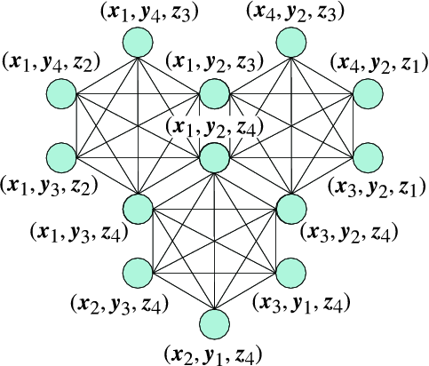
Fig. 8: (Lower left) In a similar manner, for a given 𝒚2\boldsymbol{y}_{2} (resp. 𝒛4\boldsymbol{z}_{4}) an edge is deployed between every pair of vertices whose subsequences satisfy (𝒙i,𝒛k)∈TV2n​(𝒚2)(\boldsymbol{x}_{i},\boldsymbol{z}_{k})\in T_{V_{2}}^{n}(\boldsymbol{y}_{2}) (resp. (𝒙i,𝒚j)∈TV1n​(𝒛4)(\boldsymbol{x}_{i},\boldsymbol{y}_{j})\in T_{V_{1}}^{n}(\boldsymbol{z}_{4})).
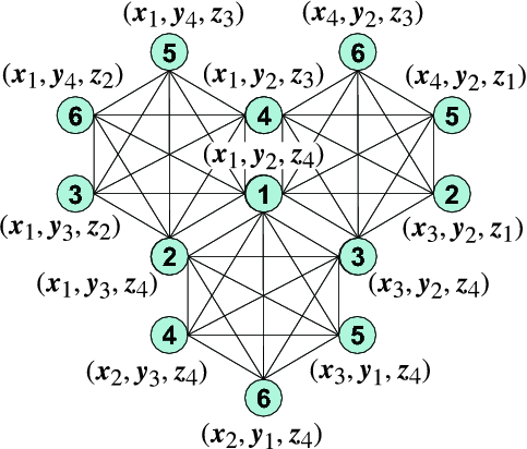
Fig. 9: (Lower right) Example of codeword assignment. Assigning a codeword to each sequence set can be regarded as vertex coloring of the coding graph.

[Encoding]

  1. 1.

    Determine a set 𝒯n​(R)⊆𝒫n​(𝒳(ℐNs))\mathcal{T}_{n}(R)\subseteq\mathcal{P}_{n}(\mathcal{X}^{(\mathcal{I}_{N_{s}})}) of joint types as

    𝒯n(R)={Q𝑿∈𝒫n(𝒳(ℐNs)):\displaystyle\mathcal{T}_{n}(R)=\{Q_{\boldsymbol{X}}\in\mathcal{P}_{n}(\mathcal{X}^{(\mathcal{I}_{N_{s}})}):
    maxj∈ℐNd⁡{H⁡(Vj|Qj)}≤R,Q𝑿=Qj​Vj,\displaystyle\hskip-14.22636pt\max_{j\in\mathcal{I}_{N_{d}}}\{H(V_{j}|Q_{j})\}\leq R,\quad Q_{\boldsymbol{X}}=Q_{j}V_{j},
    Qj∈𝒫n(𝒳(𝒮jc)),Vj∈𝒱n(𝒳(𝒮j)|Qj),∀j∈ℐNd},\displaystyle\hskip-14.22636ptQ_{j}\in\mathcal{P}_{n}(\mathcal{X}^{(\mathcal{S}_{j}^{c})}),V_{j}\in\mathcal{V}_{n}(\mathcal{X}^{(\mathcal{S}_{j})}|Q_{j}),\forall j\in\mathcal{I}_{N_{d}}\},

    where R>0R>0 is a given coding rate. We note that the joint type Q𝑿Q_{\boldsymbol{X}} and the system 𝓢\boldsymbol{\mathcal{S}} specify the type QjQ_{j} and the conditional type VjV_{j} for every j∈ℐNdj\in\mathcal{I}_{N_{d}}.

  2. 2.

    Create a graph for every joint type Q𝑿∈𝒯n​(R)Q_{\boldsymbol{X}}\in\mathcal{T}_{n}(R). An intuitive example of coding graphs is shown in Figs. 9, 9, 9 and 9, where the network shown in Fig. 5 is considered. Each vertex of the graph corresponds to a sequence set 𝒙(ℐNs)∈TQ𝑿n\boldsymbol{x}^{(\mathcal{I}_{N_{s}})}\in T_{Q_{\boldsymbol{X}}}^{n} (cf. Fig. 9). Henceforth we denote a vertex by referring to the corresponding sequence set 𝒙(ℐNs)\boldsymbol{x}^{(\mathcal{I}_{N_{s}})}. An edge is placed between vertices 𝒙1(ℐNs)\boldsymbol{x}_{1}^{(\mathcal{I}_{N_{s}})} and 𝒙2(ℐNs)\boldsymbol{x}_{2}^{(\mathcal{I}_{N_{s}})} if and only if 𝒙1(𝒮jc)=𝒙2(𝒮jc)\boldsymbol{x}_{1}^{(\mathcal{S}_{j}^{c})}=\boldsymbol{x}_{2}^{(\mathcal{S}_{j}^{c})}, 𝒙1(𝒮j)∈TVjn​(𝒙1(𝒮jc))\boldsymbol{x}_{1}^{(\mathcal{S}_{j})}\in T_{V_{j}}^{n}(\boldsymbol{x}_{1}^{(\mathcal{S}_{j}^{c})}) and 𝒙2(𝒮j)∈TVjn​(𝒙2(𝒮jc))\boldsymbol{x}_{2}^{(\mathcal{S}_{j})}\in T_{V_{j}}^{n}(\boldsymbol{x}_{2}^{(\mathcal{S}_{j}^{c})}) for some j∈ℐNdj\in\mathcal{I}_{N_{d}} (cf. Figs. 9 and 9). In the following, we call this graph the coding graph G⁡(Q𝑿)G(Q_{\boldsymbol{X}}). Note that Figs. 9 and 9 show only a subgraph that corresponds to V-shells TVjn​(𝒙(𝒮jc))T_{V_{j}}^{n}(\boldsymbol{x}^{(\mathcal{S}_{j}^{c})}), where 𝒙(𝒮1c)=𝒙1\boldsymbol{x}^{(\mathcal{S}_{1}^{c})}=\boldsymbol{x}_{1}, 𝒙(𝒮2c)=𝒚2\boldsymbol{x}^{(\mathcal{S}_{2}^{c})}=\boldsymbol{y}_{2} and 𝒙(𝒮3c)=𝒛4\boldsymbol{x}^{(\mathcal{S}_{3}^{c})}=\boldsymbol{z}_{4}.

  3. 3.

    Assign a symbol to each vertex of the coding graph G⁡(Q𝑿)G(Q_{\boldsymbol{X}}) so that the same symbol is not assigned to any pairs of adjacent vertices (cf. Fig. 9).

  4. 4.

    For an input sequence set 𝒙(ℐNs)\boldsymbol{x}^{(\mathcal{I}_{N_{s}})} whose joint type Q𝑿Q_{\boldsymbol{X}} is a member of 𝒯n​(R)\mathcal{T}_{n}(R), the index assigned to the joint type Q𝑿Q_{\boldsymbol{X}} is the first part of the codeword, and the symbol assigned to the corresponding vertex of the coding graph is determined as the second part of the codeword. For a sequence set 𝒙(ℐNs)\boldsymbol{x}^{(\mathcal{I}_{N_{s}})} whose joint type Q𝑿Q_{\boldsymbol{X}} is not a member of 𝒯n​(R)\mathcal{T}_{n}(R), the codeword is determined arbitrarily and an encoding error is declared.

[Decoding: φ^n(j)\widehat{\varphi}_{n}^{(j)}]

  1. 1.

    The first part of the received codeword represents the joint type Q^𝑿\widehat{Q}_{\boldsymbol{X}} of the input sequence. If no encoding error occurs, then Q^𝑿\widehat{Q}_{\boldsymbol{X}} should be Q𝑿Q_{\boldsymbol{X}}, and therefore the decoder φ^n(j)\widehat{\varphi}_{n}^{(j)} can find the coding graph G^​(Q^𝑿)=G⁡(Q𝑿)\widehat{G}(\widehat{Q}_{\boldsymbol{X}})=G(Q_{\boldsymbol{X}}) used in the encoding scheme.

  2. 2.

    For given side information 𝒙1(𝒮jc)\boldsymbol{x}_{1}^{(\mathcal{S}_{j}^{c})} and the joint type Q𝑿Q_{\boldsymbol{X}}, find the vertex 𝒙2(ℐNs)\boldsymbol{x}_{2}^{(\mathcal{I}_{N_{s}})} such that (i) 𝒙2(𝒮jc)=𝒙1(𝒮jc)\boldsymbol{x}_{2}^{(\mathcal{S}_{j}^{c})}=\boldsymbol{x}_{1}^{(\mathcal{S}_{j}^{c})} and (ii) the second part of the received codeword is assigned to 𝒙2(ℐNs)\boldsymbol{x}_{2}^{(\mathcal{I}_{N_{s}})}. Such a vertex is found in the clique that corresponds to the set TVjn​(𝒙(𝒮jc))T_{V_{j}}^{n}(\boldsymbol{x}^{(\mathcal{S}_{j}^{c})}). With Fig. 9, if 𝒙(𝒮1c)=𝒙1\boldsymbol{x}^{(\mathcal{S}_{1}^{c})}=\boldsymbol{x}_{1} is given as a side information sequence, we can find such a vertex from the upper left clique. Note that the conditional type VjV_{j} has been determined by Q^𝑿=Q𝑿\widehat{Q}_{\boldsymbol{X}}=Q_{\boldsymbol{X}}. The sequence set 𝒙^(𝒮j)∈TQjn\widehat{\boldsymbol{x}}^{(\mathcal{S}_{j})}\in T_{Q_{j}}^{n} found in this step is reproduced.

It should be noted that the above coding scheme is universal since it does not depend on the distribution P𝑿P_{\boldsymbol{X}} of a source 𝑿\boldsymbol{X}.

The coding rate of the above proposed coding scheme is determined by the chromatic number of the coding graph G⁡(Q𝑿)G(Q_{\boldsymbol{X}}). To this end, we introduce the following lemmas.

Lemma 7

The coding graph G⁡(Q)G(Q) of the joint type Q=Q𝐗Q=Q_{\boldsymbol{X}} has the following properties:

  1. 1.

    Every vertex set

    TVjn​(𝒙(𝒮jc))(j∈ℐNd)T_{V_{j}}^{n}(\boldsymbol{x}^{(\mathcal{S}_{j}^{c})})\quad(j\in\mathcal{I}_{N_{d}})

    comprises a clique, where

    Q=Qj​Vj,𝒙(𝒮jc)∈TQjn,\displaystyle Q=Q_{j}V_{j},\quad\boldsymbol{x}^{(\mathcal{S}_{j}^{c})}\in T_{Q_{j}}^{n},
    Qj∈𝒫n​(𝒳(𝒮jc))Vj∈𝒱n​(𝒳(𝒮j)|Qj).\displaystyle Q_{j}\in\mathcal{P}_{n}(\mathcal{X}^{(\mathcal{S}_{j}^{c})})\quad V_{j}\in\mathcal{V}_{n}(\mathcal{X}^{(\mathcal{S}_{j})}|Q_{j}).
  2. 2.

    Every vertex 𝒙(ℐNs)∈TQn\boldsymbol{x}^{(\mathcal{I}_{N_{s}})}\in T_{Q}^{n} belongs to NdN_{d} cliques, each of which corresponds to the vertex set

    TVjn​(𝒙(𝒮jc)).(j∈ℐNd)T_{V_{j}}^{n}(\boldsymbol{x}^{(\mathcal{S}_{j}^{c})}).\quad(j\in\mathcal{I}_{N_{d}})
  3. 3.

    The vertex 𝒙(ℐNs)∈TQn\boldsymbol{x}^{(\mathcal{I}_{N_{s}})}\in T_{Q}^{n} has no edges from vertices not included in the vertex sets ∪j∈ℐNdTVjn(𝒙(𝒮jc))\cup_{j\in\mathcal{I}_{N_{d}}}T_{V_{j}}^{n}(\boldsymbol{x}^{(\mathcal{S}_{j}^{c})}).

  4. 4.

    For a given joint type Q∈𝒫n​(𝒳(ℐNs))Q\in\mathcal{P}_{n}(\mathcal{X}^{(\mathcal{I}_{N_{s}})}), both the clique number ω⁡(G⁡(Q))\omega(G(Q)) and the degree Δ⁡(G⁡(Q))\Delta(G(Q)) of the coding graph G⁡(Q)G(Q) are constant and obtained as follows:

    ω⁡(G⁡(Q))\displaystyle\omega(G(Q)) =\displaystyle= maxj∈ℐNd⁡|TVjn​(𝒙(𝒮jc))|,\displaystyle\max_{j\in\mathcal{I}_{N_{d}}}|T_{V_{j}}^{n}(\boldsymbol{x}^{(\mathcal{S}_{j}^{c})})|,
    Δ⁡(G⁡(Q))\displaystyle\Delta(G(Q)) =\displaystyle= ∑j∈ℐNd|TVjn​(𝒙(𝒮jc))|.\displaystyle\sum_{j\in\mathcal{I}_{N_{d}}}|T_{V_{j}}^{n}(\boldsymbol{x}^{(\mathcal{S}_{j}^{c})})|.
Proof:

1) 2) 3) Easily obtained from the first and second steps of the above encoding scheme. 4) Easily obtained from the above properties. ∎

Lemma 8

The chromatic number of the coding graph G⁡(Q)G(Q) of the joint type Q∈𝒯n​(R)Q\in\mathcal{T}_{n}(R) is bounded as

χ⁡(G⁡(Q))\displaystyle\chi(G(Q)) ≤\displaystyle\leq Nd​exp⁡(n​R).\displaystyle N_{d}\exp(nR).
Proof:

This property is directly derived from Lemmas 2, 4 and 7 as follows:

χ⁡(G⁡(Q))\displaystyle\chi(G(Q)) ≤\displaystyle\leq Δ⁡(G⁡(Q))\displaystyle\Delta(G(Q)) (1)
=\displaystyle= ∑j∈ℐNd|TVjn​(𝒙(𝒮jc))|\displaystyle\sum_{j\in\mathcal{I}_{N_{d}}}|T_{V_{j}}^{n}(\boldsymbol{x}^{(\mathcal{S}_{j}^{c})})| (2)
≤\displaystyle\leq ∑j∈ℐNdexp⁡{n​H​(Vj|Qj)}\displaystyle\sum_{j\in\mathcal{I}_{N_{d}}}\exp\{nH(V_{j}|Q_{j})\} (3)
≤\displaystyle\leq Nd​exp⁡{n​maxj∈ℐNd⁡H⁡(Vj|Qj)}\displaystyle N_{d}\exp\{n\max_{j\in\mathcal{I}_{N_{d}}}H(V_{j}|Q_{j})\}
≤\displaystyle\leq Nd​exp⁡(n​R).\displaystyle N_{d}\exp(nR). (4)

where Eq. (1) comes from Lemma 4, Eq. (2) from Lemma 7, Eq. (3) from Lemma 2, and Eq. (4) from the definition of 𝒯n​(R)\mathcal{T}_{n}(R). This concludes the proof of Lemma 8. ∎

From the above discussions, we obtain

ω⁡(G⁡(Q))≤χ⁡(G⁡(Q))≤Δ⁡(G⁡(Q))≤Nd​exp⁡(n​R).\omega(G(Q))\leq\chi(G(Q))\leq\Delta(G(Q))\leq N_{d}\exp(nR).

V Coding theorems

V-A General cases

We show several coding theorems derived from the proposed coding scheme. Before showing these coding theorems, let us define the following function:

ϵn​(N)\displaystyle\epsilon_{n}(N) =def.\displaystyle{\displaystyle\mathop{=}^{\mbox{\rm def.}}} 1n​{|𝒳(ℐNs)|​log⁡(n+1)+log⁡N}\displaystyle\frac{1}{n}\{|\mathcal{X}^{(\mathcal{I}_{N_{s}})}|\log(n+1)+\log N\} (5)
→\displaystyle\to 0(n→∞).\displaystyle 0\quad(n\to\infty).

First we present the direct part of the coding theorem for the universal FF-GCD codes, which implies that the coding scheme shown in Section IV attains the minimum achievable rate.

Theorem 3

For a given real number R>0R>0, there exists a universal FF-GCD code

{(φn,φ^n(1),⋯,φ^n(Nd))}n=1∞\{(\varphi_{n},\widehat{\varphi}_{n}^{(1)},\cdots,\widehat{\varphi}_{n}^{(N_{d})})\}_{n=1}^{\infty}

for the network 𝓢\boldsymbol{\mathcal{S}} such that for any integer n≥1n\geq 1 and any source 𝐗\boldsymbol{X}

1n​log⁡Mn\displaystyle\frac{1}{n}\log M_{n} ≤\displaystyle\leq R+ϵn​(Nd),\displaystyle R+\epsilon_{n}(N_{d}), (6)
∑j=1Nden(j)\displaystyle\sum_{j=1}^{N_{d}}e_{n}^{(j)} ≤\displaystyle\leq
exp{−n(−ϵn(Nd)+minQ𝑿∈𝒯nc​(R)D(Q𝑿∥P𝑿))}.\displaystyle\hskip-45.5244pt\exp\left\{-n\left(-\epsilon_{n}(N_{d})+\hskip-5.69054pt\min_{Q_{\boldsymbol{X}}\in\mathcal{T}_{n}^{c}(R)}\hskip-5.69054ptD(Q_{\boldsymbol{X}}\|P_{\boldsymbol{X}})\right)\right\}.
Proof:

Note that a codeword is composed of two parts: the first part corresponds to the joint type of an input sequence set, and the second part represents a symbol assigned to the input sequence set in the coding graph of the joint type. Therefore, the size of the codeword set is bounded as

Mn\displaystyle M_{n} ≤\displaystyle\leq |𝒫n​(𝒳(ℐNs))|⋅Nd​exp⁡(n​R)\displaystyle|\mathcal{P}_{n}(\mathcal{X}^{(\mathcal{I}_{N_{s}})})|\cdot N_{d}\exp(nR)
≤\displaystyle\leq Nd​(n+1)|𝒳(ℐNs)|​exp⁡(n​R),(Lemma 1)\displaystyle N_{d}(n+1)^{|\mathcal{X}^{(\mathcal{I}_{N_{s}})}|}\exp(nR),\quad(\mbox{Lemma \ref{lemma:typecount}})

which implies Eq. (6). Next, we evaluate decoding error probabilities. Since every sequence set 𝒙(ℐNs)​n\boldsymbol{x}^{(\mathcal{I}_{N_{s}})n} whose joint type is a member of 𝒯n​(R)\mathcal{T}_{n}(R) is reproduced correctly at the decoder, the sum of the error probabilities is bounded as

∑j=1Nden(j)\displaystyle\sum_{j=1}^{N_{d}}e_{n}^{(j)} (7)
≤\displaystyle\leq Nd​Pr⁡{𝑿n∈TQ~𝑿n:Q~𝑿∈𝒯nc​(R)}\displaystyle N_{d}\Pr\left\{\boldsymbol{X}^{n}\in T_{\widetilde{Q}_{\boldsymbol{X}}}^{n}:\widetilde{Q}_{\boldsymbol{X}}\in\mathcal{T}_{n}^{c}(R)\right\}
≤\displaystyle\leq Nd∑Q~𝑿∈𝒯nc​(R)exp{−nD(Q~𝑿∥P𝑿)}\displaystyle N_{d}\sum_{\widetilde{Q}_{\boldsymbol{X}}\in\mathcal{T}_{n}^{c}(R)}\exp\{-nD(\widetilde{Q}_{\boldsymbol{X}}\|P_{\boldsymbol{X}})\} (8)
≤\displaystyle\leq Nd∑Q~𝑿∈𝒯nc​(R)exp{−nminQ𝑿∈𝒯nc​(R)D(Q𝑿∥P𝑿)}\displaystyle N_{d}\sum_{\widetilde{Q}_{\boldsymbol{X}}\in\mathcal{T}_{n}^{c}(R)}\hskip-11.38109pt\exp\left\{-n\min_{Q_{\boldsymbol{X}}\in\mathcal{T}_{n}^{c}(R)}D(Q_{\boldsymbol{X}}\|P_{\boldsymbol{X}})\right\}
≤\displaystyle\leq Nd​(n+1)|𝒳(ℐNs)|\displaystyle N_{d}(n+1)^{|\mathcal{X}^{(\mathcal{I}_{N_{s}})}|}
×exp{−nminQ𝑿∈𝒯nc​(R)D(Q𝑿∥P𝑿)}\displaystyle\hskip 28.45274pt\times\exp\left\{-n\min_{Q_{\boldsymbol{X}}\in\mathcal{T}_{n}^{c}(R)}D(Q_{\boldsymbol{X}}\|P_{\boldsymbol{X}})\right\} (9)
=\displaystyle= exp{−n(−ϵn(Nd)+minQ𝑿∈𝒯nc​(R)D(Q𝑿∥P𝑿))},\displaystyle\exp\left\{-n\left(-\epsilon_{n}(N_{d})+\hskip-5.69054pt\min_{Q_{\boldsymbol{X}}\in\mathcal{T}_{n}^{c}(R)}D(Q_{\boldsymbol{X}}\|P_{\boldsymbol{X}})\right)\right\},

where Eq. (8) comes from Lemma 3, and Eq. (9) from Lemma 1. This completes the proof of Theorem 3. ∎

We can see that for any real value R≥Rf​(𝑿|𝓢)R\geq R_{f}(\boldsymbol{X}|\boldsymbol{\mathcal{S}}) we have

minQ𝑿∈𝒯nc​(R)D(Q𝑿∥P𝑿)\displaystyle\min_{Q_{\boldsymbol{X}}\in\mathcal{T}_{n}^{c}(R)}D(Q_{\boldsymbol{X}}\|P_{\boldsymbol{X}}) >\displaystyle> 0.\displaystyle 0.

This implies that if R≥Rf​(𝑿|𝓢)R\geq R_{f}(\boldsymbol{X}|\boldsymbol{\mathcal{S}}) there exists an FF-GCD code for the network 𝓢\boldsymbol{\mathcal{S}} that universally attains the conditions shown in Definition 2.

The following converse theorem indicates that the error exponent obtained in Theorem 3 is tight.

Theorem 4

Any FF-GCD code

{(φn,φ^n(1),⋯,φ^n(Nd))}n=1∞\{(\varphi_{n},\widehat{\varphi}_{n}^{(1)},\cdots,\widehat{\varphi}_{n}^{(N_{d})})\}_{n=1}^{\infty}

for the system 𝓢\boldsymbol{\mathcal{S}} must satisfy

∑j=1Nden(j)\displaystyle\sum_{j=1}^{N_{d}}e_{n}^{(j)}
≥\displaystyle\geq exp{−n(ϵn(2)+minQ𝑿∈𝒯nc​(R+ϵn​(2))D(Q𝑿∥P𝑿))}\displaystyle\exp\left\{-n\left(\epsilon_{n}(2)+\hskip-5.69054pt\min_{Q_{\boldsymbol{X}}\in\mathcal{T}_{n}^{c}(R+\epsilon_{n}(2))}D(Q_{\boldsymbol{X}}\|P_{\boldsymbol{X}})\right)\right\}

for any integer n≥1n\geq 1, any source 𝐗\boldsymbol{X} and a given coding rate R=1/n​log⁡Mn>0R=1/n\log M_{n}>0.

Proof:

Note that the number of sequences to be decoded correctly for each decoder is at most exp⁡(n​R)\exp(nR). Here, let us consider a joint type Q𝑿∈𝒯nc​(R+ϵn​(2))Q_{\boldsymbol{X}}\in\mathcal{T}_{n}^{c}(R+\epsilon_{n}(2)). The definition of 𝒯nc​(R+ϵn​(2))\mathcal{T}_{n}^{c}(R+\epsilon_{n}(2)) and Lemma 2 imply that for 𝒙(ℐNs)∈TQ𝑿n\boldsymbol{x}^{(\mathcal{I}_{N_{s}})}\in T_{Q_{\boldsymbol{X}}}^{n} we have

maxj∈ℐNd⁡{|TVjn​(𝒙(𝒮jc))|}\displaystyle\max_{j\in\mathcal{I}_{N_{d}}}\{|T_{V_{j}}^{n}(\boldsymbol{x}^{(\mathcal{S}_{j}^{c})})|\} (10)
≥\displaystyle\geq (n+1)−|𝒳(ℐNs)|​maxj∈ℐNd​exp⁡{n​H​(Vj|Qj)}\displaystyle(n+1)^{-|\mathcal{X}^{(\mathcal{I}_{N_{s}})}|}\max_{j\in\mathcal{I}_{N_{d}}}\exp\{nH(V_{j}|Q_{j})\}
≥\displaystyle\geq (n+1)−|𝒳(ℐNs)|​exp⁡{n⁡(R+ϵn​(2))}\displaystyle(n+1)^{-|\mathcal{X}^{(\mathcal{I}_{N_{s}})}|}\exp\{n(R+\epsilon_{n}(2))\} (11)
=\displaystyle= 2​exp⁡(n​R),\displaystyle 2\exp(nR),

where Eq. (10) comes from Lemma 2, and Eq. (11) from the definition of 𝒯nc​(R+ϵn​(2))\mathcal{T}_{n}^{c}(R+\epsilon_{n}(2)). Therefore, at least half of the sequence sets in TQ𝑿nT_{Q_{\boldsymbol{X}}}^{n} will not be decoded correctly at the decoder φ^n(j)\widehat{\varphi}_{n}^{(j)}. Thus, the sum of the error probabilities is bounded as

∑j∈ℐNden(j)\displaystyle\sum_{j\in\mathcal{I}_{N_{d}}}e_{n}^{(j)}
≥\displaystyle\geq 12∑Q𝑿∈𝒯nc​(R+ϵn​(2))Pr{𝑿n∈TQ𝑿n}\displaystyle\frac{1}{2}\sum_{Q_{\boldsymbol{X}}\in\mathcal{T}_{n}^{c}(R+\epsilon_{n}(2))}\Pr\{\boldsymbol{X}^{n}\in T_{Q_{\boldsymbol{X}}}^{n}\}
≥\displaystyle\geq 12(n+1)−|𝒳(ℐNs)|∑Q𝑿∈𝒯nc​(R+ϵn​(2))exp{−nD(Q𝑿∥P𝑿)}\displaystyle\frac{1}{2}(n+1)^{-|\mathcal{X}^{(\mathcal{I}_{N_{s}})}|}\hskip-14.22636pt\sum_{Q_{\boldsymbol{X}}\in\mathcal{T}_{n}^{c}(R+\epsilon_{n}(2))}\hskip-14.22636pt\exp\{-nD(Q_{\boldsymbol{X}}\|P_{\boldsymbol{X}})\}
≥\displaystyle\geq 12​(n+1)−|𝒳(ℐNs)|\displaystyle\frac{1}{2}(n+1)^{-|\mathcal{X}^{(\mathcal{I}_{N_{s}})}|}
×exp{−nminQ𝑿∈𝒯nc​(R+ϵn​(2))D(Q𝑿∥P𝑿)}\displaystyle\times\exp\left\{-n\hskip-5.69054pt\min_{Q_{\boldsymbol{X}}\in\mathcal{T}_{n}^{c}(R+\epsilon_{n}(2))}\hskip-5.69054ptD(Q_{\boldsymbol{X}}\|P_{\boldsymbol{X}})\right\}
=\displaystyle= exp{−n(ϵn(2)+minQ𝑿∈𝒯nc​(R+ϵn​(2))D(Q𝑿∥P𝑿))},\displaystyle\exp\left\{-n\left(\epsilon_{n}(2)+\hskip-5.69054pt\min_{Q_{\boldsymbol{X}}\in\mathcal{T}_{n}^{c}(R+\epsilon_{n}(2))}D(Q_{\boldsymbol{X}}\|P_{\boldsymbol{X}})\right)\right\},

where Eq. () comes from Lemma 3. This concludes the proof of Theorem 4. ∎

The following corollary is directly derived from Theorems 3 and 4. This shows the asymptotic optimality of the proposed coding scheme.

Corollary 1

For a given real number R>0R>0, there exists a universal FF-GCD code

{(φn,φ^n(1),⋯,φ^n(Nd))}n=1∞\{(\varphi_{n},\widehat{\varphi}_{n}^{(1)},\cdots,\widehat{\varphi}_{n}^{(N_{d})})\}_{n=1}^{\infty}

for the network 𝓢\boldsymbol{\mathcal{S}} such that for any source 𝐗\boldsymbol{X}

lim supn→∞1n​log⁡Mn≤R,\displaystyle\limsup_{n\to\infty}\frac{1}{n}\log M_{n}\leq R,
limn→∞−1nlog∑j∈ℐNden(j)=minQ𝑿∈𝒯c​(R)D(Q𝑿∥P𝑿),\displaystyle\lim_{n\to\infty}-\frac{1}{n}\log\sum_{j\in\mathcal{I}_{N_{d}}}e_{n}^{(j)}=\min_{Q_{\boldsymbol{X}}\in\mathcal{T}^{c}(R)}D(Q_{\boldsymbol{X}}\|P_{\boldsymbol{X}}),

where

𝒯(R)={Q𝑿∈𝒫(𝒳(ℐNs)):\displaystyle\mathcal{T}(R)=\{Q_{\boldsymbol{X}}\in\mathcal{P}(\mathcal{X}^{(\mathcal{I}_{N_{s}})}):
maxj∈ℐNd⁡H⁡(Vj|Qj)≤R,Q𝑿=Qj​Vj,\displaystyle\hskip 5.69054pt\max_{j\in\mathcal{I}_{N_{d}}}H(V_{j}|Q_{j})\leq R,\quad Q_{\boldsymbol{X}}=Q_{j}V_{j},
Qj∈𝒫n(𝒳(𝒮jc)),Vj∈𝒱(𝒳(𝒮j)|Qj),∀j∈ℐNd}.\displaystyle\hskip 5.69054ptQ_{j}\in\mathcal{P}_{n}(\mathcal{X}^{(\mathcal{S}_{j}^{c})}),V_{j}\in\mathcal{V}(\mathcal{X}^{(\mathcal{S}_{j})}|Q_{j}),\forall j\in\mathcal{I}_{N_{d}}\}.

In a similar manner, we can obtain a probability such that the original sequence set is correctly reproduced. The following theorem shows the lower bound of the probability of correct decoding that can be achieved by the proposed coding scheme.

Theorem 5

For a given real number R>0R>0, there exists a universal FF-GCD code

{(φn,φ^n(1),⋯,φ^n(Nd))}n=1∞\{(\varphi_{n},\widehat{\varphi}_{n}^{(1)},\cdots,\widehat{\varphi}_{n}^{(N_{d})})\}_{n=1}^{\infty}

for the network 𝓢\boldsymbol{\mathcal{S}} such that for any integer n≥1n\geq 1 and any source 𝐗\boldsymbol{X}

1n​log⁡Mn\displaystyle\frac{1}{n}\log M_{n} ≤\displaystyle\leq R+ϵn​(Nd),\displaystyle R+\epsilon_{n}(N_{d}), (13)
1−∑j=1Nden(j)\displaystyle 1-\sum_{j=1}^{N_{d}}e_{n}^{(j)} ≥\displaystyle\geq
exp{−n(ϵn(1)+minQ𝑿∈𝒯n​(R)D(Q𝑿∥P𝑿))}.\displaystyle\hskip-36.98857pt\exp\left\{-n\left(\epsilon_{n}(1)+\min_{Q_{\boldsymbol{X}}\in\mathcal{T}_{n}(R)}D(Q_{\boldsymbol{X}}\|P_{\boldsymbol{X}})\right)\right\}.
Proof:

Eq. (13) is derived in the same way as the proof of Theorem 3. Next, we evaluate the probability such that the original sequence set is correctly reproduced. Since every sequence set 𝒙(ℐNs)\boldsymbol{x}^{(\mathcal{I}_{N_{s}})} whose joint type is a member of 𝒯n​(R)\mathcal{T}_{n}(R) is reproduced correctly at the decoder, the sum of the probabilities is bounded as

1−∑j=1Nden(j)\displaystyle 1-\sum_{j=1}^{N_{d}}e_{n}^{(j)}
≥\displaystyle\geq Pr⁡{𝑿n∈TQ𝑿n:Q𝑿∈𝒯n​(R)}\displaystyle\Pr\left\{\boldsymbol{X}^{n}\in T_{Q_{\boldsymbol{X}}}^{n}:Q_{\boldsymbol{X}}\in\mathcal{T}_{n}(R)\right\}
≥\displaystyle\geq ∑Q𝑿∈𝒯n​(R)(n+1)−|𝒳(ℐNs)|exp{−nD(Q𝑿∥P𝑿)}\displaystyle\sum_{Q_{\boldsymbol{X}}\in\mathcal{T}^{n}(R)}\hskip-11.38109pt(n+1)^{-|\mathcal{X}^{(\mathcal{I}_{N_{s}})}|}\exp\{-nD(Q_{\boldsymbol{X}}\|P_{\boldsymbol{X}})\}
≥\displaystyle\geq (n+1)−|𝒳(ℐNs)|\displaystyle(n+1)^{-|\mathcal{X}^{(\mathcal{I}_{N_{s}})}|}
×exp{−nminQ𝑿∈𝒯n​(R)D(Q𝑿∥P𝑿)}\displaystyle\times\exp\left\{-n\min_{Q_{\boldsymbol{X}}\in\mathcal{T}^{n}(R)}D(Q_{\boldsymbol{X}}\|P_{\boldsymbol{X}})\right\}
=\displaystyle= exp{−n(ϵn(1)+minQ𝑿∈𝒯n​(R)D(Q𝑿∥P𝑿))},\displaystyle\exp\left\{-n\left(\epsilon_{n}(1)+\min_{Q_{\boldsymbol{X}}\in\mathcal{T}_{n}(R)}D(Q_{\boldsymbol{X}}\|P_{\boldsymbol{X}})\right)\right\},

where Eq. () comes from Lemma 3. This completes the proof of Theorem 5. ∎

The following converse theorem indicates that the exponent of correct decoding obtained in Theorem 5 might not be tight.

Theorem 6

Any FF-GCD code

{(φn,φ^n(1),⋯,φ^n(Nd))}n=1∞\{(\varphi_{n},\widehat{\varphi}_{n}^{(1)},\cdots,\widehat{\varphi}_{n}^{(N_{d})})\}_{n=1}^{\infty}

for the network 𝓢\boldsymbol{\mathcal{S}} must satisfy

1−∑j=1Nden(j)≤exp[−n{−ϵn(1)+minQ𝑿∈𝒫n​(𝒳(ℐNs))\displaystyle 1-\sum_{j=1}^{N_{d}}e_{n}^{(j)}\leq\exp\Bigl[-n\Bigl\{-\epsilon_{n}(1)+\min_{Q_{\boldsymbol{X}}\in\mathcal{P}_{n}(\mathcal{X}^{(\mathcal{I}_{N_{s}})})}
(|maxj∈ℐNdH(Vj|Qj)−(R+ϵn(1))|++D(Q𝑿∥P𝑿))}]\displaystyle\hskip-8.53581pt\left(\left|\max_{j\in\mathcal{I}_{N_{d}}}H(V_{j}|Q_{j})-(R+\epsilon_{n}(1))\right|^{+}+D(Q_{\boldsymbol{X}}\|P_{\boldsymbol{X}})\right)\Biggr\}\Biggr]

for any integer n≥1n\geq 1, any source 𝐗\boldsymbol{X} and a given coding rate R=1/n​log⁡Mn>0R=1/n\log M_{n}>0, where

Q𝑿=Qj​Vj,∀j∈ℐNdQj∈𝒫n​(𝒳(𝒮jc)),Vj∈𝒱⁡(𝒳(𝒮j)|Qj)}\displaystyle\left.\begin{array}[]{l}Q_{\boldsymbol{X}}=Q_{j}V_{j},\quad\forall j\in\mathcal{I}_{N_{d}}\\ Q_{j}\in\mathcal{P}_{n}(\mathcal{X}^{(\mathcal{S}_{j}^{c})}),\quad V_{j}\in\mathcal{V}(\mathcal{X}^{(\mathcal{S}_{j})}|Q_{j})\end{array}\right\}

and |a|+=max⁡{a,0}|a|^{+}=\max\{a,0\}.

Proof:

Note that the number of sequences to be decoded correctly for each decoder is at most exp⁡(n​R)\exp(nR). Here, let us consider Q𝑿∈𝒫n​(𝒳(ℐNs))Q_{\boldsymbol{X}}\in\mathcal{P}_{n}(\mathcal{X}^{(\mathcal{I}_{N_{s}})}), QjQ_{j} and VjV_{j} that satisfy Eq. (6). The ratio rc​(Q𝑿)r_{c}(Q_{\boldsymbol{X}}) of sequences in the sequence set TQ𝑿T_{Q_{\boldsymbol{X}}} that the sequences are correctly reproduced is at most

rc​(Q𝑿)\displaystyle r_{c}(Q_{\boldsymbol{X}}) (18)
≤\displaystyle\leq min⁡{minj∈ℐNd⁡(exp⁡(n​R)|TVjn​(𝒙(𝒮jc))|),1}\displaystyle\min\left\{\min_{j\in\mathcal{I}_{N_{d}}}\left(\frac{\exp(nR)}{|T_{V_{j}}^{n}(\boldsymbol{x}^{(\mathcal{S}_{j}^{c})})|}\right),1\right\}
≤\displaystyle\leq min[exp(nR)⋅(n+1)|𝒳(ℐNs)|\displaystyle\min\Bigl[\exp(nR)\cdot(n+1)^{|\mathcal{X}^{(\mathcal{I}_{N_{s}})}|}
×exp{−nmaxj∈ℐNdH(Vj|Qj)},1]\displaystyle\hskip 17.07164pt\times\exp\{-n\max_{j\in\mathcal{I}_{N_{d}}}H(V_{j}|Q_{j})\},1\Bigr]
=\displaystyle= min[exp{−n{maxj∈ℐNdH(Vj|Qj)−(R+ϵn(1))},1]\displaystyle\min\Bigl[\exp\{-n\{\max_{j\in\mathcal{I}_{N_{d}}}H(V_{j}|Q_{j})-(R+\epsilon_{n}(1))\},1\Bigr]
=\displaystyle= exp⁡{−n​|maxj∈ℐNd⁡H⁡(Vj|Qj)−(R+ϵn​(1))|+},\displaystyle\exp\left\{-n\left|\max_{j\in\mathcal{I}_{N_{d}}}H(V_{j}|Q_{j})-\left(R+\epsilon_{n}(1)\right)\right|^{+}\right\},

where Eq. (18) comes from Lemma 2. Therefore, the probability Pc​(Q𝑿)P_{c}(Q_{\boldsymbol{X}}) such that the original sequence pair with type Q𝑿Q_{\boldsymbol{X}} is correctly reproduced is bounded as

Pc​(Q𝑿)\displaystyle P_{c}(Q_{\boldsymbol{X}}) (19)
≤\displaystyle\leq rc(Q𝑿)Pr{𝑿n∈TQ𝑿n}\displaystyle r_{c}(Q_{\boldsymbol{X}})\Pr\{\boldsymbol{X}^{n}\in T_{Q_{\boldsymbol{X}}}^{n}\}
≤\displaystyle\leq exp{−n|maxj∈ℐNdH(Vj|Qj)−(R+ϵn(1))|+\displaystyle\exp\bigl\{-n\bigl|\max_{j\in\mathcal{I}_{N_{d}}}H(V_{j}|Q_{j})-\left(R+\epsilon_{n}(1)\right)\bigr|^{+}
+D(Q𝑿∥P𝑿)},\displaystyle\hskip 28.45274pt+D(Q_{\boldsymbol{X}}\|P_{\boldsymbol{X}})\bigr\},

where Eq. (19) comes from Lemma 3. Thus, the sum of the probabilities of correct decoding is obtained as

1−∑j=1Nden(j)\displaystyle 1-\sum_{j=1}^{N_{d}}e_{n}^{(j)}
≤\displaystyle\leq ∑Q𝑿∈𝒫n​(𝒳(ℐNs))Pc​(Q𝑿)\displaystyle\sum_{Q_{\boldsymbol{X}}\in\mathcal{P}_{n}(\mathcal{X}^{(\mathcal{I}_{N_{s}})})}P_{c}(Q_{\boldsymbol{X}})
≤\displaystyle\leq ∑Q𝑿∈𝒫n​(𝒳(ℐNs))exp{−n|maxj∈ℐNdH(Vj|Qj)\displaystyle\sum_{Q_{\boldsymbol{X}}\in\mathcal{P}_{n}(\mathcal{X}^{(\mathcal{I}_{N_{s}})})}\hskip-17.07164pt\exp\bigl\{-n\bigl|\max_{j\in\mathcal{I}_{N_{d}}}H(V_{j}|Q_{j})
−(R+ϵn(1))|++D(Q𝑿∥P𝑿)}\displaystyle\hskip 28.45274pt-\left(R+\epsilon_{n}(1)\right)\bigr|^{+}+D(Q_{\boldsymbol{X}}\|P_{\boldsymbol{X}})\bigr\}
≤\displaystyle\leq (n+1)|𝒳(ℐNs)|exp{−nminQ𝑿∈𝒫n​(𝒳(ℐNs))\displaystyle(n+1)^{|\mathcal{X}^{(\mathcal{I}_{N_{s}})}|}\exp\bigl\{-n\min_{Q_{\boldsymbol{X}}\in\mathcal{P}_{n}(\mathcal{X}^{(\mathcal{I}_{N_{s}})})}
(|maxj∈ℐNdH(Vj|Qj)−(R+ϵn(1))|++D(Q𝑿∥P𝑿))},\displaystyle\hskip-14.22636pt\Bigl(\Bigl|\max_{j\in\mathcal{I}_{N_{d}}}H(V_{j}|Q_{j})-\left(R+\epsilon_{n}(1)\right)\Bigr|^{+}+D(Q_{\boldsymbol{X}}\|P_{\boldsymbol{X}})\Bigr)\Bigr\},
=\displaystyle= exp[−n{−ϵn(1)+minQ𝑿∈𝒫n​(𝒳(ℐNs))\displaystyle\exp\Bigl[-n\Bigl\{-\epsilon_{n}(1)+\min_{Q_{\boldsymbol{X}}\in\mathcal{P}_{n}(\mathcal{X}^{(\mathcal{I}_{N_{s}})})}
(|maxj∈ℐNdH(Vj|Qj)−(R+ϵn(1))|++D(Q𝑿∥P𝑿))}]\displaystyle\hskip-14.22636pt\Bigl(\Bigl|\max_{j\in\mathcal{I}_{N_{d}}}H(V_{j}|Q_{j})-\left(R+\epsilon_{n}(1)\right)\Bigr|^{+}+D(Q_{\boldsymbol{X}}\|P_{\boldsymbol{X}})\Bigr)\Bigr\}\Bigr]

where Eq. () comes from Lemma 1. This completes the proof of Theorem 6. ∎

We can see that for any real value R≥Rf​(𝑿|𝓢)R\geq R_{f}(\boldsymbol{X}|\boldsymbol{\mathcal{S}}) and sufficiently large nn we have

minQ𝑿∈𝒫⁡(𝒳(ℐNs))⁡(|maxj∈ℐNd⁡H⁡(Vj|Qj)−R|+CLOSE\displaystyle\min_{Q_{\boldsymbol{X}}\in\mathcal{P}(\mathcal{X}^{(\mathcal{I}_{N_{s}})})}\Bigl(\Bigl|\max_{j\in\mathcal{I}_{N_{d}}}H(V_{j}|Q_{j})-R\bigr|^{+}
+D(Q𝑿∥P𝑿))}\displaystyle\hskip 28.45274pt+D(Q_{\boldsymbol{X}}\|P_{\boldsymbol{X}})\bigr)\bigr\}
=\displaystyle= |maxj∈ℐNd⁡H⁡(P𝑿(𝒮j)|𝑿(𝒮jc)|P𝑿(𝒮jc))−R|+\displaystyle\left|\max_{j\in\mathcal{I}_{N_{d}}}H\left(P_{\boldsymbol{X}^{(\mathcal{S}_{j})}|\boldsymbol{X}^{(\mathcal{S}_{j}^{c})}}|P_{\boldsymbol{X}^{(\mathcal{S}_{j}^{c})}}\right)-R\right|^{+}
=\displaystyle= 0.\displaystyle 0.

On the other hand, for any real value R<Rf​(𝑿|𝓢)R<R_{f}(\boldsymbol{X}|\boldsymbol{\mathcal{S}}) we have

minQ𝑿∈𝒯⁡(R)D(Q𝑿∥P𝑿)\displaystyle\min_{Q_{\boldsymbol{X}}\in\mathcal{T}(R)}D(Q_{\boldsymbol{X}}\|P_{\boldsymbol{X}})
≥\displaystyle\geq minQ𝑿∈𝒫⁡(𝒳(ℐNs))⁡(|maxj∈ℐNd⁡H⁡(Vj|Qj)−R|+CLOSE\displaystyle\min_{Q_{\boldsymbol{X}}\in\mathcal{P}(\mathcal{X}^{(\mathcal{I}_{N_{s}})})}\bigl(\bigl|\max_{j\in\mathcal{I}_{N_{d}}}H(V_{j}|Q_{j})-R\bigr|^{+}
+D(Q𝑿∥P𝑿))}\displaystyle\hskip 56.9055pt+D(Q_{\boldsymbol{X}}\|P_{\boldsymbol{X}})\bigr)\bigr\}
≥\displaystyle\geq 0.\displaystyle 0.

This implies that the exponent of correct decoding obtained in Theorem 5 might not be tight.

Remark 2

The proof of the achievability part in the paper by Willems et al. [12] implies that any (universal) Slepian-Wolf code can be directly utilized as a (universal) FF-GCD code. Namely, the Slepian-Wolf code is achievable as an FF-GCD code if its coding rate satisfies R≥Rf​(𝐗|𝓢)R\geq R_{f}(\boldsymbol{X}|\boldsymbol{\mathcal{S}}). However, such coding schemes cannot attain the optimal error exponent shown in Theorem 4, since any existing construction of universal Slepian-Wolf codes cannot attain the optimal error exponent. On the other hand, the coding scheme presented in Section IV can attain the optimal error exponent as shown in Theorem 3.

V-B Some special cases

Here, let us consider a special case where the number of decoders equals Nd=2N_{d}=2. One of the most representative examples is the (original) complementary delivery network, where Ns=Nd=2N_{s}=N_{d}=2, 𝒮1={1}\mathcal{S}_{1}=\{1\} and 𝒮2={2}\mathcal{S}_{2}=\{2\}. We have proposed a universal coding scheme for the complementary delivery network [26, 27], where we utilized a bipartite graph as a codebook. The following of this subsection discusses the relationships between the previous coding scheme and the new coding scheme shown in Section IV.

With Nd=2N_{d}=2, the coding graph G⁡(Q)G(Q) can be translated into an equivalent bipartite graph (denoted by G~​(Q)\widetilde{G}(Q)) such that

  • •

    each vertex in one set corresponds to a sequence 𝒙(𝒮1c)∈TQ1n\boldsymbol{x}^{(\mathcal{S}_{1}^{c})}\in T_{Q_{1}}^{n}, and each vertex in the other set corresponds to a sequence 𝒙(𝒮2c)∈TQ2n\boldsymbol{x}^{(\mathcal{S}_{2}^{c})}\in T_{Q_{2}}^{n}.

  • •

    each edge corresponds to a sequence set 𝒙(ℐNs)∈TQn\boldsymbol{x}^{(\mathcal{I}_{N_{s}})}\in T_{Q}^{n}, and the edge links between two vertices, each of which corresponds to the sequence subset 𝒙(𝒮jc)∈TQjn\boldsymbol{x}^{(\mathcal{S}_{j}^{c})}\in T_{Q_{j}}^{n} (j=1,2)(j=1,2) of the sequence set 𝒙(ℐNs)\boldsymbol{x}^{(\mathcal{I}_{N_{s}})}.

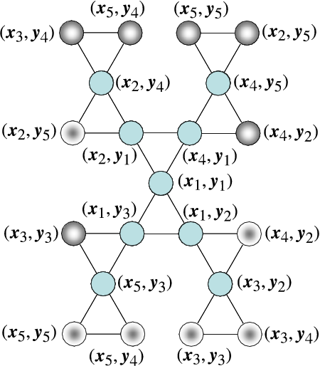
Refer to caption
Fig. 10: Example of the coding graph when Nd=2N_{d}=2, where each vertex with a gray center corresponds to another vertex with a gray verge. For example, the vertex (𝒙3,𝒚4)(\boldsymbol{x}_{3},\boldsymbol{y}_{4}) exists at the top left and the bottom right.
Refer to caption
Fig. 11: Bipartite graph equivalent to the coding graph shown in Fig. 10

Fig. 11 shows an example of bipartite graphs equivalent to the coding graph shown in Fig. 10.

From the nature of the equivalent bipartite graph G~​(Q)\widetilde{G}(Q), we can easily obtain

χ⁡(G)\displaystyle\chi(G) =\displaystyle= χ′​(G~).\displaystyle\chi^{\prime}(\widetilde{G}).

Therefore, the coding rate of the proposed coding scheme is determined by the edge chromatic number χ′​(G~)\chi^{\prime}(\widetilde{G}) of the equivalent bipartite graph G~​(Q)\widetilde{G}(Q). To this end, we introduce the following lemmas.

Lemma 9

If the number of decoders equals Nd=2N_{d}=2, then the degree of the bipartite graph G~​(Q)\widetilde{G}(Q) equivalent to the coding graph G⁡(Q)G(Q) is constant for a given joint type Q∈𝒫n​(𝒳(ℐNs))Q\in\mathcal{P}_{n}(\mathcal{X}^{(\mathcal{I}_{N_{s}})}), obtained as follows:

Δ​(G~​(Q))\displaystyle\Delta(\widetilde{G}(Q)) =\displaystyle= maxj=1,2⁡|TVjn​(𝒙(𝒮jc))|,\displaystyle\max_{j=1,2}|T_{V_{j}}^{n}(\boldsymbol{x}^{(\mathcal{S}_{j}^{c})})|,

where 𝐱(𝒮jc)∈TQjn\boldsymbol{x}^{(\mathcal{S}_{j}^{c})}\in T_{Q_{j}}^{n}. This equals the clique number ω⁡(G⁡(Q))\omega(G(Q)) of the coding graph G⁡(Q)G(Q).

Proof:

We can easily obtain this lemma from the fact that the number of edges connected to the node 𝒙(𝒮jc)\boldsymbol{x}^{(\mathcal{S}_{j}^{c})} equals |TVjn​(𝒙(𝒮jc))||T_{V_{j}}^{n}(\boldsymbol{x}^{(\mathcal{S}_{j}^{c})})|. ∎

Lemma 10

If the number of decoders equals Nd=2N_{d}=2, then for a given joint type Q∈𝒯n​(R)Q\in\mathcal{T}_{n}(R) the edge chromatic number of the bipartite graph G~​(Q)\widetilde{G}(Q) equivalent to the coding graph G⁡(Q)G(Q) is bounded as

χ′​(G~​(Q))≤exp⁡(n​R).\displaystyle\chi^{\prime}(\widetilde{G}(Q))\leq\exp(nR).
Proof:

This property is directly derived from Lemmas 2, 6 and 9 as follows:

χ′​(G~​(Q))\displaystyle\chi^{\prime}(\widetilde{G}(Q)) =\displaystyle= Δ​(G~​(Q))\displaystyle\Delta(\widetilde{G}(Q)) (21)
=\displaystyle= maxj=1,2⁡|TVjn​(𝒙(𝒮jc))|\displaystyle\max_{j=1,2}|T_{V_{j}}^{n}(\boldsymbol{x}^{(\mathcal{S}_{j}^{c})})| (22)
≤\displaystyle\leq maxj=1,2⁡exp⁡{n​H​(Vj|Qj)}\displaystyle\max_{j=1,2}\exp\{nH(V_{j}|Q_{j})\} (23)
≤\displaystyle\leq exp⁡(n​R),\displaystyle\exp(nR), (24)

where Eq. (21) comes from Lemma 6, Eq. (22) from Lemma 9, Eq. (23) from Lemma 2, and Eq. (24) from the definition of 𝒯n​(R)\mathcal{T}_{n}(R). This concludes the proof of Lemma 10. ∎

To summarize the above discussions, we obtain

χ⁡(G⁡(Q))=χ′​(G~​(Q))=ω⁡(G⁡(Q))≤exp⁡(n​R).\chi(G(Q))=\chi^{\prime}(\widetilde{G}(Q))=\omega(G(Q))\leq\exp(nR).

From the above discussions, we can obtain the following direct theorems for the universal FF-GCD codes of Nd=2N_{d}=2, which cannot be derived as corollaries of the theorems shown in the previous section.

Theorem 7

If the number of decoders equals Nd=2N_{d}=2, then for a given real number R>0R>0 there exists a universal FF-GCD code

{(φn,φ^(1)n,φ^(2)n)}n=1∞\{(\varphi_{n},\widehat{\varphi}_{(1)}^{n},\widehat{\varphi}_{(2)}^{n})\}_{n=1}^{\infty}

for the network 𝓢\boldsymbol{\mathcal{S}} such that for any integer n≥1n\geq 1 and any source 𝐗\boldsymbol{X}

1n​log⁡Mn\displaystyle\frac{1}{n}\log M_{n} ≤\displaystyle\leq R+ϵn​(1),\displaystyle R+\epsilon_{n}(1),
en(1)+en(2)\displaystyle e_{n}^{(1)}+e_{n}^{(2)} ≤\displaystyle\leq
exp{−n(−ϵn(2)+minQ𝑿∈𝒯nc​(R)D(Q𝑿∥P𝑿))}.\displaystyle\hskip-42.67912pt\exp\left\{-n\left(-\epsilon_{n}(2)+\hskip-5.69054pt\min_{Q_{\boldsymbol{X}}\in\mathcal{T}_{n}^{c}(R)}\hskip-5.69054ptD(Q_{\boldsymbol{X}}\|P_{\boldsymbol{X}})\right)\right\}.
Theorem 8

For a given real number R>0R>0, there exists a universal FF-GCD code

{(φn,φ^(1)n,φ^(2)n)}n=1∞\{(\varphi_{n},\widehat{\varphi}_{(1)}^{n},\widehat{\varphi}_{(2)}^{n})\}_{n=1}^{\infty}

for the network 𝓢\boldsymbol{\mathcal{S}} such that for any integer n≥1n\geq 1 and any source 𝐗\boldsymbol{X}

1n​log⁡Mn\displaystyle\frac{1}{n}\log M_{n} ≤\displaystyle\leq R+ϵn​(1),\displaystyle R+\epsilon_{n}(1),
1−(en(1)+en(2))\displaystyle 1-(e_{n}^{(1)}+e_{n}^{(2)}) ≥\displaystyle\geq
exp{−n(ϵn(1)+minQ𝑿∈𝒯n​(R)D(Q𝑿∥P𝑿))},\displaystyle\hskip-36.98857pt\exp\left\{-n\left(\epsilon_{n}(1)+\hskip-5.69054pt\min_{Q_{\boldsymbol{X}}\in\mathcal{T}_{n}(R)}\hskip-5.69054ptD(Q_{\boldsymbol{X}}\|P_{\boldsymbol{X}})\right)\right\},

The previous universal coding scheme for the original complementary delivery network utilized a bipartite graph as a codebook, and derived coding theorems that were special cases of Theorems 7 and 8.

VI Variable-length coding

This section discusses variable-length coding for the generalized complementary delivery network, and shows an explicit construction of universal variable-length codes. The coding scheme is similar to that of fixed-length codes, and also utilizes the coding graphs defined in Section IV.

VI-A Formulation

Definition 4

(Fixed-to-variable generalized complementary delivery (FV-GCD) code)
A sequence

{(φn,φ^n(1),⋯,φ^n(Nd))}n=1∞\{(\varphi_{n},\widehat{\varphi}_{n}^{(1)},\cdots,\widehat{\varphi}_{n}^{(N_{d})})\}_{n=1}^{\infty}

of codes

(φn,φ^n(1),⋯,φ^n(Nd))(\varphi_{n},\widehat{\varphi}_{n}^{(1)},\cdots,\widehat{\varphi}_{n}^{(N_{d})})

is an FV-GCD code for the network 𝓢\boldsymbol{\mathcal{S}} if

φn\displaystyle\varphi_{n} :\displaystyle: 𝒳(ℐNs)​n→ℬ∗\displaystyle\mathcal{X}^{(\mathcal{I}_{N_{s}})n}\rightarrow\mathcal{B}^{*}
φ^n(j)\displaystyle\widehat{\varphi}_{n}^{(j)} :\displaystyle: φn​(𝒳(ℐNs)​n)×𝒳(𝒮jc)​n→𝒳(𝒮j)​n,∀j∈ℐNd,\displaystyle\varphi_{n}(\mathcal{X}^{(\mathcal{I}_{N_{s}})n})\times\mathcal{X}^{(\mathcal{S}_{j}^{c})n}\rightarrow\mathcal{X}^{(\mathcal{S}_{j})n},\quad\forall j\in\mathcal{I}_{N_{d}},
en(j)\displaystyle e_{n}^{(j)} =\displaystyle= Pr{𝑿(𝒮j)​n≠𝑿^(𝒮j)​n}=0,∀j∈ℐNd,\displaystyle\Pr\left\{\boldsymbol{X}^{(\mathcal{S}_{j})n}\neq\widehat{\boldsymbol{X}}^{(\mathcal{S}_{j})n}\right\}=0,\quad\forall j\in\mathcal{I}_{N_{d}},

where

𝑿^(𝒮j)​n\displaystyle\widehat{\boldsymbol{X}}^{(\mathcal{S}_{j})n} =def.\displaystyle{\displaystyle\mathop{=}^{\mbox{\rm def.}}} φ^n(j)​(φn​(𝑿n),𝑿(𝒮jc)​n).\displaystyle\widehat{\varphi}_{n}^{(j)}(\varphi_{n}(\boldsymbol{X}^{n}),\boldsymbol{X}^{(\mathcal{S}_{j}^{c})n}).

and the image of φn\varphi_{n} is a prefix set.

Definition 5

(FV-GCD achievable rate)
RR is an FV-GCD achievable rate of the source 𝐗\boldsymbol{X} for the network 𝓢\boldsymbol{\mathcal{S}} if and only if there exists an FV-GCD code

{(φn,φ^n(1),⋯,φ^n(Nd))}n=1∞\{(\varphi_{n},\widehat{\varphi}_{n}^{(1)},\cdots,\widehat{\varphi}_{n}^{(N_{d})})\}_{n=1}^{\infty}

for the network 𝓢\boldsymbol{\mathcal{S}} that satisfies

lim supn→∞1n​E​[l⁡(φn​(𝑿n))]\displaystyle\limsup_{n\to\infty}\frac{1}{n}E\left[l(\varphi_{n}(\boldsymbol{X}^{n}))\right] ≤\displaystyle\leq R,\displaystyle R,

where l⁡(⋅):ℬ∗→{1,2,3,⋯}l(\cdot):\mathcal{B}^{*}\to\{1,2,3,\cdots\} is a length function.

Definition 6

(Inf FV-GCD achievable rate)

Rv​(𝑿|𝓢)\displaystyle R_{v}(\boldsymbol{X}|\boldsymbol{\mathcal{S}})
=\displaystyle= inf{R|R​ is an FV-GCD achievable rate of ​𝑿​ for ​𝓢}.\displaystyle\inf\{R|R\mbox{ is an FV-GCD achievable rate of }\boldsymbol{X}\mbox{ for }\boldsymbol{\mathcal{S}}\}.

VI-B Code construction

We construct universal FV-GCD codes (variable-length codes) in a similar manner to universal FF-GCD codes (fixed-length codes). Note that the coding rate depends on the type of sequence set to be encoded when constructing variable-length codes, whereas the coding rate is fixed beforehand for fixed-length coding. The coding scheme is as follows:

[Encoding]

  1. 1.

    Create a coding graph for each joint type Q𝑿∈𝒫n​(𝒳(ℐNs))Q_{\boldsymbol{X}}\in\mathcal{P}_{n}(\mathcal{X}^{(\mathcal{I}_{N_{s}})}) and assign a symbol to each vertex of the coding graph G⁡(Q𝑿)G(Q_{\boldsymbol{X}}) in the same way as Steps 2 and 3 of Section IV. Note that a coding graph is created for every type Q𝑿∈𝒫n​(𝒳(ℐNs))Q_{\boldsymbol{X}}\in\mathcal{P}_{n}(\mathcal{X}^{(\mathcal{I}_{N_{s}})}).

  2. 2.

    For an input sequence set 𝒙(ℐNs)∈TQ𝑿n\boldsymbol{x}^{(\mathcal{I}_{N_{s}})}\in T_{Q_{\boldsymbol{X}}}^{n}, the index assigned to the joint type Q𝑿Q_{\boldsymbol{X}} is the first part of the codeword, and the symbol assigned to the corresponding vertex of the coding graph is determined as the second part of the codeword. Note that a codeword is assigned to every input sequence set 𝒙(ℐNs)∈𝒳(ℐNs)​n\boldsymbol{x}^{(\mathcal{I}_{N_{s}})}\in\mathcal{X}^{(\mathcal{I}_{N_{s}})n}, and the codeword length depends on the type of input sequence set.

[Decoding]
Decoding can be accomplished in almost the same way as the fixed-length coding. Note that the decoder can always find the coding table used in the encoding scheme, and therefore it can always reconstruct the original sequence.

VI-C Coding theorems

We begin by showing a coding theorem for (non-universal) variable-length coding, which indicates that the minimum achievable rate of variable-length coding is the same as that of fixed-length coding.

Theorem 9

(Coding theorem of FV-GCD code)

Rv​(𝑿|𝓢)\displaystyle R_{v}(\boldsymbol{X}|\boldsymbol{\mathcal{S}}) =\displaystyle= Rf​(𝑿|𝓢)\displaystyle R_{f}(\boldsymbol{X}|\boldsymbol{\mathcal{S}})
=\displaystyle= maxj∈ℐNd⁡H⁡(𝑿(𝒮j)|𝑿(𝒮jc))\displaystyle\max_{j\in\mathcal{I}_{N_{d}}}H(\boldsymbol{X}^{(\mathcal{S}_{j})}|\boldsymbol{X}^{(\mathcal{S}_{j}^{c})})
Proof:

We can apply an achievable FF-GCD code (fixed-length code) when creating an FV-GCD code. The encoder φn\varphi_{n} assigns the same codeword as that of the fixed-length code to a sequence set 𝒙(ℐNs)∈𝒳(ℐNs)​n\boldsymbol{x}^{(\mathcal{I}_{N_{s}})}\in\mathcal{X}^{(\mathcal{I}_{N_{s}})n} if the fixed-length code can correctly reproduced the sequence set. Otherwise, the encoder sends the sequence set itself as a codeword.

The above FV-GCD code can always reproduce the original sequence set at every decoder, and it attains the desired coding rate.

[Converse part]
Let an FV-GCD code

{(φn,φ^n(1),⋯,φ^n(Nd))}n=1∞\{(\varphi_{n},\widehat{\varphi}_{n}^{(1)},\cdots,\widehat{\varphi}_{n}^{(N_{d})})\}_{n=1}^{\infty}

for the network 𝓢\boldsymbol{\mathcal{S}} be given that satisfies the conditions of Definitions 4 and 5. From Definition 5, for any δ>0\delta>0 there exists an integer n1=n1​(δ)n_{1}=n_{1}(\delta) and then for all n≥n1​(δ)n\geq n_{1}(\delta), we can obtain

1n​E​[l⁡(φn​(𝑿n))]\displaystyle\frac{1}{n}E[l(\varphi_{n}(\boldsymbol{X}^{n}))] ≤\displaystyle\leq R+δ.\displaystyle R+\delta. (25)

Here, let us define An=φn​(𝑿n)A_{n}=\varphi_{n}(\boldsymbol{X}^{n}). Since the decoder φ^n(j)\widehat{\varphi}_{n}^{(j)} (j=1,2,⋯,Nd)(j=1,2,\cdots,N_{d}) can always reproduce the original sequence set 𝑿(𝒮j)​n\boldsymbol{X}^{(\mathcal{S}_{j})n} from the received codeword AnA_{n} and side information 𝑿(𝒮jc)​n\boldsymbol{X}^{(\mathcal{S}_{j}^{c})n}, we can see that

H⁡(𝑿(𝒮j)​n|An​𝑿(𝒮jc)​n)\displaystyle H(\boldsymbol{X}^{(\mathcal{S}_{j})n}|A_{n}\boldsymbol{X}^{(\mathcal{S}_{j}^{c})n}) =\displaystyle= 0∀j∈Nd.\displaystyle 0\quad\forall j\in N_{d}. (26)

Substituting AnA_{n} into Eq.(25), we have

n⁡(R+δ)\displaystyle n(R+\delta) ≥\displaystyle\geq E⁡[l⁡(An)]\displaystyle E[l(A_{n})] (27)
≥\displaystyle\geq H⁡(An)\displaystyle H(A_{n})
≥\displaystyle\geq H⁡(An|𝑿(𝒮jc)​n)\displaystyle H(A_{n}|\boldsymbol{X}^{(\mathcal{S}_{j}^{c})n})
≥\displaystyle\geq I⁡(𝑿(𝒮j)​n;An|𝑿(𝒮jc)​n)\displaystyle I(\boldsymbol{X}^{(\mathcal{S}_{j})n};A_{n}|\boldsymbol{X}^{(\mathcal{S}_{j}^{c})n})
=\displaystyle= H⁡(𝑿(𝒮j)​n|𝑿(𝒮jc)​n),\displaystyle H(\boldsymbol{X}^{(\mathcal{S}_{j})n}|\boldsymbol{X}^{(\mathcal{S}_{j}^{c})n}), (28)

where Eq. (27) comes from the fact that AnA_{n} is a prefix set, and Eq. (28) from Eq. (26). Since we can select an arbitrarily small δ>0\delta>0 for a sufficient large nn, we can obtain

R\displaystyle R ≥\displaystyle\geq 1n​H​(𝑿(𝒮j)​n|𝑿(𝒮jc)​n)\displaystyle\frac{1}{n}H(\boldsymbol{X}^{(\mathcal{S}_{j})n}|\boldsymbol{X}^{(\mathcal{S}_{j}^{c})n})
=\displaystyle= H⁡(𝑿(𝒮j)|𝑿(𝒮jc)).\displaystyle H(\boldsymbol{X}^{(\mathcal{S}_{j})}|\boldsymbol{X}^{(\mathcal{S}_{j}^{c})}).

Since the above inequality is satisfied for all j∈ℐNdj\in\mathcal{I}_{N_{d}}, we obtain

R\displaystyle R ≥\displaystyle\geq maxj∈ℐNd⁡H⁡(𝑿(𝒮j)|𝑿(𝒮jc)).\displaystyle\max_{j\in\mathcal{I}_{N_{d}}}H(\boldsymbol{X}^{(\mathcal{S}_{j})}|\boldsymbol{X}^{(\mathcal{S}_{j}^{c})}).

This completes the proof of Theorem 9. ∎

The following direct theorem for universal coding indicates that the coding scheme presented in the previous subsection can achieve the inf achievable rate.

Theorem 10

There exists a universal FV-GCD code

{(φn,φ^n(1),⋯,φ^n(Nd))}n=1∞\{(\varphi_{n},\widehat{\varphi}_{n}^{(1)},\cdots,\widehat{\varphi}_{n}^{(N_{d})})\}_{n=1}^{\infty}

for the network 𝓢\boldsymbol{\mathcal{S}} such that for any integer n≥1n\geq 1 and any source 𝐗\boldsymbol{X}, the overflow probability ρ¯n​(R)\overline{\rho}_{n}(R), namely the probability that codeword length per message sample exceeds a given real number R>0R>0, is bounded as

ρ¯n​(R)\displaystyle\overline{\rho}_{n}(R)
=def.\displaystyle{\displaystyle\mathop{=}^{\mbox{\rm def.}}} Pr{l(φn(𝑿n))>nR}\displaystyle\Pr\left\{l(\varphi_{n}(\boldsymbol{X}^{n}))>nR\right\}
≤\displaystyle\leq exp{−n(−ϵn(Nd)+minQ𝑿∈𝒯nc​(R−ϵn​(Nd))D(Q𝑿∥P𝑿))}.\displaystyle\exp\left\{-n\left(-\epsilon_{n}(N_{d})+\hskip-14.22636pt\min_{Q_{\boldsymbol{X}}\in\mathcal{T}_{n}^{c}(R-\epsilon_{n}(N_{d}))}\hskip-14.22636ptD(Q_{\boldsymbol{X}}\|P_{\boldsymbol{X}})\right)\right\}.

This implies that there exists a universal FV-GCD code

{(φn,φ^n(1),⋯,φ^n(Nd))}n=1∞\{(\varphi_{n},\widehat{\varphi}_{n}^{(1)},\cdots,\widehat{\varphi}_{n}^{(N_{d})})\}_{n=1}^{\infty}

for the network 𝓢\boldsymbol{\mathcal{S}} that satisfies

lim supn→∞1n​l​(φn​(𝑿n))\displaystyle\limsup_{n\to\infty}\frac{1}{n}l(\varphi_{n}(\boldsymbol{X}^{n})) ≤\displaystyle\leq Rv​(𝑿|𝓢)a.s.\displaystyle R_{v}(\boldsymbol{X}|\boldsymbol{\mathcal{S}})\quad\mbox{a.s.} (29)
Proof:

The overflow probability can be obtained in the same way as an upperbound of the error probability of the FF-GCD code, which has been shown in the proof of Theorem 3. Thus, we have

∑n=1∞Pr{1nl(φn(𝑿n))>Rv(𝑿|𝓢)+δ}\displaystyle\sum_{n=1}^{\infty}\Pr\left\{\frac{1}{n}l(\varphi_{n}(\boldsymbol{X}^{n}))>R_{v}(\boldsymbol{X}|\boldsymbol{\mathcal{S}})+\delta\right\} <\displaystyle< ∞\displaystyle\infty

for a given δ>0\delta>0. From Borel-Cantelli’s lemma [28, Lemma 4.6.3], we immediately obtain Eq. (29). This completes the proof of Theorem 10. ∎

The converse theorem for variable-length coding can be easily obtained in the same way as Theorem 4.

Theorem 11

Any FV-GCD code

{(φn,φ^n(1),⋯,φ^n(Nd))}n=1∞\{(\varphi_{n},\widehat{\varphi}_{n}^{(1)},\cdots,\widehat{\varphi}_{n}^{(N_{d})})\}_{n=1}^{\infty}

for the network 𝓢\boldsymbol{\mathcal{S}} must satisfy

ρ¯n​(R)\displaystyle\overline{\rho}_{n}(R)
≥\displaystyle\geq exp{−n(ϵn(2)+minQ𝑿∈𝒯nc​(R+ϵn​(2))D(Q𝑿∥P𝑿))}\displaystyle\exp\left\{-n\left(\epsilon_{n}(2)+\min_{Q_{\boldsymbol{X}}\in\mathcal{T}_{n}^{c}(R+\epsilon_{n}(2))}D(Q_{\boldsymbol{X}}\|P_{\boldsymbol{X}})\right)\right\}

for a given real number R>0R>0 and any integer n≥1n\geq 1.

The following corollary is directly derived from Theorems 10 and 11.

Corollary 2

There exists a universal FV-GCD code

{(φn,φ^n(1),⋯,φ^n(Nd))}n=1∞\{(\varphi_{n},\widehat{\varphi}_{n}^{(1)},\cdots,\widehat{\varphi}_{n}^{(N_{d})})\}_{n=1}^{\infty}

for the network 𝓢\boldsymbol{\mathcal{S}} such that for any source 𝐗\boldsymbol{X}

lim supn→∞1n​l​(φn​(𝑿n))\displaystyle\limsup_{n\to\infty}\frac{1}{n}l(\varphi_{n}(\boldsymbol{X}^{n})) ≤\displaystyle\leq Rv​(𝑿|𝓢)a.s.\displaystyle R_{v}(\boldsymbol{X}|\boldsymbol{\mathcal{S}})\quad\mbox{a.s.}
limn→∞−1nlogρ¯n(R)\displaystyle\lim_{n\to\infty}-\frac{1}{n}\log\overline{\rho}_{n}(R) =\displaystyle= minQ𝑿∈𝒯c​(R)D(Q𝑿∥P𝑿)\displaystyle\min_{Q_{\boldsymbol{X}}\in\mathcal{T}^{c}(R)}D(Q_{\boldsymbol{X}}\|P_{\boldsymbol{X}})

Next, we investigate the underflow probability, namely the probability that the codeword length per message sample falls below a given real number R>0R>0. For this purpose, we present the following two theorems. The proofs are almost the same as those of Theorems 5 and 6.

Theorem 12

There exists a universal FV-GCD code

{(φn,φ^n(1),⋯,φ^n(Nd))}n=1∞\{(\varphi_{n},\widehat{\varphi}_{n}^{(1)},\cdots,\widehat{\varphi}_{n}^{(N_{d})})\}_{n=1}^{\infty}

for the network 𝓢\boldsymbol{\mathcal{S}} such that for any integer n≥1n\geq 1 and any source 𝐗\boldsymbol{X}, the underflow probability ρ¯n​(R)\underline{\rho}_{n}(R) is bounded as

ρ¯n(R)=def.Pr{l(φn(𝑿n))<nR}\displaystyle\underline{\rho}_{n}(R){\displaystyle\mathop{=}^{\mbox{\rm def.}}}\Pr\left\{l(\varphi_{n}(\boldsymbol{X}^{n}))<nR\right\}
≤\displaystyle\leq
exp{−n(ϵn(1)+minQ𝑿∈𝒯n​(R−ϵn​(Nd))D(Q𝑿∥P𝑿))}.\displaystyle\hskip-36.98857pt\exp\left\{-n\left(\epsilon_{n}(1)+\min_{Q_{\boldsymbol{X}}\in\mathcal{T}_{n}(R-\epsilon_{n}(N_{d}))}D(Q_{\boldsymbol{X}}\|P_{\boldsymbol{X}})\right)\right\}.

This implies that there exists a universal FV-CD code

{(φn,φ^n(1),⋯,φ^n(Nd))}n=1∞\{(\varphi_{n},\widehat{\varphi}_{n}^{(1)},\cdots,\widehat{\varphi}_{n}^{(N_{d})})\}_{n=1}^{\infty}

for the network 𝓢\boldsymbol{\mathcal{S}} that satisfies

lim infn→∞1n​l​(φn​(𝑿n))\displaystyle\liminf_{n\to\infty}\frac{1}{n}l(\varphi_{n}(\boldsymbol{X}^{n})) ≥\displaystyle\geq Rv​(𝑿|𝓢)a.s.\displaystyle R_{v}(\boldsymbol{X}|\boldsymbol{\mathcal{S}})\quad\mbox{a.s.}
Theorem 13

Any FV-GCD code

{(φn,φ^n(1),⋯,φ^n(Nd))}n=1∞\{(\varphi_{n},\widehat{\varphi}_{n}^{(1)},\cdots,\widehat{\varphi}_{n}^{(N_{d})})\}_{n=1}^{\infty}

for the network 𝓢\boldsymbol{\mathcal{S}} must satisfy

ρ¯n(R)≤exp[−n{−ϵn(1)+minQ𝑿∈𝒫n​(𝒳(ℐNs))\displaystyle\underline{\rho}_{n}(R)\leq\exp\Bigl[-n\Bigl\{-\epsilon_{n}(1)+\min_{Q_{\boldsymbol{X}}\in\mathcal{P}_{n}(\mathcal{X}^{(\mathcal{I}_{N_{s}})})}
(|maxj∈ℐNdH(Vj|Qj)−(R+ϵn(1))|++D(Q𝑿∥P𝑿))}]\displaystyle\hskip-8.53581pt\left(\left|\max_{j\in\mathcal{I}_{N_{d}}}H(V_{j}|Q_{j})-\left(R+\epsilon_{n}(1)\right)\right|^{+}+D(Q_{\boldsymbol{X}}\|P_{\boldsymbol{X}})\right)\Biggr\}\Biggr]

for a given real number R>0R>0 and any integer n≥1n\geq 1.

VII Concluding remarks

This paper dealt with a universal coding problem for a multiterminal source network called the generalized complementary delivery network. First, we presented an explicit construction of universal fixed-length codes, where a codebook can be expressed as a graph and the encoding scheme is equivalent to vertex coloring of the graph. We showed that the error exponent achieved with the proposed coding scheme is asymptotically optimal. Next, we applied the proposed coding scheme to the construction of universal variable-length codes. We showed that there exists a universal code such that the codeword length converges to the minimum achievable rate almost surely.

Two important problems remains to be solved: First, the proposed coding scheme is impractical owing to the difficulty of finding codewords from the coding table and the substantial amount of storage space needed for the coding table. Second, this paper dealt only with lossless coding, and therefore the construction of universal lossy codes still remains an open problem. We have investigated the above mentioned problems for the (original) complementary delivery network, and proposed simple coding schemes for both lossless and lossy coding [20]. However, these coding schemes cannot be directly extended to the generalized complementary delivery network. Practical coding schemes for the generalized complementary delivery network should be addressed.

Acknowledgements

The authors would like to thank Prof. Ryutaroh Matsumoto of Tokyo Institute of Technology for his valuable discussions and helpful comments. The authors also thank Dr. Yoshinobu Tonomura, Dr. Hiromi Nakaiwa, Dr. Tatsuto Takeuchi, Dr. Shoji Makino and Dr. Junji Yamato of NTT Communication Science Laboratories for their help.

References

  • [1] D. Slepian and J. K. Wolf, “Noiseless coding of correlated information sources,” IEEE Trans. Inf. Theory, vol. 19, no. 4, pp. 471–480, July 1973.
  • [2] A. D. Wyner, “On source coding with side information at the decoder,” IEEE Trans. Inf. Theory, vol. 21, no. 3, pp. 294–300, May 1975.
  • [3] J. Ko¨\ddot{\mbox{o}}rner and K. Marton, “Images of a set via two channels and their role in multi-user communication,” IEEE Trans. Inf. Theory, vol. 23, no. 6, pp. 751–761, November 1975.
  • [4] A. Sgarro, “Source coding with side information at several decoders,” IEEE Trans. Inf. Theory, vol. 23, no. 2, pp. 179–182, March 1977.
  • [5] I. Csisza´\acute{\mbox{a}}r and J. Ko¨\ddot{\mbox{o}}rner, “Towards a general theory of source networks,” IEEE Trans. Inf. Theory, vol. 26, no. 2, pp. 155–165, March 1980.
  • [6] I. Csisza´\acute{\mbox{a}}r, “Linear codes for source and source networks: Error exponents, universal coding,” IEEE Trans. Inf. Theory, vol. 28, no. 4, pp. 585–592, July 1982.
  • [7] Y. Oohama and T. S. Han, “Universal coding for the Slepian-Wolf data compression system and the strong converse theorem,” IEEE Trans. Inf. Theory, vol. 40, no. 6, pp. 1908–1919, November 1994.
  • [8] T. Uyematsu, “An algebraic construction of codes for Slepian-Wolf source networks,” IEEE Trans. Inf. Theory, vol. 47, no. 7, pp. 3082–3088, November 2001.
  • [9] J. Muramatsu, “Universal data compression algorithms for stationary ergodic sources based on the complexity of sequences,” Ph.D. dissertation, Nagoya University, March 1998.
  • [10] A. D. Wyner and J. Ziv, “The rate-distortion function for source coding with side information at the decoder,” IEEE Trans. Inf. Theory, vol. 22, no. 1, pp. 1–10, January 1976.
  • [11] F. M. J. Willems, J. K. Wolf, and A. D. Wyner, “Communicating via a processing broadcast satellite,” in Proc. of the 1989 IEEE/CAM Information Theory Workshop, June 1989.
  • [12] A. D. Wyner, J. K. Wolf, and F. M. J. Willems, “Communicating via a processing broadcast satellite,” IEEE Trans. Inf. Theory, vol. 48, no. 6, pp. 1243–1249, June 2002.
  • [13] R. Ahlswede, N. Cai, S. R. Li, and R. W. Yeung, “Network information flow,” IEEE Trans. Inf. Theory, vol. 46, no. 4, pp. 1204–1216, July 2000.
  • [14] S. R. Li, R. W. Yeung, and N. Cai, “Linear network coding,” IEEE Trans. Inf. Theory, vol. 49, no. 2, pp. 371–381, February 2003.
  • [15] T. S. Han, “Slepian-Wolf-Cover theorem for networks of channels,” Information and Control, vol. 47, no. 1, pp. 67–83, October 1980.
  • [16] J. Barros and S. Servetto, “Network information flow with correlated sources,” IEEE Trans. Inf. Theory, vol. 52, no. 1, pp. 155–170, January 2006.
  • [17] A. Ramamoorthy, K. Jain, P. A. Chou, and E. Effros, “Separating distributed source coding from network coding,” IEEE Trans. Inf. Theory, vol. 52, no. 6, pp. 2785–2795, June 2006.
  • [18] T. Ho, M. Me´\acute{\mbox{e}}dard, R. Koetter, D. R. Karger, M. Effros, J. Shi, and B. Leung, “A random linear network coding approach to multicast,” IEEE Trans. Inf. Theory, vol. 52, no. 10, pp. 4413–4430, October 2006.
  • [19] R. Cristescu, B. Beferull-Lozaon, and M. Vetterli, “Networked Slepian-Wolf: theory, algorithms, and scaling laws,” IEEE Trans. Inf. Theory, vol. 51, no. 12, pp. 4057–4073, December 2005.
  • [20] S. Kuzuoka, A. Kimura, and T. Uyematsu, “Simple coding schemes for lossless and lossy complementary delivery problems,” in Proc. Shannon Theory Workshop (STW), September 2007, pp. 43–50.
  • [21] I. Csisza´\acute{\mbox{a}}r and J. Ko¨\ddot{\mbox{o}}rner, Information theory: Coding theorems for discrete memoryless systems. New York: Academic Press, 1981.
  • [22] R. L. Brooks, “On coloring the nodes of a network,” in Proc. Cambridge Philos. Soc., vol. 37, 1941, pp. 194–197.
  • [23] N. L. Biggs, E. K. Lloyd, and R. J. Wilson, Graph Theory. Oxford University Press, 1976.
  • [24] V. G. Vizing, “On an estimate of the chromatic class of a pp-graph,” Diskret. Analiz., vol. 3, pp. 23–30, 1964, (in Russian).
  • [25] D. Ko¨\ddot{\mbox{o}}nig, “Graphok és alkalmazásuk a determinánsok és a halmazok elméletére,” Mathematikai és Természettudományi Értesito¨\ddot{\mbox{o}}, vol. 34, pp. 104–119, 1916, (in Hungarian).
  • [26] A. Kimura, T. Uyematsu, and S. Kuzuoka, “Universal coding for correlated sources with complementary delivery,” in Proc. IEEE International Symposium on Information Theory (ISIT), June 2007, pp. 1756–1760.
  • [27] ——, “Universal coding for correlated sources with complementary delivery,” IEICE Trans. Fundamentals, vol. E90-A, no. 9, pp. 1840–1847, September 2007.
  • [28] R. M. Gray, Probability, Random Processes, Ergodic Properties. New York: Springer-Verlag, 1988.