-term Uplifted Racetrack Inflation
Abstract
It is shown that racetrack inflation can be implemented in a moduli stabilisation scenario with a supersymmetric uplifting -term. The resulting model is completely described by an effective supergravity theory, in contrast to the original racetrack models. We study the inflationary dynamics and show that the gaugino condensates vary during inflation. The resulting spectral index is as in the original racetrack inflation model. Hence extra fields do not appear to alter the predictions of the model. An equivalent, simplified model with just a single field is presented.
Keywords: string theory and cosmology, inflation
DESY 07-187
, , , ,
1 Introduction
With the advent of precision cosmological data, the need for a precise description of inflation is pressing. This is all the more conspicuous in the light of the forthcoming launch of the Planck satellite. Unfortunately, inflation model building has produced a plethora of viable scenarios. Few of them, though, have a sound physical motivation. Yet it is clear that inflation belongs to the realm of high energy physics, as it takes place at energies beyond the TeV scale. Moreover, a period of inflation cannot be obtained with just the standard model fields and their interactions. It may thus be argued that a tenable determination of the inflation parameters, leading to predictions for the CMB spectrum, must be achieved within our models of physics beyond the standard model. A most promising candidate for this is string theory.
Models of inflation within string theory have been constructed recently. They all face the closely related moduli- [1] and -problem [2]. All string moduli, with the exception of the inflaton fields, need to be fixed during inflation. The resulting inflation potential should also be sufficiently flat to obtain a period of slow-roll inflation. String models of slow roll inflation fall into two categories. The first one, brane inflation, uses the motion of branes to achieve inflation [3]. Warped throats [1] and non-relativistic motion [4, 5] may be invoked to make the inflaton potential suitably flat. The second category is moduli inflation [6, 7, 8, 9]. In this set-up one of the many string moduli fields plays the role of the inflaton. Near an extremum, the potential may be sufficiently flat for inflation. The model proposed in this paper is an example of the latter approach.
The first explicit construction of a string vacuum with all the moduli stabilised and with a positive cosmological constant is the KKLT set-up [10]. In this approach a flux potential stabilises the dilaton and the complex structure moduli. The Kähler moduli acquire a non-trivial potential from non-perturbative effects such as gaugino condensation. In general, the resulting configuration is a stable AdS vacuum with a negative cosmological constant and no supersymmetry-breaking. The lifting to a Minkowski or dS background, in which SUSY is broken, is achieved with antibranes located at the tip of the warped throats induced by the internal fluxes. Unfortunately, these antibranes break supersymmetry explictly.
Within the KKLT framework, and assuming that the non-perturbative potential is of the racetrack type, it has been shown that saddle points in the moduli potential exist around which slow roll inflation can occur [8, 9]. One of the successes of these racetrack inflation models is the value of the spectral index , very close to the WMAP3 results. A drawback of these models is the explicit breaking of supersymmetry, which means that one must go beyond the supergravity approximation in which radiative corrections are under control. In this paper we avoid the problem by building a racetrack model where the lifting potential is due to a manifestly supersymmetric -term. The use of uplifting -terms has been advocated in [11, 12].
Special care must be paid to gauge invariance, anomaly cancellation and the presence of extra meson fields when constructing the gaugino condensates. It will be interesting to see how these meson fields can affect the CMB predictions of the model. This touches upon another motivation for our work, which is to test the robustness of the prediction for the spectral index . Is this a generic prediction of inflation with racetrack superpotentials, or rather a more model dependent prediction? As we will see, our model also gives . Although this is not a definite answer to the above question, it does suggest that the prediction is generic. This claim is supported by the analysis of a three cosine inflation model which is deduced from the racetrack model by freezing all the fields at their saddle point values and leaving the imaginary part of the Kähler modulus to roll slowly along the unstable direction. In particular, the spectral index of the simplified model as a function of the only free parameter , the parameter at the saddle point, gives a very accurate description of the exact result obtained using the full scalar potential of the racetrack model. In this sense, the universality of the bound follows from the corresponding bound obtained for the three cosine model.
The paper is organised as follows. In section 2 we discuss the ingredients of the moduli sector, and present our inflation model. After a short recapitulation of the slow roll formalism in section 3, we give the results of our numerical analysis in section 4. We find that they are very similar to those of other racetrack models. This leads us to propose the simplified effective model of section 5. Our results are summarised in section 6.
2 The racetrack model
In this section we focus on the model building aspects of the -term uplifted racetrack model of inflation. Numerical results and comparisons with the original racetrack inflation model can be found in the following sections. The idea behind the racetrack model of inflation is that the moduli sector of type IIB string theory compactified down to 4D plays the role of the inflation sector. In the original racetrack inflation papers, the procedure was implemented within the KKLT scheme whereby the vacuum of the theory is obtained via a non-supersymmetric uplifting procedure [8, 9]. In particular, uplifting is achieved using anti-D-branes living at the tip of a warped throat. One of the drawbacks of these racetrack models is the absence of an explicit supergravity description for the uplifting mechanism. In this section we will describe a supersymmetric uplifting model extending [12].
Let us first describe a minimal supergravity setting wherein the number of fields has been reduced to only three fields and with . Typically, in type IIB string models, (the real part of) the modulus describes the size of the compactification manifold while the correspond to meson fields on D7 branes. The dynamics are described by a non-perturbative superpotential. In the scenario of [12], this potential arises from gaugino condensation on D7 branes. Racetrack inflation requires a superpotential with at least two exponential terms, which necessitates the presence of two non-Abelian gauge groups . Considering the case of meson fields arising from quark flavours of each group
| (1) |
Without loss of generality, we can take the parameters to be real. The constant term arises from integrating out the stabilised dilaton and the complex structure moduli. For simplicity we are considering diagonal quark condensates , where and are quark and antiquark fields.
The constants are given by
| (2) |
where are parameters relating the gauge coupling function of the group to the modulus field . We have identified
| (3) |
for any gauge group . The constants in front of the exponents are related to the gauge parameters by
| (4) |
The above effective supergravity level description is valid for corresponding to the weak coupling limit.
The model possesses a pseudo-anomalous gauged symmetry, whose anomaly is cancelled by the Green-Schwarz mechanism. This makes use of the explicit form of the gauge coupling function , which is typical for gauge groups located on D7 branes. Gauge invariance implies that the fields transform as
| (5) |
with the infinitesimal gauge parameter, and the Green-Schwarz parameter. With the minimal field content consisting of quarks and antiquarks with charges and , the anomaly conditions read
| (6) |
Using the charge assignment of the meson fields these anomaly conditions are automatically satisfied for the parameters (2). In addition there is the non-trivial condition
| (7) |
which can be satisfied for suitable parameter choices.
So far, we have only alluded to the necessary stringy ingredients which lead to our low energy supergravity model. Although we do not attempt to provide a complete stringy construction of the model, more details about the possible embedding in string theory can be provided. In particular, explicit models may require the existence of more fields than the ones presented so far in a minimal setting.
First of all, the existence of chiral fields can be obtained by considering magnetised D7 branes in orientifold models [13]. The internal magnetic field is related to the effective Fayet-Iliopoulos term [see (10) and (14)] of the gauge symmetry. Close to a fixed point and considering 2 stacks of and D7 branes together with a single isolated brane, we can construct the low energy spectrum which comprises the quarks in the representation corresponding to the open string between the D7 branes and the brane. Antiquarks are associated to open strings between the stacks of D7 branes and the orientifold image of the brane (hence here). There is also a field associated with the open string between the brane and its orientifold image. We focus on models where its charge is positive implying that picks up a positive mass thanks to the effective Fayet-Iliopoulos term, and is stabilised at the origin of field space. There are also charged fields corresponding to the open string between the D7 stacks (and also between the stacks and their orientifold images).
We focus on -flat directions. Flat directions are in one to one correspondence with analytic gauge invariants [14] such as the meson fields built from the quarks and antiquarks. We consider the particular direction whereby all the analytic gauge invariants vanish except the mesons . We specialise even further to the -flat directions parameterised by (gauge invariance then requires we set ). Along this particular direction, non-perturbative phenomena in the gauge groups lead to the appearance of the gaugino condensation superpotential we have used. We will not pursue any further the string construction of the model. In particular, the analysis of the anomaly cancellation is modified by the presence of and of the open strings linking the D7 stacks. This is left for future work.
The full potential of the theory is given by with
| (8) |
where are summed over . We will be using the superpotential (1), but with just a single meson field for simplicity (so and ). The last ingredient of the supergravity model needed to calculate it is the Kähler potential . For gaugino condensation on D7 branes, we have a minimal Kähler for the meson fields, as in [12]
| (9) |
Defining and 11 1 The Goldstone boson can be gauged away, and becomes the longitudinal polarisation of the anomalous vector field. At the level of the scalar potential it corresponds to a flat direction in . the -term is then
| (10) |
where . The -terms give
| (11) | |||||
The kinetic terms obtained from the Kähler potential are
| (12) |
For completeness, and to analyse the robustness of the model to changes of the Kähler potential, we also consider models with no-scale Kähler potentials
| (13) |
in which case the -term is
| (14) |
and the -term is
| (15) | |||||
With its no-scale form this more closely resembles the potential used in the original racetrack model. The kinetic terms are
| (16) |
In the limit, these two models become identical. We will see that during inflation the field is small, and that the inflationary properties of the models are indeed very similar.
3 Inflation
With all the ingredients presented in the previous section, we are now in position to study the structure of inflation in these models. In the following, the coefficients in the superpotential are free, and not restricted to the choices (2) and (4). We will briefly comment on the compatibility with the gaugino condensation superpotential as a function of , and .
The potentials (11), (15) presented in the previous section have a very rich structure with many extrema. The minimum is close to the global SUSY minimum with . Hence, are to be close together so that in order to guarantee the validity of the theory. The minimum can be lifted and tuned to a Minkowski vacuum with zero energy using the -term. Inflation takes place near a saddle point of the potential. A substantial period of inflation giving rise to a nearly flat spectrum of density perturbations is obtained if the saddle point is sufficiently flat. In this context “sufficiently flat” means having slow roll parameters much smaller than unity. The first slow roll parameter , which measures the slope of the potential,
| (17) |
vanishes at the saddle point. The second slow roll parameter , which measures the (negative) curvature of the potential, is the lowest eigenvalue of the matrix
| (18) |
where the metric is given by , with . For generic parameters, will not be small. The inflaton, i.e. the unstable direction at the saddle point, should be mostly along the -direction. Since does not appear in the Kähler potential, this will help to solve the -problem. In addition we need to make sure there is no runaway behaviour from the saddle, corresponding to decompactifying space, and that the fields do roll towards the Minkowski minimum.
It is convenient to use the number of -foldings (normalised so that at the end of inflation) as a measure of time. The scales measured by COBE and WMAP leave the horizon -folds before the end of inflation. Here and in the following the subscript denotes the corresponding quantity at COBE scales. Slow roll inflation ends when one of the slow roll parameters becomes greater than one. In our numerical analysis we use to determine the end of inflation.
For the racetrack models under consideration the mass eigenstates of in the orthogonal directions to the inflaton path are large . Therefore it is a very good approximation to ignore the isocurvature perturbations, leading to effectively single field inflation. The scalar power spectrum is then given by
| (19) |
evaluated -folds before the end of inflation. The COBE normalisation imposes that . A second crucial observable is the spectral index of the inflaton fluctuations:
| (20) |
where for the second equality we used for racetrack models. WMAP3 has measured for a negligible tensor contribution to the perturbation spectrum [15]. As we will see the tensor contribution is indeed immeasurably small for our models.

In general it is not hard to tune the scale of inflation, and get a power spectrum of the observed size. The real test for any model is whether it can produce a scale invariant spectrum as well. This is also true for racetrack inflation. Indeed, for the model with a minimal kinetic term for the meson field (9), the potential has a scaling property: under a rescaling with the potential scales as . We can simply choose to fit the amplitude of the perturbations (19) to the COBE spectrum. Note that if we make the above scaling and scale with as well, the potential remains invariant . If we find one set of parameters suitable for inflation, it is part of a whole family of parameter values which all give the same inflationary predictions. The scaling behaviour of the potential is the same as in the original racetrack models. Models with no-scale Kähler (13) have similar scaling properties. Combining with , and , gives . With the additional scaling , the potential will again remain invariant. Hence for either choice it is straightforward to adjust the height of the inflationary potential to fit the COBE normalisation.
In the following, we will describe models where is small and negative at the saddle points and where the number of -folds is large enough . To determine the inflationary trajectory, and the perturbation spectrum, we integrate the equations of motion numerically, using [9]22 2 There is a sign difference with [9], as is defined as the number of -folds since the beginning of inflation, whereas we set the number of -folds before the end of inflation.
| (21) |
with and . Dots indicate derivatives with respect to time.
4 Numerical results
We have analysed the inflaton potential numerically. As an example we used the parameters
| (22) |
for various choices of , and the two Kähler potentials. The parameter is determined numerically by requiring that the minimum of the potential is a Minkowski vacuum. The saddle points are located at . The results are shown in table 1 for the values of which maximise the spectral index . In each case the maximum value was , which is the same as that obtained in both the original racetrack papers [8, 9].
| Kähler | |||||||||
|---|---|---|---|---|---|---|---|---|---|
| Minimal | 1 | 9.9 | -6.5268 | 105.03 | 19.96 | 0.00615 | 127.28 | 0.0032 | -0.0095 |
| 100 | 13.8 | -9.8224 | 135.28 | 19.22 | 0.153 | 164.87 | 0.0768 | -0.0004 | |
| 263 | 13.6 | -11.559 | 166.30 | 16.63 | 0.251 | 201.14 | 0.152 | -0.0081 | |
| No-scale | 1 | 9.8 | -6.4974 | 104.64 | 19.93 | 0.0891 | 126.83 | 0.0507 | -0.0102 |
| 68 | 4.7 | -5.898 | 102.38 | 15.85 | 1.925 | 120.09 | 1.367 | -0.0095 |
Let us take a closer look at the first entry of table 1, which corresponds to a minimal Kähler potential for the meson field, and has . The corresponding potential is shown in figure 1. We integrated the equations of motion (21) numerically for this system, using initial conditions where the field starts at rest close enough to the saddle so that inflation lasts at least -folds. The results are shown in figure 2. As anticipated, initially the inflaton direction is predominantly along the -direction. Indeed, at the time COBE scales leave the horizon, the and fields are practically still at their values at the saddle, whereas has moved slightly. It is only towards the end of inflation, and during the oscillations after inflation as the fields approach their minimum, that all three fields are evolving. This can be appreciated by comparing the field values at the various points of interest
| (23) |
After inflation the scale of SUSY breaking and all soft mass scales are set by the gravitino mass .


The amplitude and spectral index for the above parameters are and . The parameter has been chosen to maximise the spectral index, as illustrated in figure 3a. Although the potential can be tuned to be arbitrarily flat at the saddle , we nevertheless have not been able to obtain at COBE scales larger than . One can argue, as in [8], that since the parameter points which gives the largest also give the most -folds of inflation, we are most likely to live in a part of the universe with the maximum spectral index. This then leads to the prediction . Figure 2 shows as a function of the number of -folds . Around the COBE scale the -dependence is small. The running spectral index is unmeasurably small. The same goes for the tensor contribution, since the Hubble parameter during inflation is , which is far below the measurable values of order .
Finally, we would like to comment on the string origin of the parameters in our -term uplifted racetrack model. Just as in the original racetrack model, validity of the supergravity theory is guaranteed for . In terms of the gauge parameters this implies unusually large gauge groups, with . However, the main obstacle to embedding our model in string theory is the low value of the Hubble constant during inflation (fixed to fit the COBE data), and consequently the low gravitino mass in the vacuum after inflation. This requires taking in (10), which translates into a Green-Schwarz parameter . It is not clear how to get such a low value [16, 13, 17]. A solution to this problem could be to add an extra field to the dynamics, whose purpose is to partially cancel the -term as in [18]. Such a cancelling field could be identified with the field between orientifold images of branes. This is under investigation.
5 An effective racetrack model
In the limit (and minimised by ) our model approaches the original racetrack model with just one modulus field . It is thus not surprising that even for , but , our model shares many features of the original model. In both models is minimised close to the global SUSY minimum. is needed to guarantee the validity of the theory, which is assured for . The presence of a minimum and a saddle at puts additional constraints on the parameters: , and . Near the saddle the inflaton is mostly along the -direction, and isocurvature perturbations are negligible.
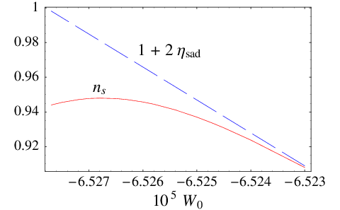
However, quantitatively the models differ by factors. In our example (22) with we choose the same values as in the example discussed in the original racetrack paper. Our values for , , and , at the minimum are of the same order of magnitude, but are not the same. It is therefore very surprising, that despite the quantitative differences in parameter and field values, we also found , irrespective of the exact form of the Kähler potential for the -field. The improved racetrack model [9], which employs two moduli fields , also gives . This therefore seems to be a robust prediction of inflation with racetrack potentials.
 (a)
(a)
 (b)
(b)
In all three versions of the racetrack model the potential during inflation when COBE scales leave the horizon, is of the form
| (24) |
with the slowly rolling inflaton field, and the other fields nearly constant. Indeed in our model are nearly fixed near the saddle, and one can approximate the -dependent functions with constants. In this approximation the kinetic term can be made canonical by a constant rescaling of the field . The only difference with the racetrack models is that the and the kinetic term change after observable inflation, when the “spectator” fields relax to their values at the minimum. It will be interesting to see whether the presence of these spectator fields can affect the inflationary predictions. If, on the other hand, all physics were to be well captured by the potential (24) above, then this would explain the universality of racetrack model predictions for the inflationary observables.
The potential (24) is sufficiently simple that we can explicitly scan the parameter space for saddle points which are flat enough for inflation, at least numerically33 3 Here we restrict ourselves to potentials with saddles at , as has been done in all analyses of the various racetrack models.. To this end we solve for the following conditions:
- 1.
there is a minimum at : (and )
- 2.
the cosmological constant is zero:
- 3.
the saddle at is flat:
- 4.
the potential is scaled to fit the observed power spectrum: .
These four conditions fix all the . The values of and are chosen as in (22). The resulting spectral index depends only on the value of at the saddle; for different values for , but the same (determined by the precision to which condition (3) above is solved) the spectral index is the same. The dependence on is small. This is shown in figure 3b, where is plotted as a function of . For all , guaranteeing enough -folds of inflation, the spectral index .
Figure 3b also shows the corresponding results for our -term uplifted racetrack model. The prediction for the spectral index is practically identical. We can thus conclude that the physics of racetrack is well captured by the simpler potential (24). This explains the universal prediction for the spectral index in all racetrack models.
Although the spectral index only depends on , and not the other parameters, the degree of fine tuning of the potential does depend on those parameters. For example, taking , and as in (22), we find that tuning at the 1% level requires tuning at the level of 44 4 I.e. changing the parameters will give . This agrees with the tuning in the racetrack scenario: changing will change for the parameters (22) and (the first entry of table 1).. Increasing by an arbitrary factor decreases this tuning by about the same factor. The same applies for a scaling of , or a simultaneous scaling of . The degree of fine tuning is most sensitive to , and the larger their difference the smaller the tuning. For example, taking changes the level of fine tuning to . We note however, that in a specific racetrack model, the values of are related, and cannot be adjusted independently. Moreover needs to be sufficiently small to assure .
6 Conclusion
In this paper we have presented a racetrack model embedded in a moduli stabilisation scenario with an uplifting -term. In addition to the volume modulus , a meson field is added to the model to guarantee gauge invariance. The resulting model is completely described by an effective supergravity theory, in contrast to the original racetrack models.
The model is qualitatively similar to the other inflation models based on a racetrack superpotential. For certain parameter choices the volume modulus is stabilised in a Minkowski vacuum with , ensuring the validity of the effective theory. Inflation takes place near a saddle of the potential. During the initial stages of inflation, including the time observable scales leave the horizon, the slowly rolling inflaton field can, to a very good approximation, be identified with . However during the final stages of inflation all fields come into play.
The height of the potential can be scaled to fit the COBE normalisation of the density perturbations. Tuning is needed to make the saddle sufficiently flat for inflation and to get a spectral index that is slightly red shifted. Although the saddle point can be tuned arbitrarily flat, we found an upper bound on the spectral index . This result for the index is the same as in the original racetrack models, and seems to be a robust feature of racetrack inflation. This follows from the approximate equivalence of racetrack inflation to a single field model, obtained by truncation of the full dynamics, in which only is allowed vary.
References
References
- [1] S. Kachru, R. Kallosh, A. Linde, J. M. Maldacena, L. P. McAllister and S. P. Trivedi, Towards inflation in string theory, JCAP 0310 (2003) 013 [hep-th/0308055]
- [2] E. J. Copeland, A. R. Liddle, D. H. Lyth, E. D. Stewart and D. Wands, False vacuum inflation with Einstein gravity, Phys. Rev. D 49 (1994) 6410 [astro-ph/9401011]
- [3] G. R. Dvali and S. H. H. Tye, Brane inflation, Phys. Lett. B 450 (1999) 72 [hep-ph/9812483]
- [4] E. Silverstein and D. Tong, Scalar speed limits and cosmology: Acceleration from D-cceleration, Phys. Rev. D 70 (2004) 103505 [hep-th/0310221]
- [5] M. Alishahiha, E. Silverstein and D. Tong, DBI in the sky, Phys. Rev. D 70 (2004) 123505 [hep-th/0404084]
- [6] P. Binetruy and M. K. Gaillard, Candidates For The Inflaton Field In Superstring Models, Phys. Rev. D 34 (1986) 3069
- [7] T. Banks, M. Berkooz, S. H. Shenker, G. W. Moore and P. J. Steinhardt, Modular Cosmology, Phys. Rev. D 52 (1995) 3548 [hep-th/9503114]
- [8] J. J. Blanco-Pillado et al., Racetrack inflation, JHEP 0411 (2004) 063 [hep-th/0406230]
- [9] J. J. Blanco-Pillado et al., Inflating in a better racetrack, JHEP 0609 (2006) 002 [hep-th/0603129]
- [10] S. Kachru, R. Kallosh, A. Linde and S. P. Trivedi, De Sitter vacua in string theory, Phys. Rev. D 68 (2003) 046005 [hep-th/0301240]
- [11] C. P. Burgess, R. Kallosh and F. Quevedo, de Sitter string vacua from supersymmetric D-terms, JHEP 0310 (2003) 056 [hep-th/0309187]
- [12] A. Achucarro, B. de Carlos, J. A. Casas and L. Doplicher, de Sitter vacua from uplifting D-terms in effective supergravities from realistic strings, JHEP 0606 (2006) 014 [hep-th/0601190]
- [13] E. Dudas and Y. Mambrini, Moduli stabilization with positive vacuum energy, JHEP 0610 (2006) 044 [hep-th/0607077]
- [14]
F. Buccella, J. P. Derendinger, S. Ferrara and C. A. Savoy,
Patterns of Symmetry Breakings in Supersymmetric Gauge
Theories, Phys. Lett. B 115 (1982) 325
R. Gatto and G. Sartori, Consequences Of The Complex Character Of The Internal Symmetry In Supersymmetric Theories, Commun. Math. Phys. 109 (1987) 327 - [15] D. N. Spergel et al. [WMAP Collaboration], Wilkinson Microwave Anisotropy Probe (WMAP) three year results: Implications for cosmology, Astrophys. J. Suppl. 170 (2007) 377 [arXiv:astro-ph/0603449].
- [16] K. Choi, A. Falkowski, H. P. Nilles and M. Olechowski, Soft supersymmetry breaking in KKLT flux compactification, Nucl. Phys. B 718 (2005) 113 [hep-th/0503216]
- [17] P. Brax, A. C. Davis, S. C. Davis, R. Jeannerot and M. Postma, Warping and F-term uplifting, JHEP 0709 (2007) 125 [0707.4583 [hep-th]]
- [18] Z. Lalak, O. J. Eyton-Williams and R. Matyszkiewicz, F-term uplifting via consistent D-terms, JHEP 0705 (2007) 085 [hep-th/0702026]