Sinh-Gordon Boundary TBA and Boundary Liouville Reflection Amplitude
Abstract
The ground state energy of the sinh-Gordon model defined on the strip is studied using the boundary thermodynamic Bethe ansatz equation. Its ultraviolet (small width of the strip) behavior is compared with the one obtained from the boundary Liouville reflection amplitude. The results are in perfect agreement in the allowable range of the parameters and provide convincing support for both approaches. We also describe how the ultraviolet limit of the effective central charge can exceed one in the parameter range when the Liouville zero mode forms a bound state.
PTA/06-19
RIKEN-TH-85
1HAS Theoretical Physics Research Group, H-1117 Budapest
Pázmány s. 1/A, Hungary
2Department of Physics and Research Institute of Physics
and Chemistry, Chonbuk National University, Jeonju 561-756, Korea
3Laboratoire de Physique Théorique et Astroparticules,
UMR-5207 CNRS-UM2, Université Montpellier II, Pl.E.Bataillon,
34095 Montpellier, France and Service de Physique Théorique,
CNRS - URA 2306, C.E.A. - Saclay F-91191, Gif-sur-Yvette, France
1 Introduction
It is often taken for granted that the short distance asymptotic of a two dimensional relativistic field theory is described by a conformal field theory (CFT). This conception leads to the working hypothesis that a massive field theory can be considered as a perturbation of its limiting CFT (CPT) by a relevant operator (or by a combination of relevant operators) [1]. The corresponding (typically dimensional) coupling constant determines the mass scale of the perturbed model. This simple scheme holds for the most studied perturbed rational CFT’s and for certain other models like the sine-Gordon or the imaginary coupled Toda field theories. The CPT approach also provides a systematic description of the corrections to the ultraviolet CFT asymptotics (with certain reservations concerning the non-analyticity in the couplings of the vacuum expectation values, see e.g., [2]). This picture is particularly applicable for finite size effects, like the Casimir energy [3], where CPT is applied literally and is often convergent (see e.g. [4, 5]). There are, however, field theory models of different type, where the short distance asymptotic is considerably more complicated and, up to now, no systematic description in terms of CPT or something similar is known. Conventionally these models can be called the “non-compact” ones, since sigma-models with non-compact target spaces are mostly of this type and reveal the same (or sometimes more severe) peculiarities of which we’re going to discuss now.
The simplest example is the familiar sinh-Gordon model. This model has been studied for a long time and is one of the first discovered integrable theories [6, 7]. The factorized scattering amplitude is one of the simplest possible and the complete set of form-factors of the basic fields is known in a very explicit form [8, 9]. Many other characteristics such as the vacuum energy and even the vacuum expectation values (one point correlation functions) [10] are known exactly (see below for a brief review). In addition, the most general integrable boundary condition has a quite simple form and the corresponding factorized boundary scattering admits a complete description [11, 12]. (This will be recapitulated briefly in section 4).
However, it was recognized quite a while ago [13] that the short distance asymptotic of this apparently simple model is much more involved than the simple CPT scenario pictured above. Even if we do not talk about the short distance behavior of the correlation functions, which is not yet well understood even on a qualitative footing (see e.g., [9] for some preliminary results), the ultraviolet behavior of the Casimir energy behaves in quite a different way from what we’re used to in CPT. The corrections to the formal CFT predictions behave much softer than the usual series in appropriate powers of the scale. It was realized [14] that these leading soft corrections are mostly controlled by the so-called Liouville reflection amplitude (LRA), a quantity of importance in the explicit construction of the Liouville field theory (LFT) [14, 15]. (For an explicit construction based on the conformal bootstrap see [16].) Although there are serious arguments to believe that LFT plays also an important role in the description of the UV asymptotics of other observables, including correlation functions, the finite size settlement is probably the one where our current understanding is the best. The relation between the UV behavior of finite size energy and the reflection amplitudes in related non-rational CFT’s, similar to what was first argued in [14] for the sinh-Gordon case, has been observed in other integrable 2D models of “exponential interaction”, such as SUSY sinh-Gordon [17], affine Toda systems [18] and the generalized sausage model [19, 20].
In the present publication we report a study of a somewhat different settlement of the Casimir problem where, instead of restricting the system to a finite circle with periodic boundary conditions, we put it to a finite interval with integrable boundary conditions at both sides. The ground state energy in this case is measured by means of a modified version of the thermodynamic Bethe ansatz (TBA), the boundary TBA (BTBA) [21]. The UV corrections in this case turn out to be related to the boundary Liouville reflection amplitude (BLRA), the boundary Liouville version of LRA. The system under consideration turns out to be much more rich in physics than the periodic circle one, since the boundary conditions provide enough parameters to reach physically interesting regimes. But before turning to these interesting topics, let us briefly remind the standard periodic Casimir effect of the sinh-Gordon model to establish the convention.
The bulk sinh-Gordon model is defined by the Lagrangian density
| (1) |
Here is a two-dimensional scalar field, a dimensionless parameter and a dimensional coupling constant which determines the scale of the model. In particular the physical mass of the basic (and the only stable) particle of the model is related to as [22]
| (2) |
where is another convenient parameter, often used instead of
| (3) |
The model is integrable and its factorized scattering theory is completely characterized by the scattering amplitude
| (4) |
The knowledge of the scattering theory allows one to apply the TBA to find the finite size ground state energy of the model living on a periodic circle of circumference
| (5) |
The infinite volume bulk vacuum energy is also known exactly [10, 23]
| (6) |
and is the solution to the non-linear integral TBA equation
| (7) |
( stands for the convolution in ). The kernel is related to the ShG scattering amplitude (4) as
| (8) |
In view of Eqs. (2, 4, 6), the ShG model possesses the weak-strong duality, (or ), thus the analysis is restricted to (or ).
It is also convenient to introduce the “effective central charge”
| (9) |
instead of . The most important asymptotic part of the effective central charge at can be described in terms of the “Liouville quantization condition” as
| (10) |
where is the solution of the transcendental equation [14],
| (11) |
is the phase of the LRA
| (12) |
which reads explicitly
| (13) |
Here is the same coupling constant as in Eq. (1) and in the Liouville context is called the bulk cosmological constant. Explicit arguments leading to the relation in Eq. (11) will be given in section 2, for the more complicated case of the “open” finite size effects. We mention here only that LFT can be obtained formally as a kind of “reduction” of the Lagrangian (1): Neglecting one of the exponentials in the interaction term, , we are left with the familiar bulk Liouville Lagrangian
| (14) |
The former is known to define a non-rational CFT with central charge
| (15) |
where is yet another convenient parameter
| (16) |
and is, for historical reasons, called the “Liouville background charge” .
In what follows we are going to apply the same idea of [14] to the system on a finite strip of length with appropriate “right” and “left” boundary conditions (henceforth referred to as “1” and “2”, respectively), and relate the small asymptotic of the ground state energy to the “boundary Liouville reflection amplitudes” in [24]. At the same time, can be alternatively “measured” through the BTBA. General integrable boundary condition in sinh-Gordon model contains two continuous parameters at each edge (see section 4), so that the “open strip” settlement offers, apart from the overall parameter , four parameters to play with. This makes the problem quite interesting and rich in physical phenomena. We will start with some pedagogical reviews on BTBA and BLRA in the first few sections and provide new results in later sections.
The content is organized as follows. In section 2, we describe briefly the boundary Liouville problem and present the explicit expression for the boundary two-point function first given in [24], which coincides with BLRA up to notations. Here the singularity structure and the strong-weak duality of the theory are manifest in Barnes double-gamma and double-sine function [25] whose definitions and useful relations are found in the Appendix. In section 3, semi-classical “mini-superspace” calculation [26] is presented, which gives an independent support to the BLRA and will feed our intuition in later discussion.
We begin section 4 with a brief survey of the factorized boundary scattering in the boundary sinh-Gordon model [11, 12]. Section 5 is devoted to the general formulation of the whole four parameter “open strip” problem. Here we develop the usual “zero mode dynamics” arguments, which relate the UV behavior of to the “boundary Liouville quantization equation” (involving two different BLRAs, and ). In section 6, straightforward form of the related BTBA [21] is presented and its analytic properties are discussed. The standard BTBA equation, however, in a certain region of the parameters needs manipulation of the singular behavior of the boundary fugacity to improve the slow convergence of numerics. It is to be noted in section 7 that BTBA is insensitive to the sign of the boundary scattering parameters, whereas BLRA is not. This mismatch is again due to the singular behavior of the boundary fugacity in BTBA and appears in other BTBA problems [27, 28, 29] as well. BTBA is modified by introducing an additional term, relating to the sign change of the “one-particle” coupling in the boundary state [11]. In section 8, the BTBA equation is solved numerically and is compared to the result of BLRA. Small asymptotic from BTBA with at least one edge “symmetric” (having non-singular fugacity), is found in excellent agreement with the BLRA result when the parameters are away from the singularity domain of BLRA. Inside the singularity domain, BRLA shows that Liouville zero mode is not traveling anymore but trapped to form a bound state, which in turn make the UV limit of the effective central charge to exceed one. BTBA with both edges “asymmetric’ (having singular fugacity) supports perfectly the BLRA result. Section is devoted to the analytic calculation of the boundary condition dependent UV central charge from BTBA and. The result is found to be in agreement with the one coming form BLRA providing another confirmation of the conjectured relation between the UV and IR parameters. Section 10 is the summary and discussion.
2 Boundary Liouville reflection amplitude
Let us consider Liouville field theory (14) on a strip of width , parametrized by the transversal (“space”) coordinate and the “time” along the strip. The complex coordinates are, as usual and . Conformally invariant right and left boundary conditions are described by the action
| (17) |
where, as before, the parameter is related to the LFT central charge (15) with (16). and are called the “right” and “left” “boundary cosmological constants” as the bulk cosmological constant, and are conveniently parametrized in terms of the dimensionless parameters and [24]
| (18) |
Since are real they will be parametrized as follows: When , with real and positive. When , with real. When , there are serious reasons to believe that BLFT is not stable anymore and we exclude this range from the investigations.
Let us denote the space of states of the LFT on the strip. Conformal invariance entails the existence of a (single in this case) set of generators which form the Virasoro algebra
| (19) |
It acts on , splitting into a set of its highest weight representations. The Hamiltonian, the translation generator in , is
| (20) |
The best way to understand the structure of is to take the “zero mode” of the Liouville field
| (21) |
and consider the region in the configuration space where . Both the bulk and boundary interaction terms vanish in this region and we are left with the free massless boson on the strip with free boundary conditions on both boundaries. It is convenient, therefore, to decompose in the oscillator modes
| (22) |
Here
| (23) |
while the oscillators satisfy
| (24) |
The Virasoro generators in this “free field” region are combined as follows
| (25) |
It is easy to argue (see [14]) that the conformal invariance of the boundary theory prescribes the wave function of a primary state of dimension to have the following asymptotic in the region
| (26) |
It is the coefficient near the “reflected wave” what is called the BLRA. Exactly as in the case of “bulk” reflection [14], the boundary reflection amplitude is unitary
| (27) |
with the phase real at real . The standard arguments of real analyticity require the analytic unitarity
| (28) |
In the usual boundary CFT language the primary state (26) is interpreted as the one created by the (juxtaposition if the right and left boundary conditions are different) boundary operator
| (29) |
Hence, under a proper normalization the Liouville boundary reflection amplitude is directly related to the boundary two-point function , introduced and found in [24]
| (30) | ||||
Here and are the standard double-gamma and double-sine functions invented by Barnes [25] (see the Appendix for a brief list of definitions and useful relations).
The BLRA is simply the same quantity with
| (31) |
It is a meromorphic function of and its phase allows the power expansion,
| (32) |
For practical calculations it is convenient to represent the phase (27) in the form
| (33) |
where is the bulk Liouville reflection phase (12), while the -dependent part admits a convenient integral representation
| (34) |
where . It is essentially a Fourier transform and is very convenient for numerical implementation.
The states with real values of the momentum generally constitute the continuous spectrum of “physical” states
| (35) |
All these states are characterized by the energy . There are, however, certain situations when additional “discrete” states appear. This happens if the reflection amplitude has a pole at some with . Then in the asymptotic (26), the incident wave is absent and the state is localized. The pole can appear when at least one of or is negative enough. In the -parametrization the related poles in the BLRA (31) appear at
| (36) |
where stands for the greatest integer less than or equal to and the boundary parameters are limited as
| (37) |
(The right hand side inequality follows from the requirement of the stability of the system ).
For later comparisons let us quote here the semi-classical expression for BLRA (31): in the limit , and while and kept fixed
| (38) |
where .
3 “Mini-superspace” approximation
In this section we provide a semi-classical confirmation of the BLRA (38). Let us consider the semi-classical regime where while and the boundary parameters are kept fixed so that
| (39) |
In the mini-superspace approximation one neglects all the oscillator modes, replacing the Fock space by the vacuum state, and takes into account only the dynamics of the “zero mode” (21). The Hamiltonian (20) is replaced by
| (40) |
The corresponding eigenfunction of momentum solves the second order linear differential equation
| (41) |
This is a degenerate hyper-geometric equation. Appropriate solution is
| (42) |
where and
| (43) |
is the Whittaker function [30]. At
| (44) |
Thus the boundary reflection amplitude in this approximation reads
| (45) |
in complete agreement with the corresponding limit of the exact BLRA (38).
4 Boundary sinh-Gordon scattering
In this section we analyze the sinh-Gordon model with the Lagrangian (1) in the half-space . The boundary theory is specified by the boundary action, which in the most general integrable case has the form [11]
| (46) |
It will be convenient to parametrize the boundary coupling constants following (18) through the (self-dual) parameters and as follows
| (47) |
Integrable boundary conditions are characterized either through integrable boundary interactions or through factorized boundary scatterings. The relevant amplitude of the factorized off-boundary scattering is easily figured out from ref.[11]. It reads as [12]
| (48) |
where the “minimal” amplitude is independent of the boundary parameters
| (49) |
Note that is singular at , which corresponds to the emission of a zero momentum particle by the boundary state in the crossed channel, see [11] for the details.
The second multiplier gives the boundary parameter dependence
| (50) |
Here and are related to the self-dual parameter [24, 31]
| (51) |
Henceforth, we will call the “symmetric” boundary the one with (or ). For the symmetric boundary we have
| (52) |
Let us quote here the expression for the boundary energy as the function of the boundary parameters and
| (53) |
where, as in (6), is the mass of the fundamental particle of the sinh-Gordon scattering theory. At the best knowledge of the authors this expression has never been obtained rigorously. The best way to derive it is to apply the standard relation between the BTBA kernel and the bulk and boundary energy (see [32] or [31] for details). However, strictly speaking this relation is justified only in the case of a standard ultraviolet pattern of perturbed rational CFT. It is the regular perturbative structure of the short distance corrections which allows to require the cancellation of the linear and constant terms [32]. In the case of the sinh-Gordon theory this is certainly not the case. As we mentioned in the introduction, the ultraviolet structure is more complicated and it is not clear for us how to ask for such cancellation against a background of much bigger “soft” corrections. Another way would be to relate the exact one-point function of the boundary operator to [24, 31]. However this is not a derivation, since exactly this relation has been used to figure out the relation (51) between the Lagrangian and parameters of the scattering theory. Although to our conviction there are no doubts about that expression (53) is correct, in the absence of a rigorous derivation the analysis presented below can be considered as its important support.
5 Sinh-Gordon on a strip
Now we are ready to consider the whole problem of the sinh-Gordon model on a finite strip with two different boundary conditions at the right and left boundaries. Let be the width of the strip. Apart from the bulk parameters and , we need four extra boundary parameters to characterize the boundary interaction at the right and left boundaries. They enter the strip action
| (54) |
in the following way
| (55) | ||||
Accordingly we need four parameters in the usual way related to
| (56) |
Scaling properties of the bulk and boundary fields allow to reduce the width of the strip to while rendering the dependence directly to the coupling constants. This is achieved through the rescaling and . The rescaled Lagrangian reads
| (57) | ||||
Notice that the boundary parameters (56) are unchanged under this rescaling.
For our present analysis it is a good idea to single out the “zero mode” (21) of the field and introduce the “oscillator” operators through (22), (23) and (24). The following Hamiltonian corresponds to (57) (compare with (20))
| (58) | ||||
Here the exponentials are thought as normal ordered with respect to the operators , e.g.,
| (59) |
In the present study we are interested in the ground state energy of the strip system. In terms of the Hamiltonian (58) it reduces to finding its lowest energy eigenvector
| (60) |
in the space of states
| (61) |
Of course in general this is a complicated infinite dimensional problem. However, in the narrow strip (ultraviolet) asymptotic , which we mostly consider in the present study, there is always a wide “free region” if , where both the bulk and the boundary interaction terms in (58) can be neglected (see [13] for similar considerations in the “closed” geometry). Here an approximation similar to the mini-superspace one of section 3 is rightful and
| (62) |
where we introduced a ( dependent) “momentum” parameter . This parameter is fixed by the solution of the problem outside the free region, requiring a usual decay of at . In our approximation we neglect and at , reducing the problem to the boundary Liouville one.
| (63) |
Similar analysis of the interaction at results in
| (64) |
Eqs. (63) together with (64) give the boundary version of the “Liouville quantization condition” (BLQC) and for the ground state is chosen as the solution to the transcendental equation
| (65) |
Equations (62) and (65) with the boundary Liouville reflection phases constitute our approximation. In the limit the solution to is small
| (66) |
Therefore the smaller the value of , the better is our approximation. On general footings we expect that the leading correction to Eqs. (62) and (65) are of order (see [33] for analogous consideration about the cylinder case). In view of (66) this means that this correction is exponentially small in and is of the order of .
6 Boundary TBA equation
Formally the BTBA equation gives the strip ground state energy [21]
| (67) |
where ( is the solution to the BTBA equation
| (68) |
Here is ordinary convolution over the real axis of . The strip ground state energy is normalized to compare with the one in (62) obtained using the BLQC.
| (69) |
The quantity is called the boundary fugacity and is given in terms of the boundary scattering amplitude in Eqs. (49) and (50) as:
| (70) |
where is given in terms of the boundary factorized scattering amplitude Eqs. (49, 50)
Explicitly, the fugacity reads
| (71) | |||||
Let us note that is in general singular at , which reflects the one-particle emission at the boundary [11]. However, this singularity vanishes if at least one of the boundaries is chosen, say, , to be symmetric. Then, the double pole in is canceled with the double zero of and the one-particle emission disappears. In this case the numerical analysis of the BTBA equation (68) does not show any slow convergence. Strictly speaking this is the validity range of the original derivation of the BTBA equation (68) in [21] and we are safe to apply it only in this domain. Its extension for the case when both one-particle boundary couplings are non-vanishing requires some care and we devote the next section to this issue.
7 BTBA equation with both edges asymmetric
If both boundaries are asymmetric we face with conceptual and numerical problems. As the infrared analysis in [34] showed the BTBA equation (68) describes properly the ground state energy only for . Even in this case the numerical analysis is also in trouble since even though the convolution integration in (68) is finite, numerical evaluation is very slow in convergence.
To avoid this, one may rewrite the BTBA so that the convolution of the singular part is analytically integrated out. One way is to put
| (72) |
where
| (73) | |||||
| (74) | |||||
Here and is the residue of the fugacity, identified as
| (75) |
This form of the boundary TBA results in the energy of the form
| (76) |
where the one particle contribution is manifested at large distances. For it is in accordance with the boundary analog of the Lüscher type correction [34] and can be further expanded in even number of particle contributions, i.e., powers of for sufficiently large volume.
There are other choices to de-singularize the BTBA. Another useful form [35, 36, 37] is given as
| (77) |
where
The energy in this case has the form
| (78) |
Not only the infrared analysis suggests that the BTBA equation (68) cannot be correct for any choice of the boundary parameters if but this can be seen also from the UV analysis: The strip ground state energy obtained from BTBA Eq. (69) is not sensitive to the sign change of since the boundary fugacity in Eq. (71) is not changed. On the other hand, the energy Eq. (62) from the BLQC is sensitive to the sign change of as we show now. Suppose we change into , then according to the relation (51) turns into and vice versa so that the quantization in Eqs. (65) reads
| (79) |
This change is serious if (see Eqs. (33, 34)). Thus, raises a serious question which one is correct.
This mismatch is also noted in the context of other different BTBA problems [27, 28, 29]. It turns out that the source of trouble is the singular behavior of the fugacity and to cure the trouble one needs to modify the original BTBA in Eq. (68) when .
The correct equation can be obtained by analytical continuation in the one-particle boundary coupling in a model-independent way: To initiate, one notes that the double pole of the fugacity induces a pair of zero singularity satisfying
| (80) |
on the imaginary rapidity axis. This can be easily seen at the infrared (IR) limit. In this case putting the zero positions and noting , one has for Eq. (80)
The double pole structure of the fugacity results in the zeroes at, with a good approximation
| (81) |
which is exponentially close to the pole at the origin.


The convolution integral along the real axis is finite. In order to describe the opposite sign of (or ) case, one analytically continues the BTBA equation by deforming the integration contour and picking up the zero singularity contribution as shown on Fig. 1. If one integrates by part the convolution term turns the zero of the logarithm argument to a pair of pole singularities. Finally one arrives at the compact form of the new BTBA equation,
| (82) |
where is the positive solution of the zero singularity
| (83) |
The modified energy has the form
| (84) |
One may see the implication of this result easily at the IR limit. The dominant energy becomes, with the help of in (81),
| (85) |
which flips the sign of the IR contribution in (76). This result is in agreement with the boundary analog of the Lüscher type correction [34]. Its confirmation in the UV region will be provided by comparing its numerical solution with the one obtained from the BLRA in the next section.
8 Numerical study
In the previous sections we presented two different expressions for the strip ground state energy; one from BLQC Eqs. (62 ,65) and the other from BTBA Eqs. (68, 69) or Eqs. (82, 83, 84). These expressions are given either as a transcendental equation or as a nonlinear integral equation and are not easy to compare using the analytic expression. In this section, we provide the numerical study in a variety of parameter range.
We first note that the BLRA gives the explicit expression of in (34) and in (12, 13). On the other hand, the ground state energy is obtained through the BLQC Eq. (65)
| (86) |
which relates to the scale . Thus, to compare the two different approaches, we are enough to find the relation using the BTBA. This relation is obtained via the effective central charge through Eq. (69), since the corresponding momentum is given as
once we use Eq. (62). Then, the Liouville boundary phase from the BTBA is given as
| (87) |
Thus, the numerical check is to compare (87) with the analytic expression (34). It is noted that the bulk expression in (12, 13) turns out to be in excellent agreement with the TBA result even up to the order of (see some of the results in Ref. [14]).

8.1 Symmetric case
We first restrict ourselves to the case with at least one edge being symmetric, i.e., or since in this parameter range, we can avoid the singular behavior of the boundary fugacity . The simplest case is when both boundaries are symmetric so that the right edge also has or but is not necessarily the same as . Here we can use that (). In this case, Eq. (87) simplifies to
| (88) |
In Fig. 2 the numerical results for are compared with the analytic boundary Liouville expression for the case of two identical boundaries at with purely real values of . Another plot is presented for imaginary values of in Fig. 3.

0.06651092551935 0.41762001693342 0.41762001693341 0.07278412235910 0.45306073688754 0.45306073688672 0.08039322566412 0.49476603900486 0.49476603897984 0.08983119563236 0.54444716822153 0.54444716749005 0.10187859377520 0.60443320709236 0.60443318659429 0.11785948248982 0.67790492787209 0.67790438878486 0.14024177942679 0.76910412419994 0.76909136428327 0.17429836730472 0.88301300229112 0.88276474709427 0.23395539043946 1.02163214862749 1.01846195305733 0.36739025335041 1.15834702793920 1.14485912927470 0.74325569097388 1.19642293140014 1.21070661865468
At smaller than the numerical agreement is impressively good, as it is illustrated in Table 1 for the example of .
The agreement is also quite good up to where the values of are already well bigger than the correlation length and we expect the power corrections in to come into play. This can be explained by the fact that after the contributions of the boundary and bulk vacuum energy are added in Eq. (69), the power corrections to begin with a rather high power of (indeed, they are expected to be at ).
Different boundaries with and , allow to measure the Liouville reflection phase . In Fig. 4 the results are presented for and .

8.2 Discrete mode’s case
As far as one of the edges is symmetric, the two approaches, BTBA and BLRA, are in good agreement. However, as and approach to the critical value , where becomes singular, the agreement fails except at a small region of , which is seen in Fig. 3 when and (in this case the actual critical value is ). In fact, there is a parameter range where exceeds the critical value so that the BLRA has the pole at imaginary value of Eq. (36) and at the same time, Im( and Im( for so that there is no boundary bound state in the IR boundary scattering theory. This range is given by the following conditions satisfied simultaneously:
| (89) |
In this region, the UV limiting value of exceeds 1 as shown in Fig. 5. Then, a question arises: How is in Eq. (69) related to the one Eq. (62) from BLQC?

| BTBA | ||
|---|---|---|
| -39.9 | 1.022497070241340 | -13.125612063335536 |
| -34.9 | 1.022489761509328 | -11.874296674954588 |
| -29.9 | 1.022464134631873 | -10.620393772536636 |
| -24.9 | 1.022373521967475 | -9.359087748545065 |
| -19.9 | 1.022045862147555 | -8.077079274139289 |
| -14.9 | 1.020790366172398 | -6.736968924454419 |
| -12.1 | 1.018739648008074 | -5.923623092706940 |
| -10.1 | 1.015637398421726 | -5.279891692845977 |
| BTBA | ||
|---|---|---|
| -39.9 | 1.027288737814910 | -13.883502224634348 |
| -34.9 | 1.027284375181948 | -12.526342850041335 |
| -29.9 | 1.027267391791812 | -11.167552023824138 |
| -24.9 | 1.027200890055835 | -9.803579618174346 |
| -19.9 | 1.026935938305069 | -8.423633052788508 |
| -14.9 | 1.025827041718239 | -6.995003046786642 |
| -12.1 | 1.023913306574199 | -6.139867067007655 |
| -10.1 | 1.020921463329385 | -5.473674443519166 |
At first sight, this question seems not to make any sense since the parameters simply violate the convergence of . As discussed in section 2, this corresponds to the case when the primary operator is not reflected at the Liouville potential wall but is trapped inside as a bound state, which can be easily given in the semi-classical approximation in section 3. This happens when is sufficiently negative, but not too, so still maintaining the stability of the system. This suggests that the Hilbert space has the discrete spectrum as well as the continuous one (see also [38, 39]). As a consequence, the bound state energy with Hamiltonian Eq. (58) is given as
where is given in (36).
| (90) |
This will give the UV limiting value of the effective central charges greater than 1.
| (91) |
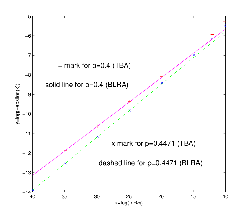
The is given in Table 2 and Table 3 and is plotted in figure 5 corresponding to the parameters , which satisfies the bound in Eq. (89). Eq. (91) predicts when , and when , which agree with the BTBA results. Since BTBA is derived from the saddle point of the partition function it always reproduces the lowest energy state.
We checked this UV limiting value of the effective central charge from BTBA for various ranges of the parameters and found a complete agreement. Interestingly, the leading corrections to the effective central charge are no longer logarithmic in the volume but powerlike. They are not of perturbative origin, however, but are governed by the analytical continuation of the BLQC as we now show. For this we rewrite the BLQC in the exponentiated form
| (92) |
The discrete mode corresponds to the pole singularity of one of the BLRA say . As the volume decreases gets close to the pole at as , so we approximate the BLRA in the neighborhood as
For small enough we determine from (92)
| (93) |
The corresponding central charge can be written as , which gives
| (94) |
In the same spirit we compared the BTBA with the exact BLRA we can calculate from BTBA and compare with the expression (93). The data of from BTBA for various values of at and is given in Table 2 and Table 3 and the log-plot is given in Figure 6. The expected slope is which is for (and for ). The fitted value using the lower 4 points is for (and for ). Small results give more accurate slope and one can see the complete agreement. It proves the correctness of the BLRA not only for real but also for imaginary values of .
8.3 Asymmetric case
Next, we are considering the case when both of the edges are asymmetric. The BLQC is given as a combination of different boundary Liouville phases. Lets us suppose that , thus we have
then if we switch one of the sign of ’s so that , we have
Since individual phases are confirmed already using the case with at least one boundary symmetric, this settlement looks not to provide any new information to the Liouville phase. Nevertheless, this combination is important to check the correctness of the analytically continued BTBA.
The numerical results are in perfect agreement with the exact Liouville amplitude if the improved version of BTBA Eqs. (72, 76) or Eqs. (77, 78) is applied when , and the modified BTBA Eqs. (82, 83, 84) is applied when . This result is plotted in Fig. 7 when , for simplicity. In this case, the phase combination becomes
Other convincing numerical checks are presented in Table (4) and Table (5).

0.077653999816446 -0.039568923372291 -0.039568923376408 0.086205185262923 -0.043897517771010 -0.043897517774418 0.096861805449936 -0.049277259792747 -0.049277259789521 0.110502372967937 -0.056134917955759 -0.056134917808053 0.128563844490344 -0.065154112175326 -0.065154108313167 0.153553843986511 -0.077485060440331 -0.077484967209008 0.190215910849849 -0.095154635137037 -0.095152687636201 0.248446714967505 -0.121766433889740 -0.121735638152979 0.351196987049572 -0.162583158000073 -0.162317800581419 0.556084052286610 -0.216307776233087 -0.216228485970792 1.013529248959518 -0.252173074348906 -0.257965815998832
0.078277417261084 -0.065157660050461 -0.065157660061779 0.086965071942987 -0.072051773672923 -0.072051773682382 0.097806408331036 -0.080511089260293 -0.080511089203979 0.111704015386026 -0.091098590825966 -0.091098589162912 0.130133954494199 -0.104648454630161 -0.104648417456781 0.155666785945641 -0.122400071889728 -0.122399351214232 0.193135842394272 -0.146101177532259 -0.146089809923920 0.252485260446018 -0.177599477043236 -0.177471319390988 0.356217516450171 -0.215816508521331 -0.215038322905223 0.560049812334757 -0.247974299790094 -0.247287310445203 1.014342456385944 -0.256659409495335 -0.262840890495731
9 Calculation of the UV central charge from BTBA
In this section we analyze the UV behavior of the BTBA equation (68). We are able to describe the leading small volume behavior of the central charge analytically using the idea developed in [13]: We expand the Fourier transform of the BTBA kernel
| (95) |
where and write the BTBA equation (68) for the rescaled functions with in the form of an infinite order ordinary differential equation as
| (96) |
We approximate this equation in various rapidity domains in different manners. Since is even we restrict the considerations to the region. Furthermore we are interested in the limit that is we neglect the term, keeping in mind that we have the same contribution from this term in the domain. We distinguish three rapidity regions as follows: , and . If the fugacity term is not relevant but we have to keep all the derivatives of . If we can additionally neglect the term together with higher derivatives of . In this domain, which we call the plateaux domain, is large and positive so we can approximate the BTBA equation as
| (97) |
The corresponding solution is
| (98) |
with two arbitrary parameters, , which can be fixed from the boundary conditions. The corresponding central charge is
| (99) |
As we decrease the volume, , the plateaux region becomes larger and larger and the approximation is better and better. So in this way we describe the leading correction to the central charge.
The boundary condition at is provided by the kinetic term as . In contrast, the boundary condition at the origin is determined by the boundary fugacity. If
| (100) |
then we can demand the boundary condition. This results in
and gives the leading UV behavior of the central charge
which is in accord with the result of BLRA (66).
In the opposite case when , the parameter turns out to be imaginary and we have to fit the parameters of the following function:
| (101) |
Demanding we have . The variable is determined from the boundary condition at the origin, which is provided by the boundary fugacity. Clearly behaves as at the middle of the plateaux region, and we will determine the value of by comparing to the solution around the origin . Here the kinetic term can be neglected (but not the fugacity) and we arrive at the equation
| (102) |
If we additionally suppose that is large negative, which follows from we arrive at the equation
which can be solved by Fourier transformation
where we used the formula
valid for and can be extended for via the relation . We also put and . If in the Fourier transform we have a singular term around the origin as then in its inverse Fourier transform we have a behavior as . So by inspecting the singularity structure around the origin we can extract that
| (103) |
which no longer depends on and increases the central charge. The central charge calculated from yields
| (104) |
which agrees with the result coming form the BLRA (91) when the Liouville zero mode is trapped in the Liouville potential. This gives a convincing analytical support for the UV-IR relation (51) and shows the correctness of both the BLRA and the BTBA.
10 Discussion
We have analyzed the ground-state energy of the sinh-Gordon theory defined on the strip subject to integrable boundary conditions in two complementary ways using BTBA and BLRA.
BTBA, being a nonlinear integral equation, systematically sums up the finite size corrections to the infinite volume ground-state energy by taking into account the information on the semi-infinite boundary scattering theory. As a consequence it is formulated in terms of the boundary reflection factors and is reliable in the IR regime. In the case of the boundary scattering theories corresponding to perturbed rational BCFTs the careful analysis of the UV limit of BTBA allows the determination of the central charge together with the perturbative power-like corrections. We have shown in the paper that, in contrast to this usual behaviour, the UV limit of the boundary sinh-Gordon theory is governed by a non-rational BCFT: the BLFT. The ground-state energy acquires soft (logarithmic) corrections in the volume determined by the BLRA, the most important quantity in the bootstrap solution of the BLFT. This approach is valid in the UV regime and describes the ground-state energy in terms of the parameters of the Lagrangian.
As a first step we solved numerically the BTBA and compared with the predictions coming form the BLRA. In general, we found a convincing evidence of the correctness of both approaches. In particular, we checked the previously conjectured relationship between the IR and UV parameters (51) and confirmed the predictions of BLRA. Then we used the results of BLRA to check the analytically continued BTBA.
The semi-classical picture, provided in the paper, suggested the existence of a discrete part of the Hilbert space, which corresponds to the case when the Liouville zero mode is trapped in the boundary Liouville potential. We confirmed the adequacy of this picture at the quantum level by numerically calculating the effective central charge, which exceeds one in this case. By adopting a method to compute analytically the leading behaviour of the UV central charge we were able to derive its value exactly. This provides another support for both the UV-IR relation and BLRA.
Besides confirming the validity of BLRA, which is a widely used quantity in 2D quantum gravity, we provided evidence for the discrete part of the Hilbert space. It would be interesting to analyze further its consequences.
The way we performed the analytical continuation in the one-particle boundary coupling in BTBA makes possible to apply the result directly to other theories, like boundary Toda theories, where the integrable boundary conditions form a discrete set and there is no room for playing with any continuous parameter. As a consequence, the reflection factors computed from the boundary bootstrap principle in the IR can be compared via the modified BTBA to the parameters of the ATFT valid in the UV. This will help to find the sofar unrevealed correspondence between the two sets of integrable boundary conditions.
In [40] the finite volume description of the sinh-Gordon model originating from an integrable lattice realization was analyzed. It would be nice to perform a similar analysis for the boundary sinh-Gordon theory and explore the analogue of the trapped Liouville mode on the lattice.
Finally, we note that similarly to the analysis of the bulk staircase model [13] its boundary version can be investigated further, along the line of [41], in order to understand better its UV limiting theory.
Acknowledgments. This project was initiated during the focus program of APCTP, 2005 and supported in part by the Joint Research Project under The KOSEF-HAS (F01-2005-000-10282-0)(R&B), by the Center for Quantum Spacetime (CQUeST) of Sogang University with grant number R11-2005-021(R), and by the EGIDE project (Al.Z). One of the authors (Al.Z) thanks the Kawai Theoretical Laboratory at RIKEN, especially H.Kawai and T.Tada, for hospitality and stimulating scientific atmosphere during his visit while this study was finalized. ZB was supported by a Bolyai Scholarship, OTKA K60040 and the EC network “Superstring”.
Note added This work was almost finished last year while two of the authors visited Montpellier and appeared in a final form a month ago. After a communication through the phone with Alyosha on October 15th, we were waiting for his last comment on section 9 which would be done by Thursday (18th). But very sadly and unexpectedly, we are told he passed away on that night. Remembering how excited Alyosha was about the result of this non-compact field theory, we put this draft on the web. We have enjoyed life and discussions with Alyosha.
11 Double gamma and double sine
The double gamma function was introduced by Barnes [25] through the analytic continuation in of the double zeta-series
| (105) |
convergent if (we suppose that ). The analytic continuation can be achieved by the following integral representation
| (106) |
where the contour goes from to encircling the brunch cut of counterclockwise. The double gamma function is defined as
| (107) |
Like ordinary gamma function, is a meromorphic function with no zeros and simple poles located at with a pair of non-negative integers. All these poles are inside the “wedge”
(we imply here that ), which for real shrinks to the negative part of the real axis. Outside the “wedge” it can be represented as the integral which follows directly from (106)
| (108) |
where is the Euler’s constant.
The following dual shift relations are readily derived e.g. from the integral representation
| (109) | ||||
At large outside the wedge the Stirling asymptotic expansion applies
| (110) |
Here are polynomials in defined as
| (111) |
and are usual Bernoulli numbers. One of the effective numerical algorithms is to use several times one of the shift relations (whichever is more convenient) to render the argument to a region where the Stirling formula with a reasonable number of asymptotic terms is effective. For moderate values of the following form also gives quite accurate results
There is also a convenient line integral representation
| (112) |
The diperiodic sine (aka as the Barnes double sine function) is related to as
In the strip it allows the following integral:
| (113) |
Being a Fourier transform this representation is convenient for numerical calculations. Outside the strip of convergence is restored via one of two dual shift relations (which probably inspired the name of the function)
| (114) | ||||
It is a meromorphic function of with poles at with and non-negative integers. The only zeros at are predicted by the “unitarity relation”
| (115) |
which is a direct consequence of (113). The following argument doubling relation is useful to arrive at (30) in the main body of the paper
| (116) |
References
- [1] A. Zamolodchikov, Renormalization group and perturbation theory near fixed points in two-dimensional field theory, Sov. J. Nucl. Phys. 46 (1987) 1090–1987; Higher order integrals of motion in two-dimensional models of the field theory with a broken conformal symmetry, JETP Lett. 46 (1987) 160–164; Integrals of motion in scaling three state potts model field theory, Int. J. Nucl. Phys. A3 (1988) 743–750.
- [2] Al. Zamolodchikov, Two-point correlation function in scaling Lee-Yang model, Nucl. Phys. B348 (1991) 619–641.
- [3] H.B.G. Casimir, On the attraction between two perfectly conducting plates, Proc. Kon. Nederland. Akad. Wetensch. B51 (1948) 793–795.
- [4] Al. Zamolodchikov, Thermodynamic Bethe anzats in scaling three state Potts model and scaling Lee-Yang model, Nucl. Phys. B342 (1990) 695–720.
- [5] F. Constantinescu and R. Flume, The convergence of strongly relevant perturbations of d = 2 conformal field theories, Phys. Lett. B326 (1994) 101–104.
- [6] S.Vergeles and V.Gryanik, Two-dimensional quantum field theories having exact solutions, Sov. J. Nucl. Phys. 23 (1976) 704–709.
- [7] I. Arefyeva and V. Korepin, Scattering in two-dimensional model with Lagrangian , Pisma v ZhETF, 20 (1974) 680.
- [8] A. Koubek and G. Mussardo, On the operator content of the sinh-Gordon model, Phys. Lett. B311 (1993)193–201 [Archive: hep-th/9306044].
- [9] H. Babujian and M. Karowski, Towards the construction of Wightman functions of integrable quantum field theories, Int. J. Mod. Phys. A19S2 (2004) 34–49 [Archive: hep-th/0301088].
- [10] S. Lukyanov and A. Zamolodchikov, Exact expectation values of local fields in quantum sine-Gordon model, Nucl. Phys. B493 (1997) 571-587 [Archive: hep-th/9611238].
- [11] S. Ghoshal and A. B. Zamolodchikov, Boundary S matrix and boundary state in two-dimensional integrable quantum field theory, Int. J. Mod. Phys. A9 (1994) 3841–3886 [Erratum-ibid. A A9, (1994) 4353] [Archive: hep-th/9306002].
- [12] S. Ghoshal, Bound state boundary S matrix of the Sine-Gordon model, Int. J. Mod. Phys. A9 (1994) 4801–4810 [Archive: hep-th/9310188].
- [13] Al. Zamolodchikov, Resonance factorized scattering and roaming trajectories, J. Phys. A: Math. Gen. 39 (2006) 12847–12861.
- [14] A. Zamolodchikov, Al. Zamolodchikov, Conformal bootstrap in Liouville field theory, Nucl. Phys. B477 (1996) 577–605 [Archive: hep-th/9506136]
- [15] H. Dorn and H.-J. Otto, On correlation functions for noncritical strings with but , Phys. Lett. B291 (1992) 39–43 [Archive: hep-th/9206053]; Two and three point functions in Liouville theory, Nucl. Phys. B429 (1994) 375–388 [Archive: hep-th/9403141].
- [16] J. Teschner, Liouville theory revisited, Class.Quant.Grav. 18 (2001) R153-R222 [Archive: hep-th/0104158], A lecture on the Liouville vertex operators, Int.J.Mod.Phys. A19S2 (2004) 436-458 [Archive: hep-th/0303150].
- [17] C. Ahn, C. Kim and C. Rim, Hidden relation between reflection amplitudes and thermodynamic Bethe ansatz, Nucl. Phys. B556 (1999) 505–529 [Archive: hep-th/9903134].
- [18] C. Ahn, V. Fateev, C. Kim, C. Rim and B. Yang, Reflection amplitudes of ADE Toda theories and thermodynamic Bethe ansatz, Nucl. Phys. B565 (2000) 611–628 [Archive: hep-th/9907072]; C. Ahn, P. Baseilhac, V. A. Fateev, C. Kim and C. Rim, Reflection amplitudes in nonsimply laced Toda theories and thermodynamic Bethe ansatz, Phys. Lett. B481 (2000) 114–124 [Archive: hep-th/0002213].
- [19] V. Fateev and Al. Zamolodchikov, The sausage model (Integrable deformations of the 0(3) sigma model), Nucl. Phys. B406 (1993) 521–565.
- [20] V. Fateev, The sigma model (dual) representation for a two-parameter family of integrable quantum field theories, Nucl. Phys. B473 (1996) 509–538.
- [21] A. LeClair, G. Mussardo, H. Saleur and S. Skorik, Boundary energy and boundary states in integrable quantum field theories, Nucl. Phys. B453 (1995) 581–618 [Archive: hep-th/9503227].
- [22] Al. Zamolodchikov, Mass scale in sin-Gordon and its reductions, Int. J. Mod. Phys. A10 (1995) 1125–1150.
- [23] C. Destri and H. deVega, New exact results in affine Toda field theories: Free energy and wave function renormalizations, Nucl. Phys. B358 (1991) 251–294.
- [24] V. Fateev, A. Zamolodchikov and Al. Zamolodchikov, Boundary Liouville Field Theory I: Boundary State and Boundary Two-point Function, LPM-00-05 (2000) [Archive: hep-th/0001012].
- [25] E.W.Barnes, The genesis of the double gamma function, Proc. London. Math. Soc. 31 (1899) 358; The theory of the double gamma function, Phil. Trans. Roy. Soc. A196 (1901) 265.
- [26] C. Ahn, C. Kim, C. Rim, Reflection amplitudes of boundary Toda theories and thermodynamic Bethe ansatz, Nucl. Phys. B628 (2002) 486-504 [Archive: hep-th/0110218].
- [27] P. Dorey, I. Runkel, R. Tateo and G. M. T. Watts, -function flow in perturbed boundary conformal field theories, Nucl. Phys. B578 (2000) 85–122 [Archive: hep-th/9909216].
- [28] J. S. Caux, H. Saleur and F. Siano, The Josephson current in Luttinger liquid superconductor junctions, Phys. Rev. Lett. 88 (2002) 106402 [Archive: cond-mat/0109103]; J. S. Caux, H. Saleur and F. Siano, The Two boundary sine-Gordon model, Nucl. Phys. B672 (2003) 411–461 [Archive: cond-mat/0306328].
- [29] T.-J. Lee and C. Rim, Thermodynamic Bethe ansatz for boundary sine-Gordon model, Nucl. Phys. B672 (2003) 487–509 [Archive: hep-th/0301075]
- [30] E. T. Whittaker, G. N. Watson, A course of modern analysis, 4th Edition, Cambridge University Press, Cambridge, UK, 1927.
- [31] Z. Bajnok, L. Palla, G. Takacs, Finite size effects in boundary sine-Gordon theory, Nucl. Phys. B622 (2002) 565–592 [Archive: hep-th/0108157].
- [32] P. Dorey, A. Pocklington, R. Tateo and G. Watts, TBA and TCSA with boundaries and excited states, Nucl. Phys. B525 (1998) 641–663 [Archive:hep-th/9712197].
- [33] Al. Zamolodchikov, On the thermodynamic Bethe Ansatz equation in Sinh-Gordon model, J. Phys. A: Math. Gen. 39 (2006) 12863–12887 [Archive: hep-th/0005181].
- [34] Z. Bajnok, L. Palla, G. Takacs, Finite size effects in quantum field theories with boundary from scattering data, Nucl. Phys. B716 (2005) 519–542 [Archive: hep-th/0412192].
- [35] A. Klümper and P. Pearce, Analytical calculations of scaling dimensions: Tricritical Hard square and critrical hard hexagons, J. Stat. Phys. 64 (1991) 13; Conformal weights of RSOS lattice models and their fusion hierarchies, J. Phys. A 183 (1992) 304.
- [36] V. Bazhanov, S. Lukyanov, A. Zamolodchikov, Integrable quantum field theories in finite volume: Excited state energies, Nucl. Phys. B489 (1997) 487–531. [Archive: hep-th/9607099].
- [37] P. Dorey, A. Pocklington, R. Tateo, G. Watts, TBA and TCSA with boundaries and excited states, Nucl. Phys. B525 (1998) 641–663 [Archive: hep-th/9712197].
- [38] J. Teschner, Remarks on Liouville theory with boundary, [Archive: hep-th/0009138].
- [39] J. Teschner, On boundary perturbations in Liouville theory and brane dynamics in noncritical string theories, JHEP 0404 (2004) 023 [Archive: hep-th/0308140].
- [40] J. Teschner, On the spectrum of the Sinh-Gordon model in finite volume [Archive: hep-th/0702214].
- [41] F. Lesage, H. Saleur, P. Simonetti, Boundary flows in minimal models, Phys.Lett. B427 (1998) 85-92 [arXiv:hep-th/9802061].