The Mott metal-insulator transition in the 1D Hubbard model in an external magnetic field
Abstract
We study the low energy behavior of the one dimensional Hubbard model across the Mott metal-insulator phase transition in an external magnetic field. In particular we calculate elements of the dressed charge matrix at the critical point of the Mott transition for arbitrary Hubbard repulsion and magnetization numerically and, in certain limiting cases, analytically. These results are combined with a non-perturbative effective field theory approach to reveal how the breaking of time reversal symmetry influences the Mott transition.
I introduction
Exact solutions play an invaluable role in our understanding of the behavior of electron systems in one dimension, especially for effective field theory approaches in regimes when strong coupling develops. Here effective theories have to be assisted with a non-perturbative, unbiased analysis. Strong coupling regimes can develop when the initial interactions between electrons are strong, but also in certain situations when the bare couplings are arbitrarily weak. One well known example of the latter case is provided by the so called commensurate-incommensurate phase transition JN; PT, in which a single bosonic mode is involved. By comparing with a free fermions picture the universal physics at long wavelengths across the transition was established JN. A physical system realizing such transition is e.g. the repulsive Hubbard model at half filling, where Mott metal-insulator transition takes place upon variation of the chemical potential in the absence of an external magnetic field. In this case the charge mode undergoes a commensurate-incommensurate phase transition, while the spin sector is decoupled.
In the absence of special symmetries such as time reversal symmetry, however, there is no reason for the decoupling of spin and charge modes. This is well known for the Hubbard model away of half filling in finite magnetic field Frahm. At half-filling, on the other hand, spin and charge modes are strictly decoupled even in an external magnetic field and the low energy sector is equivalent to the Heisenberg antiferromagnet. Here one might be led to think that the admixture between spin and charge modes will die out gradually approaching the half filling.
If this expection would be correct, the Mott metal-insulator transition in the presence of an external magnetic field would look pretty similar to that at zero field: all relevant changes affect only the charge sector, while the spin sector remains practically undisturbed. Thus the phase transition would fall in the the single mode commensurate-incommensurate universality class even in the presence of magnetic field. In the following we will show that the above expectation is misleading. Any small coupling between the spin and charge modes increases under the renormalization and qualitatively influences the critical properties of the system.
II The model
Our starting microscopic model is the Hubbard Hamiltonian of one dimensional lattice electrons:
| (1) | |||||
Here is the number operator of electrons with spin at the -th site, is the local coupling constant, is the chemical potential (half filling corresponds to ), and is an external magnetic field.
The asymptotics of the correlation functions of Hubbard model in the presence of two gapless modes have been computed using a conjecture for a multivelocity ’conformal’ field theory IzKR89 by finite size scaling analysis of the low lying energies of (1) from the Bethe ansatz FrKo90; Frahm. Alternatively, the exact finite size spectrum can be used to determine the parameters of a multi-component Luttinger liquid theory in a non-perturbative way. This way one obtains an explicit expression for the correct low energy effective field theory for the Hubbard model in the sector corresponding to the given filling and magnetic field Penc. In both approaches, the crucial quantity governing the low energy behavior is the dressed charge matrix, being the number of gapless modes in the theory.
We will first try to follow the second approach and work out the effective field theory to better understand non-perturbative effects produced by the magnetic field across Mott metal-insulator transition. Then we will compute elements of dressed charge matrix from the Bethe ansatz, numerically for generic Hubbard coupling and magnetic fields, and in certain limits analytically. Finally we will study response functions and correlation functions and discuss the effects of the magnetic field on the Mott metal insulator transition.
III effective field theory
III.1 Weak-coupling Bosonization
First we recapitulate on the effective field theory of the repulsive Hubbard model at half filling where umklapp processes open a charge gap and the low energy sector of the Hubbard model becomes equivalent to that of the Heisenberg antiferromagnetic chain. When the chemical potential is smaller than the gap in the single particle excitation spectrum (charge gap) the effective Hamiltonian takes the following form Gogolin:
| (2) | |||||
and the only quantities that determine asymptotics of the algebraically decaying correlation functions are spin wave velocity and Luttinger liquid parameter of the spin mode. Clearly, spin and charge modes are perfectly separated in (2). However, away of half filling and for nonzero magnetic field spin and charge degrees of freedom do not separate any more. The reason of the admixture between spin and charge degrees of freedom can be easily traced back to the case of noninteracting electrons. For non-zero magnetization, , the anisotropy of the Fermi velocities (away of half filling) leads to a coupling of spin and charge excitationsPenc; Giamarchi; Kollath. For this coupling is:
| (3) |
For all filling (except of half filling) there is a quadratic coupling between spin and charge modes with an amplitude proportional to the velocity anisotropy at . The modification of this admixture for finite is encoded in the dressed charge matrix. To take fully into account this spin-charge coupling one has to work with the renormalized theory with the initial free value of the coupling amplitude .
III.2 Non-Perturbative Effective Theory
The effective field theory of the repulsive Hubbard model in a magnetic field can be constructed in a non-perturbative way by matching the critical exponents of the multicomponent Luttinger liquid with those of the Hubbard model Penc in the situation where there are two gapless modes. Here, we will carry out this comparison in the limit of the zero doping. In the presence of two gapless modes the following asymptotic expression follows for the primary fields from the hypothesis of multivelocity conformal theories IzKR89:
| (4) |
where the anomalous exponents are defined in terms of the dressed charge matrix as FrKo90:
| (5) | |||||
| (6) |
At the dressed charge matrix takes the form:
| (7) |
with the familiar Luttinger liquid parameters of charge/spin sectors. On the other hand we have , , Woyn89. Therefore, at zero magnetic field one finds and , i.e. the anomalous dimensions of spin and charge fields depend only on spin and charge quantum numbers respectively. This is the essence of spin-charge separation Woyn89; FrKo90. For finite magnetic field, , and below half–filling, , however, this is no longer the case. Here the fields that diagonalize the quadratic Hamiltonian (Luttinger liquid fixed point) are not spin and charge modes, but rather their linear combinations denoted by Penc; Cabra:
| (8) |
Again, the quantity that connects those fields with microscopic physical spin and charge fields is the dressed charge matrix :
| (9) |
and
| (10) |
Note that decoupling of the spin and charge degrees of freedom in the effective Hamiltonian (8) requires and , i.e. and 11 1 The other possibility for decoupling, i.e. and , amounts to a simple relabeling of the gapless modes. In the Hubbard model where charge and spin modes are related to observable quantum numbers the corresponding condition cannot be realized.. As we shall see below the first condition holds for general values of and at half-filling while the second is violated for non-zero magnetic field.
The form (8) of the Hamiltonian is very useful for comparison with the one obtained by ordinary weak- coupling bosonization procedure. In particular at zero magnetization where spin and charge fields are decoupled we can directly read off Luttinger liquid parameters. Indeed, using the explicit expression of dressed charge matrix for zero magnetization in the limit of half filling (see matrix (24) below), the effective theory takes the following form:
| (11) |
implying that the fixed point values for Luttinger liquid parameters are , . Note however, that this theory is valid only at extremely low energies, because the charge wave velocity approaching Mott phase (see Eq. (29)).
Once the elements of dressed charge matrix are determined, susceptibilities as well as correlation functions can be calculated from the above effective theory. In the following we will study the elements of dressed charge matrix at the Mott metal-insulator transition point in the presence of magnetic field by Bethe ansatz method.
IV Dressed charge matrix at half filling
Within the Bethe ansatz approach the dressed charge matrix is a quantity which determines the finite size spectrum and thereby the various susceptibilities for the model. For the Hubbard model it is given as:
| (13) | ||||
Here and , . In the Bethe ansatz approach the boundaries and have to be determined as functions of the filling and magnetization. At half filling one has while is fixed by the condition for the dressed energy of the magnetic excitations (the chemical potential in the Mott phase is ):
| (14) |
Using the integral equations (13) simplify:
| (15) | ||||
With this the dressed charge matrix reads at half filling:
| (16) |
and the remaining entries are determined as 22 2 Alternatively, one can write with , see Ref. [Woynarovich91]. :
| (17) | ||||
For general Hubbard coupling and magnetic field, the integral equations (14) and (15) for and have to be solved numerically to obtain the dressed charge matrix (16) as a function of the magnetic field or the magnetization. In the weak and strong coupling limits, however, one can obtain asymptotic expressions.
For we have the relations , for any electron filling and magnetization Frahm. Therefore we find for strong coupling:
| (18) |
In the weak coupling regime we analyze the integral equations for half filling (14) and (15) for sufficiently small magnetic fields: in this case the boundary of the remaining integration is large. Rewriting eqs. (15) as:
| (19) | ||||
we can apply Wiener-Hopf techniques to compute in the relevant region where the second integral in the first equation of (19) can be treated as a perturbation. To leading order one obtains:
| (20) | ||||
Starting with (20) higher order corrections to can be computed in an iterative scheme YaYa66; Woynarovich91; HubbBook giving the diagonal element of the dressed charge matrix:
| (21) |
Rewriting the expression for in a similar way we obtain:
| (22) | ||||
Finally, has to be expressed in terms of the magnetic field or the magnetization. Applying the Wiener-Hopf technique to Eq. (14) the condition gives:
| (23) |
where HubbBook. In particular, we have for zero magnetic field independent of . As a consequence the dressed charge matrix at half filling for any becomes:
| (24) |
which is the strong coupling limit of the expression obtained in the invariant case below half filling FrKo90. For small fields the leading field-dependence of the dressed charge matrix is the linear (up to logarithmic corrections):
| (25) |
Finally, with the known small field behavior of the magnetization and the spinon velocity HubbBook, this expression can be written as a function of the magnetization :
| (26) |
For the crossover between this exponentially suppressed dependence on 33 3 One can check that the result (26) is consistent with a zero magnetization limit of: , obtained after particle-hole transform from the attractive Hubbard model Woynarovich91. to the one for the strong coupling (18) the Bethe integral equations (14) and (15) have to be solved numerically. The result is shown in Figure 1.
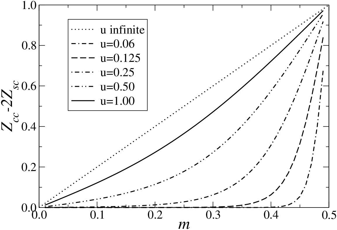
V Susceptibilities and Correlation Functions
Let us now summarize our results for the elements of the dressed charge matrix for general magnetization when doping . As we worked out explicitly in this limit:
(i) : this equation simply reflects the fact that holons are extremely dilute in limit and therefore they do not interact directly with each other.
(ii) : this holds because this element of dressed charge is a smooth function of density and magnetization, which is well defined at half filling and any magnetization. Due to the spin-charge separation it vanishes at half filling.
(iii) depends on magnetization and . In the limit of infinite it approaches the Luttinger liquid parameter of the Heisenberg chain at the same magnetization. For weak coupling we have:
| (27) |
where is the Fermi velocity of the noninteracting electrons.
(iv) The last element that we worked out was . In two limits, namely and analytic expressions were obtained. The most important result is that, generically, in the limit , thus the effective theory does not get completely decoupled in spin and charge parts. This has important consequences on response functions and correlation functions. It is straightforward to study susceptibilities from our effective theory Vekua, and indeed one can see that even at the Mott metal-insulator transition point the exact expressions for the Hubbard model are recovered:
| (28) |
(these and similar expressions for the spin susceptibilities are given in Ref. [HubbBook]). Note that the charge susceptibility remains finite across the Mott transition when the magnetization is kept constant.
On the other hand when the magnetization is not kept fixed, then the charge susceptibility diverges across the Mott metal-insulator transition, and we can estimate how it diverges with the doping. For this we see from Eq. (28) that it is sufficient to calculate the charge velocity as a function of doping. At half filling in the vicinity of the holon band minimum there is a relativistic dispersion (Eq. (7.24) from Ref. [HubbBook]): (corresponding to expansion of the holon band up to second order in momentum) where is the holon velocity at half filling and is a single particle gap. Therefore, below half filling the charge velocity can be obtained asGiamarchi:
| (29) |
In particular for we have and it follows .
Once the elements of dressed charge matrix are determined one can easily obtain correlation functions of physical operators FrKo90; Frahm; Penc; Cabra. We will discuss below only those correlators, which decay algebraically on both sides of phase transition. For the Hubbard model those correlators involve only spin operators EsFr99. The most slowly decaying one in the Mott insulator phase is the in plane spin-spin correlation function. In the metallic phase, i.e. the phase with two gapless modes, the leading correlator is, depending on the strength of , either single field (for small values of ) or again in-plain spin correlator (for large values of ). The equal time correlation function of in plane spin operator reads:
| (30) |
while in the insulating phase it was given by:
| (31) |
Here, we can read off the jump in the critical exponent across the Mott metal-insulator transition as:
| (32) |
Note, that although there is no spin-charge separation the same universal jump of in critical exponent as in the zero-field case is recovered.
VI Conclusions
The presence of a magnetic field breaks time reversal invariance and thereby prevents the separation of spin and charge degrees of freedom in the 1D Hubbard model away from half-filling. In this paper we have studied the effect of the resulting admixture of the gapless modes on the nature of the Mott metal-insulator transition. We have addressed this problem by studying the long wave-length properties of 1D Hubbard model across the transition in an external magnetic field. Using Bethe ansatz techniques we calculated numerically elements of dressed charge matrix for generic cases. In addition exact analytic expressions were obtained in the limiting cases for the same quantity. We also constructed a non-perturbative effective field theory where the drastic effects produced by the time reversal symmetry breaking across the Mott phase transition become manifest: while the susceptibility related to the charge mode which becomes gapped at the transition diverges at half filling for fixed magnetic field (just as in the time reversal invariant case and as known for the free fermion picture JN for the commensurate-incommensurate transition) it remains finite due to the absence of spin charge separation when the magnetization is kept constant. The reason for the behavior in the latter case is that there is always an admixture to the effective field of the magnetic mode which remains gapless across the transition.
VII Acknowledgments
TV acknowledges discussions with Gora Shlyapnikov who motivated his interest in the problem. The work was started while TV’s visit to the University of Hanover supported by the Deutsche Forschungsgemeinschaft. TV also acknowledges GNSF grant No. N . LPTMS is a mixed research unit No. 8626 of CNRS and Université Paris Sud.
References
- (1) G. I. Japaridze and A. A. Nersesyan, Phys. Lett, 85 A, 23 (1981); J. Low Temp. Phys. 47, 91 (1983).
- (2) V. L. Pokrovsky and A. L. Talapov, Phys. Rev. Lett. 42, 65 (1979).
- (3) H. Frahm and V. E. Korepin, Phys. Rev. B 43, 5653 (1991).
- (4) A. G. Izergin, V. E. Korepin, and N. Yu. Reshetikhin, J. Phys. A22, 2615 (1989).
- (5) H. Frahm and V. E. Korepin, Phys. Rev. B 42, 10553 (1990).
- (6) K. Penc and J. Sólyom, Phys. Rev. B 47, 6273, (1992).
- (7) T. Giamarchi, Quantum Physics in One Dimension (Oxford University Press, Oxford, 2004).
- (8) C. Kollath and U. Schollwöck, New J. Phys. 8, 220 (2006).
- (9) A. O. Gogolin, A. A. Nersesyan and A. M. Tsvelik: Bosonization and Strongly Correlated Systems, Cambridge University Press (1999).
- (10) F. Woynarovich, J. Phys. A22, 4243 (1989).
- (11) D. C. Cabra, et al. Phys. Lett. A 268, 418 (2000); Phys. Rev B 63, 094406 (2001).
- (12) F. H. L. Essler, H. Frahm, F. Göhmann, A. Klümper, and V. E. Korepin: The One-Dimensional Hubbard Model, Cambridge University Press (2005).
- (13) F. Woynarovich, Phys. Rev. B 43, 11448 (1990); F. Woynarovich and K. Penc, Z. Phys. B 85, 269 (1991).
- (14) C. N. Yang and C. P. Yang, Phys. Rev. 150, 327 (1966).
- (15) Details will be published elsewhere.
- (16) F. H. L. Essler and H. Frahm, Phys. Rev. B 60, 8540 (1999).