Odd Khovanov homologyThanks: PSO was supported by NSF grant number DMS-0505811 and FRG-0244663Thanks: JR was supported by NSF grant number DMS-0603940 and a Sloan FellowshipThanks: ZSz was supported by NSF grant number DMS-0704053 and FRG-0244663
Abstract.
We describe an invariant of links in which is closely related to Khovanov’s Jones polynomial homology. Our construction replaces the symmetric algebra appearing in Khovanov’s definition with an exterior algebra. The two invariants have the same reduction modulo , but differ over . There is a reduced version which is a link invariant whose graded Euler characteristic is the normalized Jones polynomial.
1. Introduction
In his influential paper, Khovanov [3] describes a link invariant which associates to a link a bigraded Abelian group whose graded Euler characteristic is the Jones polynomial. His invariant is obtained from a TQFT which associates to a collection of embedded, planar circles the symmetric algebra of the vector space generated by the circles. Our goal here is to describe a modified version of Khovanov homology, which associates to a collection of embedded, planar circles the exterior algebra of the vector space generated by the circles.
We explain this invariant. The constructions described here are clearly quite closely related to Khovanov’s. Indeed, the mod two reductions of the two theories coincide (cf. Proposition 1.6 below).
1.1. A projective TQFT
Consider the category of compact one-manifolds and compact, orientable cobordisms between them. The starting point for the construction of the odd Khovanov homology is a “projective functor” from to the category of graded –modules. This functor is “projective” in the sense that the map assigned to a morphism is well-defined only up to an overall sign.
An object is a disjoint union of circles. Given such an , we let denote the free abelian group generated by its components, and define . Morphisms in are generated by four types of elementary morphism: zero-handle additions (or births), one-handle additions where the feet of the one handle lie on two different components (merges), one-handle additions where the feet lie on the same component (splits), and two-handle additions (deaths). We will be most interested in the morphisms corresponding to one-handle additions.
Suppose that is a merge cobordism which joins the circles and in . Then there is a natural identification , and we define
to be the map induced by the projection .
Next, suppose that is a split cobordism in which a single circle in divides to form two circles and in . Then the natural identification induces an identification
The second isomorphism is well-defined only up to sign. We define to be the composition
This map sends to .
For completeness, we record the maps induced by the birth and death cobordisms as well. A birth cobordism induces an inclusion , and is the induced map. In a death cobordism , there is a distinguished component in which is capped off by the two-handle; the map is given by contraction with the dual of .
The reader can easily verify that up to sign, these maps satisfy all the identities associated with a TQFT. We could eliminate the sign ambiguity by tensoring with ; the resulting TQFT can be identified with the reduction of the TQFT used by Khovanov in [3].

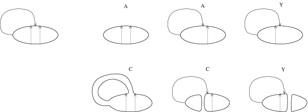
Another approach is to try to deal with the sign ambiguity by decorating our cobordisms. Suppose we have a cobordism with a fixed decomposition into one-handles. Such a cobordism is specified by an -tuple of embedded zero-spheres . These can be represented diagrammatically by joining the two points of by an arc representing the core of the one-handle and fixing an (arbitrary) orientation on it, as shown in Figure 1. If the cobordism associated to the handle addition is a split, we fix the sign of by requiring that it take to , where the arrow points from to .
Given two one-handles , the induced maps commute up to sign:
| (1) |
When the composite map is nontrivial, the sign of can be determined from the combinatorics of how the two arcs and interact with each other, as illustrated in Figure 2. When , we call the pair of Type ; when , we call the pair of Type . There are two remaining cases where the double-composites are trivial. We label these cases by and , as shown in Figure 2.


1.2. The hypercube of resolutions
Given a link projection, we fix an orientation on it by drawing an arrow at each crossing, as illustrated in Figure 3. If is an oriented link diagram of this form, we can define its associated hypercube of oriented resolutions. Specifically, each crossing in the projection has two resolutions and . (These are the resolution conventions of [3]; they are opposite to those from [10].) The crossing can be thought of as giving a cobordism from to consisting of a single one-handle, as illustrated in Figure 3. Let denote the set of crossings of the diagram . Then for each map , we have an associated embedded one-manifold in the plane, which replaces a given crossing by its oriented resolution of type .
Given two vertices in the hypercube, we say that there is an oriented edge from to if there is some with the property that
We let and denote the set of edges and vertices, respectively. Each vertex corresponds to an object in , and each edge in corresponds to a morphism. Given from to , we let denote the corresponding morphism from to .
Two-dimensional faces, or squares, in the hypercube of oriented resolutions correspond to pairs of resolutions for which there are exactly two with
| if |
Each square face may be classified as one of types , , , or , according to the classification scheme in Figure 2.
Definition 1.1.
An edge assignment for a diagram is a map . Given an edge assignment , we say that a square face is even or odd, depending on whether it contains an even or odd number of edges with . A type edge assignment is an edge assignment with the property that all faces of type and are even and all faces of type and are odd. Similarly, a type edge assignment is an edge assignment for which faces of type and are even and faces of type and are odd.
The following lemma will be established in Section 2.
Lemma 1.2.
Any diagram has an edge assignment of type , and one of type .
1.3. The chain complex
Consider the vector space
Given a type or a type edge assignment , we can define an endomorphism of by the formula
for .
We claim that . Indeed, this relation is satisfied provided
whenever we have four edges bounding a square (so that and are the two paths from the initial point to the final point). For a square of type or , this holds by Equation (1), while for squares of type or , the relation holds since
Thus the pair defines a chain complex.
can be equipped with a bigrading , following [3]. Specifically, we endow the exterior algebra with the -grading for which has -grading equal to . Similarly, we define the initial homological grading on so that is supported in grading . The -grading on is then given by , where here denotes the number of negative crossings in the diagram, and the homological grading . We write
where corresponds to the homological grading and the -grading. Since the differential preserves -grading and drops -grading by one, the two gradings descend to homology, and we can write
Theorem 1.3.
Let be a link. Fix an oriented projection of and an edge assignment of type or . The bigraded homology groups of are independent of the choice of and .
We call the above bigraded homology groups the odd Khovanov homology of the link , , to distinguish it from ordinary Khovanov homology (where the variables are “even”). We collect here some properties of which follow quickly from its construction; proofs will be supplied in Section 4.
Recall that the unnormalized Jones polynomial is characterized by the properties that:
where for , we write if for some .
Proposition 1.4.
categorifies the unnormalized Jones polynomial, in the sense that
Exactly as in Khovanov’s original construction, the skein relation characterizing the Jones polynomial is replaced by a skein exact sequence, cf. [3]:
Proposition 1.5.
There is a long sequence
The maps , , and are all homogenous with respect to the bigrading; for a precise statement of the grading shifts, see e.g. [9], [11].
Proposition 1.6.
The mod two reduction of agrees with the mod two reduction of Khovanov’s homology ; i.e.
Despite their formal similarities, and are actually very different groups. The first indication of this fact is given by
Proposition 1.7.
There is a bigraded Abelian group with the property that
We call the reduced odd Khovanov homology. The bigraded group categorifies the ordinary Jones polynomial , which is defined by the relation It analogous to the reduced Khovanov homology defined in [4] which also categorifies the ordinary Jones polynomial, but there are some differences. In the definition of the ordinary reduced Khovanov homology, one fixes a component of ; different choices of component can lead to different answers (which can be seen, for example, by considering the disjoint union of the trefoil and an unknot). By contrast, is a link invariant. Moreover, the relation between and is simpler than the relation between and .
For small knots , the groups and are isomorphic. Indeed, we have
Proposition 1.8.
If is a non-split alternating link, then .
However, there are many nonalternating knots for which the two groups are not isomorphic.
In [10], it is shown that there is a spectral sequence whose term is Khovanov homology of a link , with coefficients taken in , and which converges to the Heegaard Floer homology of the branched double-cover of . Our motivation for finding odd Khovanov homology came from our attempts to lift this to a result over ; and consequently, it is natural to make the following:
Conjecture 1.9.
Let be a link. There is a spectral sequence whose term is the reduced odd Khovanov homology of and whose term is the Heegaard Floer homology of the branched double-cover of (with coefficients in ).
A similar result should hold, with a suitable construction from Seiberg-Witten monopole Floer homology [7] replacing the Heegaard Floer homology of the branched double-cover.
This paper is organized as follows. In Section 2 we construct the edge assignments needed to construct the chain complex (Lemmas 1.2), and show that the isomorphism class of the complex is independent of the choice of sign assignment and the orientations. In Section 3, we show that odd Khovanov homology is independent of the link projection. The arguments here follow closely the invariance proof of Khovanov’s theory (see [3], see also [1], [5], [6]). In Section 4, we establish the basic properties of this construction enumerated above. Finally, in Section 5, we exhibit some calculations of these groups.
We wish to thank Mikhail Khovanov, Tomasz Mrowka, and Paul Seidel for their encouragement during the preparation of this manuscript.
2. Existence and uniqueness of edge assignments
Our first goal in this section is to prove Lemma 1.2, which allows us to construct the chain complex for odd Khovanov homology. We then make some preliminary steps towards the proof of Theorem 1.3 by showing that the isomorphism type of the complex does not depend on or on the choice of orientation at the crossings.
Lemma 1.2 will follow quickly from the following lemma about cubes in the hypercube of oriented resolutions; but before stating this lemma, we note that a cube in the hypercube of resolutions is determined by a pair of resolutions
with the property that there are three crossings such that
Lemma 2.1.
Each cube in the hypercube of resolutions contains an even number of squares of type and . Similarly, each cube contains an even number of squares of type and .
Proof.
This is a case-by-case analysis according to the different possible combinatorial types of cubes in the hypercube of resolutions. Specifically, a cube corresponds to eight resolutions, which are given a partial ordering, with a unique minimal element. The cube is determined by this minimal element () and the three oriented arcs connecting various components (corresponding to three crossings in the original projection). We disregard all the unknotted circles which do not meet these three arcs. This leaves us between one and four circles, which are connected by the oriented arcs (in the plane). We enumerate the possible connected diagrams in Figure 4.

Let , , , and denote the number of squares of types , , and respectively in each cube. We claim that both and are even. This, too, is an easy verification. Note that the six squares in each cube are realized by choosing one of the three arcs, and either dropping it, or performing surgery along it. For example, in Figure 5, we have pictured the possibilities for the second type of cube appearing in Figure 4, with one of the eight different possible choices of orientations. We see that there are two squares of type , two of type , and two of type . The number of squares of types , , , and in the other cases is indicated in figure 4. We leave it to the reader to verify that in all cases, and are even.
If the diagram is disconnected, it has a component with only one arc. We orient the cube so that the four edges corresponding to this arc are vertical; then the top and bottom faces are of the same type. If the vertical edges correspond to merges, all four vertical faces are of type . If they are splits, each merge in the top face corresponds to a vertical face of type , and each split corresponds to a vertical face of type . The number of merges and splits in the top face are both even, so the claim holds in this case as well.
∎
Proof of Lemma 1.2.
Let be the multiplicative group with elements . We consider the hypercube of oriented resolutions as a simplicial complex. We can define on it a -cochain which associates to each face of type or the element , and to each face of type or the number . Lemma 2.1 shows that is a cocycle. Since the cube is contractible, must be a coboundary. Concretely, this means that there is some function with the property that where are the four edges of the square . This is the required edge assignment of type . The same remarks hold for constructing an edge assignment of type . ∎
Lemma 2.2.
If and are two edge assignments of the same type ( or ), then the chain complex is isomorphic to .
Proof.
Suppose that and are two edge assignments of the same type. Then is a one-dimensional cocycle, so it can be realized as the co-boundary of a zero-cochain; i.e. we have a map with if and are the endpoints of . Consider the endomorphism which, when restricted to , is given by multiplication by . It is straightforward to verify that is an isomorphism of chain complexes, from to .
∎
Lemma 2.3.
If and are two oriented diagrams with the same underlying diagram but different orientations, then there are edge assignments of the same type and with .
Proof.
It suffices to consider the case where we change the orientation at a single crossing . If we denote the maps in the new cube of resolutions by , then we can write . Here if the crossing associated to is and the corresponding cobordism is a split, and otherwise. If is the class in associated to the new cube, we claim that For faces of type and , this is obvious, while for a face of type or , reversing the orientation of one of the two arcs in switches types and , so . On the other hand, exactly one of the two edges associated to is a split (and thus has .) It follows that if is an edge assignment of type for the old cube, is an edge assignment of type for the new cube, and the boundary map is in the new complex is exactly the same as in the old one. ∎
Lemma 2.4.
If and are sign assignments of opposite types, then there is an isomorphism .
Proof.
We divide the crossings of into two equivalence classes as follows. Fix one of the two checkerboard colorings of the diagram. We can then define a function from the crossings into depending on how the crossing is colored, as illustrated in Figure 6.

Fix some initial orientation for the crossings in a knot projection, and a sign assignment . Consider next a different set of orientations on the initial crossings, specified by (i.e. if is some crossing with type , then is the same as , whereas if , then the two orientations point in opposite directions). Clearly, this change of orientations swaps squares of type (for one orientation) with those of type (for the other). Moreover, it preserves the types of all other squares. (Note that there are only two squares not of type or whose types depend on the orientations of the two arcs; for those two squares, the arcs represent crossings in the same equivalence class.) Thus, if we view as a type sign assignment for orientation , then can also be viewed as a type assignment for the orientation . The lemma now follows from Lemma 2.3. ∎
3. Topological invariance
In this section, we check that is invariant under the three Reidemeister moves, thus verifying Theorem 1.3. The argument is more or less the same one used by Khovanov to prove invariance of the ordinary homology [3], see also [5], [6]. We follow Bar-Natan’s exposition in [1].
Proposition 3.1.
The homology groups of remain invariant as the diagram undergoes a Reidemeister move of Type I.
Proof.
Suppose that is obtained from by a Reidemeister move of type I, as shown in Figure 7. For concreteness, we focus on the Reidemeister move illustrated in the top row.

We can split the -module , where denotes the disjoint union of with an unknotted component , and is identified with the original diagram . Indeed, if is an edge assignment for , we can use it to induce an edge assignment on by declaring its restriction to to be identified with ; its restriction to to agree with , and its assignment to the edges connecting to to be all . The map is an edge assignment of the same type as , since all the squares involving the edges connecting and are of type (there is exactly one edge leaving the distinguished unknotted component).
In effect, we have identified with the mapping cone of a map
where
| and |
and the map identifies with (where denotes the unknotted component in and denotes the component which is connected to it). This chain complex is clearly quasi-isomorphic to the subcomplex , which in turn is identified with the complex . This establishes the stated isomorphism for one of the two types of Reidemeister move. ∎
Proposition 3.2.
The homology groups of remain invariant as the diagram undergoes a Reidemeister move of Type II.
Proof.
We consider the diagram for the second Reidemeister move, following notation suggested in Figure 8. The resolutions after the Reidemeister move have four types, with , so that and are identified, is obtained from by inserting an unknotted component, and is identified with the diagram before the Reidemeister move. The chain complex after the Reidemeister move can be written in the following form:
(we have labelled to be the component belonging to the top of the Reidemeister II move, to be the middle component, and to be the bottom). In defining this complex, we have implicitly picked a sign assignment for (the diagram after the second Reidemeister move.) It is easy to see that the restriction of to will be a sign assignment for .

Let be the kernel of the contraction map with . (In other words, is generated by those exterior products which do not contain as a factor.) It is not difficult to see that is an acyclic subcomplex of . The quotient complex will have the same homology as . This quotient is of the form
This complex clearly has as a subcomplex, and it is easy to check that the quotient is acyclic. Thus will have the same homology as .
∎
Proposition 3.3.
The homology groups of remain invariant as the diagram undergoes a Reidemeister move of Type III.
Proof.
To see how, we consider the cube of resolutions before the Reidemeister move of type III is performed. This is illustrated in Figure 9. After contracting the indicated arrows, we obtain an intermediate chain complex illustrated in Figure 10. This in turn is related to the cube of resolutions for the projection after the Reidemeister move is performed, by contracting two edges as indicated in Figure 12.


We give a more precise version of this argument, with signs. Consider the diagram illustrated in Figure 9. This complex has a quotient, consisting of a mapping cone of a map
where here denotes the unknotted component in the resolution indicated by the vector . Clearly, this map is an isomorphism, and hence the full complex from Figure 9 is isomorphic to the subcomplex illustrated on the left in Figure 11.

Observe that . Fix a sign assignment on these two cubes, and extend it to a sign assignment on the entire cube of resolutions. (This is possible, since the quotient space in which we collapse and to a point has vanishing .) The five term complex shown in Figure 10 is obtained by multiplying the edge maps by the indicated signs. For example, the differential from to is multiplied by the sign from the hypercube of Figure 9; similarly, the differential from to is multiplied by the sign .
Consider the map from the complex on the left in Figure 11 to the complex in Figure 10 defined as follows. induces the natural identification from to ; induces the natural identification from to ; induces the identification of to ; induces the identification of with times ; induces induces the identification of with ; induces induces the identification of with . Finally, the restriction of to is trivial. It is straightforward to verify that is a chain map.

We now define a chain map from the right complex to the left complex . Note that the right complex consists of two terms, one of which is identified with , and the second of which is naturally identified with or . The differential is an isomorphism (and hence the right complex is acyclic).
Restricted to , the map is an isomorphism onto the corresponding term in the cube of resolution; its restriction to the second term is identified with the diagonal identification onto and ; in fact, we multiply the component in with the sign of the edge and the component in with the sign of the edge . It is straightforward to verify that is a chain map. Moreover, it is straightforward to verify the short exact sequence
This completes the proof that the homology of the complex before the Reidemeister move is identified with the complex pictured in Figure 10.
We now give a more intrinsic description of the signs in the chain complex of Figure 10. To this end, consider the simplicial complex obtained as the product of the two-dimensional simplicial complex appearing in Figure 10 (5 vertices, 6 edges, and 2 faces) with a cube of the appropriate dimension. It is easy to see that is contractible. Let be the two-dimensional cochain on with coefficients which takes non-trivial values on faces of type or (as in the proof of Lemma 1.2.) Above, we have described an explicit sign assignment on the edges of for which . As in Lemma 2.2, , so if and are any two one-dimensional cochains with , then they determine isomorphic chain complexes.
Now consider the diagram we obtain after making a Reidemeister III move. This diagram and the associated chain complex are shown in Figure 12. We can contract the boldface edges (just as we did with the complex in Figure 9) to obtain a new chain complex which agrees (up to sign) with . To show that the two complexes are genuinely isomorphic, it is enough to check that the corresponding obstruction cocycles are the same. If we choose the upward pointing orientation at all of the crossings in Figures 9 and 12 (and use the same orientations at crossings not shown in the diagram), then this is easily seen to be the case. ∎
Proof of Theorem 1.3.
According to a classical result of Reidemeister, an invariant of link projections which is unchanged under the three Reidemeister moves is in fact a link invariant, cf. for example [2]. (Note that it is actually sufficient to check invariance under the three moves considered here, since the “other” Reidemeister I and III moves can be obtained by composing the moves we have studied with some Reidemeister II moves.) Thus, is a link invariant according to Propositions 3.1, 3.2, and 3.3. ∎
4. Basic properties
In this section, we sketch the proofs of the properties stated in the introduction. We begin by giving two equivalent definitions of the reduced homology.
Let be the subalgebra of generated by the kernel of the map defined by
There is a corresponding subcomplex .
Given a generic point on the knot projection, we also have a subalgebra
where denotes the component of containing . There is a corresponding subcomplex
Lemma 4.1.
Wedge product with induces an isomorphism of with . In fact, this induces an isomorphism of complexes .
Proof.
Straightforward. ∎
Proof of Proposition 1.7.
If is a diagram of the link , we define to be . Consider the disjoint union of with an unknotted link . Taking to lie on the unknotted component, it is easy to see that . On the other hand, taking elsewhere, we see that . Since , and the latter chain complex is independent of the placement of the basepoint, we conclude that Passing to homology, we obtain the stated result. ∎
Proof of Proposition 1.6.
The mod two reduction of , equipped with our multiplication and comultiplication maps (whose mod two reduction no longer depends on the choice of orientations at the crossings) coincides with the mod two reduction of Khovanov’s TQFT. It follows at once that if denotes Khovanov’s complex, then . The proposition now follows from the universal coefficient theorem. ∎
Proof of Proposition 1.4.
This a direct consequence of Proposition 1.6 and the analogous formula for the ordinary Khovanov homology. ∎
Proof of Proposition 1.5.
By construction, is the homology of a mapping cone of to . The stated exact sequence is an application of the long exact sequence of a mapping cone, with appropriate shifts in gradings. A corresponding result for is also apparent, using the definition of the reduced complex . ∎
5. Calculations
In this section, we give a few computations of the odd Khovanov homology. In light of Proposition 1.7, we may as well restrict our attention to the reduced groups . For the simplest knots and links, these groups exhibit a pattern which is familiar from the usual Khovanov homology:
Definition 5.1.
is said to be –thin if whenever .
Here, our sign convention for the signature is that positive links have positive signature. In analogy with Lee’s theorem [8] on the ordinary cohomology of alternating knots, we have
Proposition 5.2.
If is an alternating link, then is -thin.
Proof.
The standard proof of this result for the ordinary Khovanov homology relies on two facts: first, that the reduced homology satisfies a skein exact sequence like the one in Proposition 1.5, and second, that of the unknot is supported in bigrading . Since both of these hold for as well, the proof goes through without change. ∎
In light of Proposition 1.4, it is not difficult to see that if is -thin, it is completely determined by the Jones polynomial and signature of . Since the same result is true for , we see that whenever is alternating. The analogous statement for the unreduced homology is emphatically not true; and are related by a long exact sequence analogous to Proposition 1.7
but the boundary map in this sequence is almost never . The difference between the two is already evident with the trefoil knot, for which has rank 6 and has rank 4.
To find examples where , we resort to computer calculations. Using a Mathematica program based on Bar-Natan’s original program for computing the Khovanov homology [1], we computed for all nonalternating knots with fewer than crossings. The first knot which is not quasi-alternating (and thus the first for which we might expect the two to differ) is the torus knot, number in the Rolfsen table. Indeed, we find that has rank , with graded Poincaré polynomial
while is known to have rank [12], with graded Poincaré polynomial
This computation is somewhat disappointing, since it indicates that cannot possess a cancelling differential analogous to the Lee differential [8] and its generalizations [13].
The other non-quasi-alternating knot with fewer than 10 crossings has Rolfsen number . turns out to be -thin. However, the corresponding statement over cannot be true, since if we use coefficients, reduces to , which is not -thin. These two examples exhibit a general trend which continues with the 10 and 11-crossing knots; namely, that the rank of tends to be smaller than that of . The table below compares the dimensions of and for the non-alternating 10-crossing knots, omitting those knots for which both groups are –thin.
Among the 10-crossing knots, is –thin whenever which is –thin; when is not –thin, the rank of is strictly smaller. The same pattern also holds for the 11-crossing knots. Below, we tabulate the Poincaré polynomials of those 10-crossing knots for which is not -thin.
References
- [1] D. Bar-Natan. On Khovanov’s categorification of the Jones polynomial. Algebraic and Geometric Topology, 2:337–370, 2002.
- [2] G. Burde and H. Zieschang. Knots, volume 5 of de Gruyter Studies in Mathematics. Walter de Gruyter & Co., Berlin, second edition, 2003.
- [3] M. Khovanov. A categorification of the Jones polynomial. Duke Math. J., 101(3):359–426, 2000.
- [4] M. Khovanov. Patterns in knot cohomology. I. Experiment. Math., 12(3):365–374, 2003.
- [5] M. Khovanov and L. Rozansky. Matrix factorizations and link homology. math.QA/0401268.
- [6] M. Khovanov and L. Rozansky. Matrix factorizations and link homology II. arXiv:math/0505056.
- [7] P. B. Kronheimer and T. S. Mrowka. Floer homology for Seiberg-Witten Monopoles. In preparation.
- [8] E.S. Lee. An endomorphism of the Khovanov invariant. Adv. Math., 197(2), 2005.
- [9] C. Manolescu and P. S. Ozsváth. On the Khovanov and Floer homologies of quasi-alternating links. arXiv:0708.3249, 2007.
- [10] P. S. Ozsváth and Z. Szabó. On the Heegaard Floer homology of branched double-covers. Adv. Math., 194(1):1–33, 2005.
- [11] J. Rasmussen. Knot polynomials and knot homologies. In Geometry and topology of manifolds, volume 47 of Fields Inst. Commun., pages 261–280. Amer. Math. Soc., Providence, RI, 2005.
- [12] A. Shumakovitch. Khoho. Available at http://www.geometrie.ch/KhoHo/, 2003.
- [13] P. Turner. Calculating Bar-Natan’s characteristic two Khovanov homology. math.GT/0411225, 2004.