[0.75cm]15.5cm21.5cm
{centering}Asymptotics and singularities
in cosmological models
with positive cosmological constant
Dissertation
zur Erlangung des akademischen Grades
“doctor rerum naturalium”
(Dr. rer. nat.)
in der Wissenschaftsdisziplin “Theoretische Physik”
von
Florian Beyer
eingereicht bei der
Mathematisch-Naturwissenschaftlichen Fakultät
der Universität Potsdam
durchgeführt in Golm am
Max Planck Institut für Gravitationsphysik
unter der Betreuung von
Prof. Dr. Helmut Friedrich
Potsdam, im Mai 2007
Anmerkung
In der vorliegenden Version wurden einige Druckfehler und inhaltliche Ungenauigkeiten beseitigt, so dass sie sich geringfügig von der offiziellen Version unterscheidet, die beim Prüfungssekretariat eingereicht wurde.
This version differs from the original version of this dissertation handed in at the university of Potsdam by some corrections and clarifications.
Abstract
These are exciting times for cosmologists. From the observational point of view, many highly accurate data sets are available nowadays, and other, even more sophisticated measurement techniques are currently being developed. The data and their analyses, coming from an increasing set of observational sources, keep drawing a more and more consistent picture. In particular, models in the class of homogeneous and isotropic solutions of Einstein’s field equations can be fitted successfully. It is, however, surprising that these models correctly represent the data from so many different sources: on the one hand because of their simplicity, and on the other hand due to the fact that a new matter component, the so called dark energy, which amounts about of the content of the universe, is required. It is particularly astonishing that its gravitational interaction must be repulsive, driving accelerated cosmic expansion. In any case, despite certain theoretical arguments against this, we are justified, due to excellent agreement with all observations so far, to consider cosmological models with a non-vanishing cosmological constant - at least until the forthcoming high-precision observational data become available.
These are also exciting times for cosmologists from the fundamental point of view. Both rigorous mathematical, but also numerical and computational techniques are developing rapidly. Recently they were successfully used in solving certain outstanding issues of fundamental importance to general relativity in the cosmological setting. At least this was possible in certain important cases; the general case, however, is still open. These issues, in particular the cosmic censorship conjecture, the BKL-conjecture and the cosmic no-hair paradigm, are motivated both by our fundamental perspectives on any quantitative physical theory as general relativity, but also by the observational facts. Understanding these issues would at first provide information on how far general relativity can be considered as a well-defined physical theory. Next, it would yield a characterization of phenomena which can occur within Einstein’s theory and hence also have to be taken into account in the models of our universe. Thus it would enable us to decide, if the assumptions made for the interpretations of the observations are justified.
For the study of these outstanding issues, I consider in this thesis spacetimes which show accelerated expansion in the future driven by a non-vanishing cosmological constant as suggested by the observations. Therefore I describe the development of a new numerical code concentrating on spacetimes with spatial topologies which are non-trivial from the numerical point of view. I start by discussing the underlying ideas and expectations for advantages and disadvantages of my approach based on spectral methods with explicit regularizations at the coordinate singularities in comparison to other methods. Then I analyze my code particularly in non-trivial situations with cosmological singularities. I am able to obtain the first numerical results for spacetimes with Gowdy symmetry and spatial 3-sphere topology. Beside findings about properties of certain gauge conditions in such situations, I discover interesting evidence: first, on the non-linear stability property of this class of spacetimes within a more general class, and second, on some properties of certain Cauchy horizons. Although more studies are necessary to draw reliable conclusions about these latter issues, these investigations are able to lay the foundation for many possibilities of future research, where my methods can be applied. But the application of my code is not restricted to questions concerning the properties of Einstein’s theory at this fundamental level. One can also think of applications more related to observational problems. However, they are not yet considered in this thesis.
Chapter 1 Preface
When, for the first time in 1998, the authors of [137, 146] reported on their analyses of observational data collected from supernovae explosions of type Ia, the standard picture physicists had about our universe was changed drastically. On the basis of various assumptions whose justifications are partly still under investigation, their results not only implied that our cosmos is currently expanding – this was known since the times of Hubble [94] – they rather claimed that this expansion is accelerated. There are strong hints that the matter types, that can be studied within the scope of modern laboratory experiments, are not able to drive such an acceleration. An exotic, so far not directly observed matter component must be postulated to explain these findings. It was christened dark energy, a name chosen to reflect our current lack of understanding. From observations starting in the early 1960s and with increasing accuracy in the following decades, one already knew that the universe can be considered as homogeneous and isotropic on sufficiently large length scales. The measurements of the cosmic microwave background (CMB) confirmed this picture in particular; the first measurements were done by Penzias and Wilson in 1965, and the first satellite mission to explore the temperature distribution was the COBE mission in 1992; see [131] for a review. In 2004, the WMAP satellite was launched and the three year data [158] increased the accuracy much further. It was shown that the fluctuations around the temperature K are only of the order . Indeed, at the time of recombination, the universe was much more homogeneous than today, and apparently these tiny inhomogeneities were just right to explain the formation of the present structure of the universe.
Modern observations, taking into account not only supernovae and the CMB but also various other sources, keep drawing a more and more consistent picture which confirms the earlier results from above. The dimensionless present energy density quantity for dark energy is roughly for most of these measurements, and for the residual matter one has . Hence dark energy strongly dominates our present universe. Note that only a few percent of this “residual matter” is of known type; another deep lack of understanding referred to as the “dark matter problem”. The latest state of knowledge of the cosmological parameters is summarized in [155], where the authors focus on results obtained from measurements of the CMB. Further data recently obtained from supernovae observations including a review of the underlying analysis techniques can be found in [136]. For a very comprehensive review of the current observational status, analysis techniques and the large field of theoretical physics concerning dark energy models, see [54]. The last review points to one of the particular problems in our current picture of the universe: although the observations suggest consistently that the equation of state of dark energy is with around , we still do not know what dark energy is actually made of. According to the opinion of many physicists, there is so far no completely convincing explanation for it, apart from ad hoc models, which would be in accordance with all fundamental principles of theoretical physics. In particular, the cosmological constant, which can be considered as a matter field with equation of state parameter , is considered as problematic. Nevertheless, it is the simplest “candidate” for dark energy and is presently in excellent agreement with the observations. In this thesis, such problems are not be elaborated on, and it will be just assumed that dark energy is “made” of a non-vanishing cosmological constant. Indeed, already this non-dynamical model for dark energy is able to generate dynamics of high complexity whose analysis is non-trivial, and it is the purpose of this thesis to shed further light on such interesting and fundamental phenomena. The understanding of spatially inhomogeneous models with their enormously complicated character is particularly important for the interpretation of the observed present structure of our cosmos, including the fluctuations in the CMB temperature distribution.
The first published attempt to explain the apparent isotropy and homogeneity of our universe without appealing to special initial conditions at the big bang was due to Hoyle et al. [93] and was motivated by the knowledge about linear11 1 Nowadays we know that the de-Sitter spacetime is even non-linearly stable, see Section 10.8. stability properties of the de-Sitter spacetime. The idea of inflation was introduced in [86], and since then it has become very prominent. In this model the cosmos expands exponentially fast during “inflationary epochs”. At least one such epoch took place in the early universe, and apparently we happen to be in another such expanding phase presently. The term “inflation” usually refers to the first of these two epochs; it is sometimes also called “super-expansion” since it is believed to have involved about e-folds, i.e. the scale factor of the universe was at least -times smaller before than after inflation. One can expect the matter distribution and hence the physical processes driving the acceleration of the expansion to be very different today than in the early universe, and so the physical models for both phases must take this into account. We are not going into this here. Inflation is supposed to be a solution of a couple of problems for the understanding of our universe. An important one is, that one can hope that by such a rapid blow-up process of physical scales inhomogeneities are smoothed out and maybe even isotropy is attained, which would explain why our universe is so homogeneous and isotropic. However, at the first sight it seems that this would strongly depend on the conditions at the beginning of the inflationary epoch. Nevertheless, there is the so called cosmic no-hair conjecture (Section 9.4) which claims that there is a large class of inflationary solutions of Einstein’s field equations attracted by the de-Sitter solution. If this held, then inflation would be a very natural explanation for the apparent homogeneity and isotropy of our universe. Another important problem addressed by inflation is the “horizon problem”. The underlying question is: how can it be explained that the universe is homogeneous on scales corresponding to regions which have never been in causal contact? “Super-expansion” in the early universe can indeed serve as a solution to this.
Within the family of FLRW-models, i.e. the spatially homogeneous and isotropic solutions of Einstein’s field equations, the currently accepted values of the cosmological parameters imply that the curvature density of the spatial slices is very small. Note that this does not imply that the Ricci tensor of the spatial slices and hence the curvature is small; nevertheless let us assume for a moment that this is the case. Many cosmologists conclude from this that the spatial slices have the topology of , leading to the “concordance model” of our universe. However, such a conclusion cannot be drawn from local measurements considering only FLRW-models. Namely, even within this family, the geometry of the spatial slices can still be any factor space of with vanishing curvature, or of with small positive curvature, or of with small negative curvature. In any case, our universe is not spatially homogeneous, and by measurements taking the inhomogeneities into account there is a chance to deduce the topology or at least to exclude certain topologies. Namely, although the concordance model for our universe is able to reproduce large parts of the power spectrum of the CMB fluctuations, there seem to be deviations in the lowest multipole moments. It is maybe possible to explain these by a different topology of the spatial slices than , see [12, 35] and references therein. With the currently available data, however, it seems not yet to be possible to conclude about this issue. In our investigations we will restrict to compact spatial slices. The main reason for this assumption, which is consistent with all observations so far, is simplicity from the mathematical, and naturalness from the physical point of view in situations, where one is not willing to accept that there is an infinite amount of matter in the universe. Later in this thesis I will particularly focus on spatial -topology, and the discussion in [35] shows that this topology is indeed a candidate in order to explain the low multipole deviations in the CMB data. However, let us not make this restriction yet and allow any compact spatial topology.
The research presented in this thesis focuses on the investigation of fundamental outstanding issues of cosmological solutions of Einstein’s field equations22 2 EFE are the only field equations for gravity which will be assumed in this thesis. (EFE); in particular of inhomogeneous ones. Here is the Einstein tensor, is the cosmological constant with and is the stress energy tensor of the matter; the units have been chosen such that Newton’s constant takes the value , more details are given later. In our discussions, the term “cosmological solution” refers to globally hyperbolic solutions of EFE with compact Cauchy surfaces. Global hyperbolicity reflects the fundamental point of view that a physical theory must be deterministic, i.e. we must be able to deduce the evolution of a physical system from it, for instance our universe, when its state at a given time is known. This is deeply connected to the causality principle. The assumption of global hyperbolicity takes care of these issues as we will discuss later. Fortunately, global hyperbolicity turns out to be a natural requirement in Einstein’s theory, because there is a well-defined notion of maximal globally hyperbolic developments in the Cauchy problem of Einstein’s equations with its fundamentally physical motivation. However, there are also examples of solutions of EFE which are not globally hyperbolic. The -Taub-NUT spacetimes (Section 10.2.2) for instance, which will play a role in this thesis work, can be extended in non-unique ways through Cauchy horizons and possess closed causal curves. Now, the idea behind strong cosmic censorship (Section 9.1), which has been confirmed only in special situations so far, is that spacetimes, which are extendible in such a way, should not occur as solutions of the Cauchy problem of Einstein’s field equations in a generic manner.
I will only consider the vacuum case in this thesis because it turns out that vacuum spacetimes already show many complicated phenomena. Due to the presence of the cosmological constant in my investigations, the considered solutions thus represent spacetimes that are dominated by dark energy. In the time direction of expansion, this is actually a good approximation to our real universe since, as was said above, dark energy dominates over other matter fields presently. In the collapsing time direction the results of investigations in vacuum clearly have only limited validity for modeling our universe; nevertheless, their study is important in order to identify generic features and to shed light on many outstanding issues in general relativity.
Another outstanding fundamental issue concerning cosmological solutions which I want to address in this thesis, besides the strong cosmic censorship and the cosmic no-hair conjectures already mentioned above, is the so called BKL-conjecture (Section 9.3), which claims to describe the properties of generic gravitational singularities. Understanding these issues would, at first, provide information on how far general relativity can be considered as a well-defined physical theory. Next, it would yield a characterization of phenomena which can occur within Einstein’s theory and hence also have to be taken into account in the models of our universe. Thus it would enable us to decide, whether the assumptions made in order to interpret the observations are justified. For their investigation, I consider the class of future asymptotically de-Sitter (FAdS) spacetimes (Section 10) since these show accelerated future expansion consistent with the cosmic no-hair picture in a natural way. By means of his conformal field equations (Section 5), Friedrich has worked out a Cauchy problem for this class of spacetimes and proved its well-posedness (Section 10.5). For this, the future conformal boundary , being spacelike in this case, is considered as the “initial” hypersurface where “initial” data, subject to certain constraint conditions, can be prescribed. Then the conformal field equations are used to evolve these data into the past. This allows us to construct FAdS spacetimes with prescribed future asymptotics, all of them in agreement with a generalized cosmic no-hair picture. Although their future behavior is well understood, this is not so for their past behavior. We know from Friedrich’s results that each data set of determines a unique corresponding FAdS solution; however, there is not a complete understanding of the question which data to choose in order to obtain a certain past behavior. A particular result is Friedrich’s stability of the de-Sitter spacetime (Section 10.8), stating that all solutions “close” to the de-Sitter spacetime at develop a smooth past conformal boundary and hence obey the generalized cosmic no-hair picture in the past, too. In general, however, it is not even clear which types of past behaviors can occur at all. For example, from the cosmic censorship point of view one would like to exclude that Cauchy horizons form in the past generically, but only special subclasses of solutions have been studied successfully regarding this so far. One can draw a rough incomplete picture of these issues (Section 10.10) based on singularity theorems by Andersson and Galloway (Section 10.4), the non-linear stability result of the de-Sitter spacetime and the famous Yamabe theorem. The presence of this latter theorem in the discussion already indicates that the topology of plays a subtle role. In this thesis I will restrict to the cases when has either - or -topology. In any case, there are many outstanding problems, and we can expect that all fundamental issues raised above will become important.
Motivated by the fruitful interplay of rigorous and numerical analysis in the field of relativistic cosmology, I decided to study the problems above numerically. Numerical investigations often have the power to discover and describe phenomenology without relying on ad hoc approximations. Such information can sometimes be used to construct analytic rigorous descriptions. Indeed, in our research field this has for instance happened for the “chaotic” mixmaster singularities and the spiky features in Gowdy spacetimes (Section 9.5). Certainly, a numerical investigation of the solution space of EFE can only give us hints about the possible occurrence of certain phenomena. The cases, that can be computed during the life time of a numerical analyst, can in particular only make up a subset of “measure zero” within the set of all cases, and hence it is part of the art of numerical relativity to choose the considered cases wisely in order to be able to draw reliable conclusions.
For my studies, I need to implement Friedrich’s Cauchy problem including his conformal field equations numerically. My particular interest in spacetimes with -topology complicates the numerical treatment, since cannot be covered by a single regular coordinate patch. In contrast, , the other manifold of interest here, can be treated with a single patch “closed” by means of periodic boundary conditions. In the numerical relativity community there are mainly two distinct approaches to situations with such “non-trivial” topologies (Section 13.1): single patch methods which try to deal with associated coordinate singularities, and multipatch methods. The latter ones have become quite reliable recently; however I decided to avoid the technical problems involved and to try an alternative single patch approach based on spectral methods (Section 12.1) for this thesis. By making use of the Lie group properties of , I establish that all smooth functions on are represented by Fourier series of special type, when expressed with respect to my choice of coordinates. This knowledge is exploited in order to explicitly regularize the formally singular terms in Einstein’s field equations at the coordinate singularities (Chapter 8). I find that this approach makes it possible to treat the cases of - and of -topology (and even a subcase of ) with one common numerical spectral infrastructure, as will be demonstrated in this thesis.
In the applications I restrict to Gowdy symmetry (Section 8.3), although the code is implemented under less restrictions requiring so far only -symmetry. There are several reasons for restricting to the Gowdy class. One reason is the reduction of the problem to a simpler case, which is still highly non-trivial, though, as a first step. Furthermore, in the Gowdy class there exists quite a large number of rigorous and numerical results (Section 9.5.2) and hence many ideas also for the outstanding problems. One of these is the discussion of -Gowdy solutions, both numerically and rigorously, apart from partial rigorous results. In any case, note that most of these results about the Gowdy class are restricted to . On the basis of the “matter does not matter” argument (Section 9.3), it is expected that the “presence” of does not effect the qualitative features of singularities. However, one cannot exclude that the cosmological constant can “prevent” gravitational collapse due to the repulsive forces associated with it. This can happen either everywhere or only in certain regions, and so it is maybe possible to discover new interesting phenomena.
In Part I of this thesis, I summarize the necessary underlying background material, fix the notation and give an overview of relevant existing results and techniques. Part II is started with a discussion of the choice of method based on the actual application problems. Then I describe my implementation of the code, taking care in particular that the “non-trivial” spatial -topology case can be treated together with -topology within a common numerical infrastructure. Since my applications will be restricted to Gowdy symmetry, I also discuss certain issues related to this particularly on . The last topic of Part II is the construction of those initial data sets which will be used in the numerical experiments later. In Part III of the thesis, I apply my numerical method; I analyze the behavior of the code, the numerical performance, errors and convergence, in particular also in singular situations. Further, I discuss differences of my method and other existing methods in the literature to conclude about advantages and disadvantages, focusing on the aspects relevant for my applications. Besides these tests of the method, I also obtain preliminary results about the non-linear stability properties of -Gowdy spacetimes within classes of spacetimes of lower symmetry. I also start to investigate the stability of Cauchy horizons in the -Taub-NUT family under non-linear perturbations.
In this thesis I had to give the development and evaluation of the method slightly higher priority than the study of actual fundamental problems of general relativity; many of those latter investigations, which have motivated this thesis project, are left as future research possibilities. I summarize and discuss them in the light of my results together with expectations for necessary modifications of my code at the end of Part III. Among those outstanding studies are investigations of the properties of singularities in - and -Gowdy spacetimes, in particular also of the influence of the cosmological constant. A far future aim is the study of “generic singularities” in cosmological spacetimes and hence the BKL-conjecture. I hope that further analyses of the Cauchy horizon issue lead to interesting insights concerning the strong cosmic censorship conjecture. Other interesting research projects are related to the study of the topology of the stability region of the de-Sitter spacetime and the properties of the corresponding solutions. For example, near the boundary of this set one can expect to find solutions which one can maybe interpret as cosmological black hole spacetimes. But the application of my code is not restricted to questions concerning the properties of Einstein’s theory only at this fundamental level. One can also think of applications related to observational problems, e.g. predictions about the distribution of the cosmic microwave background fluctuations or the search for primordial gravitational waves with the planned LISA space telescope [116]. However, they are not yet considered in this thesis.
Part I Preliminaries — Listing the underlying facts
Chapter 2 Mathematical preliminaries
1 Elements of causal theory
We assume that the very basic notions, like Lorentz manifold, timelike, null and spacelike vector fields and corresponding integral curves, time orientation etc. are familiar to the reader. Here we list only those notions and facts which are of particular relevance for this thesis following the presentations in [127, 15]. Further details can be found in these references.
Let be a smooth connected oriented time-oriented Lorentz manifold of dimension with signature . In most cases we will consider manifolds of dimensions. However, there will be situations, hopefully clear from the context, when the general -dimensional case is discussed. Sometimes, when we want to emphasize the Lorentzian structure, we write instead dimensions such that is the dimension of “space”. A synonym for such Lorentz manifolds is the term spacetimes. If a spacetime has a smooth conformal compactification in the sense of Section 5, and if, in that given context, we are interested in the conformal properties of the spacetime we will often write (instead of ) for the original spacetime and for the conformal spacetime. We will try to make such a change of notation as transparent for the reader as possible. Further notation that is used in the context of conformal spaces is introduced in Section 5.
We use the notation (with respect to ) for two points if is in the chronological future of , i.e. there is a timelike curve in from to , and (with respect to ) if is in the causal future of . Further, we employ the standard notation for the causal sets and .
Definition 2.1.
We say that satisfies the chronology condition if there are no closed timelike curves, the causality condition if the are no closed causal curves and the strong causality condition if for each and any neighborhood of there is a neighborhood of such that each causal curve which starts and ends in is completely in . □
The strong causality condition implies the causality condition and the causality condition implies the chronology condition. The inverse implications are not true. For example, let be an open subset of with and a sequence of points with but for all . Suppose that for each there is a causal curve from to that leaves for some parameter time. Now, if was strongly causal we would be able to find a neighborhood of such that all causal curves starting and ending in stay in which is not the case. Even though is not strongly causal, it can still satisfy the causality condition.
Definition 2.2.
Let be a curve in . We define its length by
For , the Lorentzian distance is
The distance of a point and a set is
□
Definition 2.3.
A subset is called achronal (resp. acausal) if there is no pair of points with (resp. ) with respect to . □
Any achronal spacelike hypersurface in a smooth Lorentz manifold is acausal.
Definition 2.4.
We call a subset Cauchy surface if it is hit by each inextendible timelike curve in exactly once. □
If is a Cauchy surface, then it is an achronal closed topological hypersurface. Even every inextendible null curve must hit but not necessarily only once. If is a Cauchy surface we find the disjoint decomposition
where is the disjoint union. Furthermore, any two Cauchy surfaces in are homeomorphic.
Definition 2.5 (Cauchy development).
Let be achronal. Then , the future Cauchy development of , is defined as the set of all points such that all past inextendible causal curves in through hit . Analogously define , the past Cauchy development of . The Cauchy development of is . □
If is a Cauchy surface of then . If is an achronal subset and , then is a Cauchy surface of . If is a closed achronal subset then coincides with the set of all points such that all past inextendible timelike curves through hit ; analogously for the past case.
Definition 2.6.
A subset is called globally hyperbolic if satisfies the strong causality condition and for all the set is compact and in . □
An important fact is the following. If is achronal, then is globally hyperbolic. This is not necessarily true for , see the remark after Theorem 2.7.3 in [15]. However, from this it follows that is globally hyperbolic if it has a Cauchy surface because any Cauchy surface is achronal and , being open, equals its interior. One can show that is globally hyperbolic (and open) if we assume that is actually an acausal topological hypersurface in .
Theorem 2.7.
Let be a closed achronal spacelike (hence acausal) hypersurface and pick . Then there is a geodesic from to with length which is orthogonal to , has no focal point before and is timelike as long as . □
Definition 2.8 (Cauchy horizon).
Let be achronal. Then
is called future Cauchy horizon of . Analogously define the past Cauchy horizon of . The Cauchy horizon of is . □
For achronal, is a closed achronal subset of . If is additionally closed then . Now, let be a closed acausal topological hypersurface. Then is a closed achronal topological hypersurface given by . Any point of is the starting point of a past directed inextendible null geodesic without conjugate points lying completely in . In particular, such null curves cannot hit . Further is a Cauchy surface of if and only if . Hence, under these conditions is a Cauchy surface in particular if all inextendible null geodesics in hit . If , we will often say that has a Cauchy horizon, while if , we say that has no Cauchy horizon.
Theorem 2.9.
Let be a connected time-oriented Lorentz manifold. Then these statements are equivalent:
- (i)
is globally hyperbolic.
- (ii)
has a (topological) Cauchy surface.
- (iii)
has a smooth spacelike Cauchy surface.
- (iv)
There is a smooth -surface such that is isometric to with
where is smooth and is a family of smooth Riemannian metrics on . Each surface corresponds to a smooth spacelike Cauchy surface of .
□
In the proofs of the singularity theorems, this causal theory is applied. We will say more about some of these theorems in Section 10.4.
2 Geometry of
In this thesis we are particularly interested in the manifold . Here we discuss some necessary background material and introduce coordinates which are well adapted to the symmetries which we will deal with mostly. The background material can be found for instance in the books by Berger [28, 29]; however, we adapt the language and notation to our purposes here.
2.1 Coordinates
We consider as the embedded submanifold of given by
Since are four smooth functions on any choice of three of them forms local coordinates on a suitable subset of . However, we will make use of other local coordinates, namely the Euler parametrization of ,
| (1) |
in terms of the coordinate functions,
These cover smoothly the dense subset of given by
| (2) |
The points on given by the limits are not smoothly covered and constitute coordinate singularities.


Fig. 1 visualizes the geometry of the Euler Parametrization. The left picture shows the stereographic projection with respect to the -north pole
Set
| (3) |
The red ellipses are integral curves of for and for various values of ; note that for this curve is a point while for it corresponds to the -axis. For any , the integral curves of and generate tori; one of that is drawn by the dashed black curves. For this torus degenerates to a circle in the --plane which is drawn as a solid black curve, and for the degeneracy is such that the torus becomes the -axis. The fact that this curve is a circle of infinite radius is caused by the choice of the -northpole as the reference point for the stereographic projection and hence is not related to the geometry of the Euler parametrization per se. To make this clear, the same curves are drawn in the right picture, but this time another point in the intersection of the --plane in and is used as the reference point for the stereographic projections. Here it becomes more obvious that the two degenerate tori, i.e. that submanifolds of that are not smoothly covered by the Euler Parametrization, can be considered as “two linked circles” [45]. The relation to the Clifford parallelism is discussed in the books by Berger [28, 29].
2.2 Identification with and smooth global frames
The group is the set of complex unitary -matrices with unit determinant together with matrix multiplication. Considered as a subset of it obtains a natural smooth manifold structure. It is a well known fact that there is diffeomorphism between and
| (4) |
which can be used to transport the group structure of to . Hence, both and can be considered as identical Lie groups via the map . In the following we will not distinguish between and anymore having always the identification map in mind.
On any group, hence in particular on , we can define left and right translation maps
On Lie groups, the maps and are diffeomorphisms from the group to itself for each element . Those maps can be employed to construct smooth global frames: Choose a basis of the tangent space at the unit element of the group and use the push forward of or to transport this basis smoothly to any other point of the group. More specifically on , we choose the Pauli matrices33 3 Note that our normalization misses the standard factor and is chosen such that the frame is orthonormal on the standard unit sphere.
| (5) |
as elements of . When we write this we consider as a Lie subgroup of such that the Lie algebra of is a subalgebra of . Now let us define for any
| (6) |
Clearly, the frame is left invariant while the frame is right invariant; both are smooth global frames on . In terms of the standard coordinates on the coordinate components of those fields, considering as a subset of according to Eq. (4), yields the following expressions
| (7a) | ||||
| (7b) | ||||
| (7c) | ||||
| (7d) | ||||
| (7e) | ||||
| (7f) | ||||
With respect to the Euler parametrization they have the representation
| (8a) | ||||
| (8b) | ||||
| (8c) | ||||
| (8d) | ||||
| (8e) | ||||
| (8f) | ||||
In these expressions, the coordinate singularities at are explicit. Moreover, the following relations turn out to be useful
| (9a) | ||||
| (9b) | ||||
| (9c) | ||||
Of great importance will be the commutator relations
| (10a) | ||||
| (10b) | ||||
where is the totally antisymmetric symbol with . Note that the non-standard factor in Eq. (10a) is due to our non-standard normalization of the Pauli matrices in Eqs. (5).
The integral curves of the vector fields and are circles on . Later on, we will deal with functions on that are constant along the circles generated by , i.e. . I will call those functions -symmetric.
2.3 Hopf fibration
Consider the following map
One checks that and, indeed, we can consider as a surjective map which we will always do in the following. One checks straight forwardly that is smooth. Further set for any , for a . Independent of the choice of and we have that . Further, for any there is a neighborhood and a diffeomorphism that is compatible, i.e. . Here is the projection on the first factor. This is local triviality. Hence can be considered as the projection map of a smooth fiber bundle with structure group generated by the fibers tangential to . In particular, the group generated by acts on such that the quotient manifold obtains a natural smooth structure and is diffeomorphic to . This bundle is called Hopf bundle and is referred to as Hopf fibration.
In fact, it turns out that in terms of the Euler parametrization of , the Hopf fibration takes the form
which means that the Euler parametrization is related in this simple way to the standard coordinates on . With this, the local trivializations of the Hopf bundle can be written (in a sloppy fashion) as , .
Now choose a smooth local section in the bundle and define for all in the image of the section. If the domain of the section is sufficiently small, it yields a smooth local frame on , since we have already found that . With the Euclidean scalar product inherited from we get
Let and be the standard orthonormal frame on with respect to the standard Euclidean metric of . Then it turns out that
thus they are, apart from the factor , just the standard frame rotated by the angle .
For the coordinate transformation
the corresponding left and right invariant frame fields transform
according to the relations Eqs. (7). Thus, in the new coordinates the fibers of the Hopf fibration are tangent to . Thus, it turns out that in the expression that relate the Euler parametrization of to the standard coordinates on the coordinate functions and just change their roles; the same happens for the frame expressions.
2.4 Generalized Fourier series on
2.4.1 Explicit representations
In this thesis, we will use a spectral method to do numerical calculations on spacetimes with spatial -topology. For this it is crucial to study generalized Fourier series. Reference [162] gives the basic elements of harmonic analysis and the Peter-Weyl Theorem. This theory is now applied to the -case to construct a basis for . This procedure leads to the well known spin-spherical harmonics and is indicated, although without details, in [162].
Here, the space is defined with respect to the standard Haar measure induced by the standard metric on the unit sphere. Let44 4 Convention for the whole thesis: . and be the space of complex homogeneous polynomials in two complex variables of degree with the basis
Define the map
where the dot denotes matrix multiplication. The action
is a unitary representation55 5 Continuous with respect to the canonical topology on . of for each if we choose the scalar product66 6 Convention for scalar products: linear in the first argument, antilinear in the second argument. on determined by
| (11) |
One can prove that for each , this representation is irreducible. Furthermore, it is an important fact that any irreducible unitary representation of is equivalent to for one . We define the unitary matrix elements of these representations as (, )
These functions are smooth and according to the Peter-Weyl theorem constitute a complete orthonormal basis for . Using the representation (cf. Eq. (4))
we obtain by means of Eq. (11) after some algebra
Taking into account Eq. (4) and (1) we find
thus
| (12) |
These are the spin-spherical harmonics.
2.4.2 Expansions of smooth functions on
In [162], we find the following fundamental results.
Theorem 2.10.
Let be a -function. The series
converges absolutely and uniformly to . Here denotes the standard -scalar product on . □
Theorem 2.11.
Let be continuous. The function is if and only if its Fourier coefficients
are rapidly decreasing in . □
Hence, under these conditions
| (14) |
converges pointwise absolutely and uniformly.
We need some uniform estimates for the functions . The following Lemma is not formulated explicitly in [162] but can be deduced easily from the arguments there.
Lemma 2.12.
For all , we have the following estimates (supremum norm on )
Proof:
For each and at each point , the values of form a unitary matrix in and ; hence
In particular, for a given one finds
which implies the first claim. With this estimate, the other claims can easily be obtained by means of the relations Eqs. (13) and the simple fact that
□
We apply this Lemma to prove the following simple but important Proposition.
Proposition 2.13.
Let be given by the representation
with . Then for all ,
Proof:
According to Theorem 2.11 the coefficients are rapidly decreasing in and the convergence of the representation formula is pointwise absolute and uniform. As soon as we have proven that also converges uniformly on we can choose local coordinates in a neighborhood of any point of such that (for a fixed ) corresponds locally to one coordinate derivative. Then, we can apply the result from one-dimensional calculus to prove the claim. Why do we have uniform convergence of the latter series? Since the coefficients are rapidly decreasing and the can be estimated uniformly by means of Lemma 2.12 as polynomials in , the terms are rapidly decreasing in each point and hence can be uniformly estimated by a converging series constant on (majorant). This establishes uniform convergence on and hence the claim.
□
2.4.3 -symmetric functions on
Later, we will restrict to functions with the following symmetry.
Definition 2.14.
A smooth function on is called -symmetric if everywhere. □
The name is motivated by the fact that generates a smooth effective action of the -group on . The quotient manifold of and the action of the group generated by is , which follows by means of the Hopf fibration (Section 2.3).
Now, let us fix the subbasis
for and , cf. Eq. (12). If we get from Eq. (12)
| (15a) | |||
| One can check furthermore that | |||
| (15b) | |||
so that the expression for can be derived from these two results.
Corollary 2.15.
A smooth function is -symmetric if and only if there is a representation
| (16) |
with rapidly decreasing. The series representation is then converging absolutely and uniformly to . If is a real valued function then
| (17) |
Proof:
This follows easily because the subbasis of consists exactly of those functions which do not depend on ; recall . The reality condition is implied by Eq. (15b).
□
Chapter 3 Einstein’s field equations
3 Conventions and notation
Let us now introduce the notation and conventions which will be used to write tensors, the -split and the field equations. See Chapter 1 for further conventions on the manifolds.
Coordinates, frames, tensors and indices
We will mostly deal with globally hyperbolic Lorentz manifolds of dimension . Our notation for -splits, see Section 4, for which one chooses a foliation of in terms of spacelike Cauchy surfaces, is as follows. Let be local coordinates on where Greek indices denote spacetime coordinate indices. For the coordinates in such a -split, we will write with , where (Greek letters represent spatial coordinate indices) represent local coordinates on each leaf of the foliation. We assume that those local “spatial” coordinates are dragged along the congruence determined by in a smooth manner.
Associated with any smooth semi-Riemannian manifold is the bundle of orthonormal frames. Any local section in the bundle, i.e. any local orthonormal frame, will be written as where Latin letters indicate spacetime frame indices. Note, that any globally hyperbolic -dim. Lorentz manifold with compact orientable spacelike Cauchy surfaces is parallelizable88 8 In fact, due to Geroch, all orientable globally hyperbolic 4-manifolds are parallelizable. A modern reference is [130] which also summarizes the older results. since, due to Stiefel’s Theorem [161] (see also [120] for the background), such Cauchy surfaces are parallelizable and is isometric to according to Theorem 2.9. However, there are often reasons not to choose such a global frame, but to work rather with some collection of locally defined ones. In any case, having chosen an orthonormal frame , globally or not, we make the convention that is timelike (future or past directed) and call the residual frame fields “spatial” (Latin letters denote spatial frame indices). But note that this is not supposed to suggest that the subframe is tangent to hypersurfaces orthogonal to . Indeed, it is not (yet) required that is hypersurface forming. The dual frame of will mostly be denoted by . The pairing of any vector space and its dual space will be written as .
Assume that coordinates and an orthonormal frame on are given as above. For tensor fields on we use the following notations. Let for example be a tensor at , a tangent vector and a covector. We will use all of the following three ways of writing the same aspect, namely , and . The index notation is based on the relations
together with Einstein’s summation convention. Similar expressions are used for general tensors. The “abstract” tensor, i.e. the multilinear map itself, will be denoted equivalently by , and and it should be clear from the context in which situation, for example, means the “abstract” tensor and in which it means the number . This is the so called abstract index notation.
Indices are shifted in the usual way from up to down by the metric and from down to up with the inverse of . In situations where more than one metric is present it is made clear which metric is used for index manipulations. Finally, we use standard notations for symmetrization and antisymmetrization of tensors, e.g. and respectively such that
Connection and curvature
Assume that a connection99 9 Note that we will abuse the terminology and will often not distinguish between “covariant derivatives” and “connections”. This can be done since each implies the other, cf. [108]. on is given. Mostly, we will deal with Levi-Civita connections denoted by of a metric on ; in Section 5.1 also Weyl connections are introduced and the corresponding notation is fixed there. The Christoffelsymbols of are defined by
| (18) |
and similarly the orthonormal frame connection coefficients, also called Ricci rotation coefficients, fulfill
Note, that the Christoffelsymbols and the frame connection coefficients have different algebraic properties.
The curvature tensor (or Riemann tensor) of a Levi-Civita connection (but in principle for any connection) is
| (19) |
for arbitrary -vector fields . In a coordinate basis (and similar with respect to an orthonormal frame) we write
| (20) |
By contraction of the first and third index one constructs the Ricci tensor and the Ricci scalar as the trace of .
Second fundamental form
Let be a smooth unit timelike vector field. Its pointwise orthogonal complements form a smooth distribution1010 10 See [110] for an introduction into the theory of smooth distributions and the Frobenius theorem. For instance if , then is a smooth vector field such that for each . . We define the following bilinear map
| (21a) | ||||
| Let be the operator that projects any vector field in pointwise into orthogonally. Then we define | ||||
| (21b) | ||||
| In particular, is a smooth rank covariant tensor field on . It has the following property (choose without loss of generality ) | ||||
| Hence the map is symmetric if and only if the distribution is involutive, or in other words the field is hypersurface orthogonal. Usually, only if is hypersurface orthogonal, is called nd fundamental form of the hypersurfaces orthogonal to . However, for the sake of simplicity, we will always refer to as the nd fundamental form (of ). Let an orthonormal frame be given with , hence is spatial. Then one obtains | ||||
| (21c) | ||||
Commutator quantities
Now, we introduce the commutator quantities by
| (22) |
The mutual dependence of the connection coefficients and the commutation functions of the orthonormal frame is expressed on the one hand as
or equivalently in index notation
| (23) |
On the other hand, the torsion freeness of the connection implies
Lie brackets satisfy the Jacobi identities
which lead to the independent equations for the commutator quantities
| (24) |
Volume form
Choose an orientation of such that the frame has positive orientation. Then we may introduce the form
| (25) |
which is the volume form of up to sign1111 11 We employ here the convention of [169].. Here is the determinant of the matrix . In particular, if is an oriented orthonormal frame, then
The tensor is completely antisymmetric. The corresponding tensor with upper indices is also completely antisymmetric and fulfills . For the volume form on the orthogonal complement of a timelike unit vector field we use the convention
In particular, if is as above, then for ,
Einstein’s field equations
For the whole thesis we choose units such that the speed of light is and Newton’s constant is . Then Einstein’s field equations take the form
| (26a) | |||
| The Einstein tensor is | |||
| the constant is the cosmological constant and is the energy-momentum tensor of the matter. In vacuum, given by , Eq. (26a) is | |||
| (26b) | |||
We should point out, that EFE are the only field equations for gravity in this thesis; in particular we do not consider modified theories etc.
4 The Cauchy problem of Einstein’s field equations
Let be a -dim. Lorentz manifold which solves Einstein’s field equations in vacuum Eq. (26b). We assume that is globally hyperbolic so that there is a smooth global time function on and a foliation of spacelike Cauchy surfaces which are the surfaces, cf. Theorem 2.9. As before, let us assume that we can choose local coordinates on each such that are local coordinates on and such that the vector field is smooth. Denote the future pointing normal field of the foliation by . Then we have the orthogonal decomposition
| (27) |
where is the lapse function and the shift vector field. Let us further choose an orthonormal frame with . Since is a solution of EFE, the induced metric and the nd fundamental form on a given satisfy the following constraint equations
| (28a) | ||||
| (28b) | ||||
These equations correspond, up to factors, to the - and -components of the first version of Eq. (26b). Here and are the Levi-Civita covariant derivative and the scalar curvature, respectively, of . If the triple with a Riemannian metric and a symmetric covariant -tensor field satisfies the constraint equations, then it is called (vacuum) initial data set and the pair the (induced) data on . Note that constraint equations only involve internal derivatives of the given spatial hypersurface. In contrast to that, the -components of Eq. (26b) constitute evolution equations, since they include also derivatives in -direction.
The Cauchy problem of EFE is the problem of finding the solution of EFE corresponding to a prescribed initial data set. We are not going to give a discussion about all these issues in full generality here; such can be found in [67]. It is however important to point out that there is a large freedom in the way evolution and constraint equations can be extracted from EFE. First one has to choose the variables by which one wants to express the equations. Moreover, there are different possibilities of combining evolution and constraint equation. Further, one has the choice if one wants to use first or second order systems in time and in space. This leads to various formulations of EFE, some of them are listed in [67]. Moreover, one has to make choices for the gauge. In particular, Friedrich’s notion of gauge source functions which are further discussed in Section 5.2 plays an important role.
Well-posedness of a given formulation of the Cauchy problem of EFE involves the following aspects. First, the evolution equations including the gauge prescription, possibly after having restricted to a special class of gauges, must be hyperbolic since this allows us to deduce short time existence, uniqueness and stability1212 12 For the theory of hyperbolic partial differential equations, in particular symmetric hyperbolic ones, we refer the reader to [104, 118, 141].. The evolution equations are then called (hyperbolically) reduced EFE. However, is the solution of these reduced equations corresponding to a given initial data set also a solution of the (full) EFE? Yes, clearly, if and only if the solution additionally satisfies the constraint equations on each leaf of the foliation. To check if this is the case, one derives the evolution equations for the constraint quantities, the so called subsidiary system. Having brought all terms to one side of the constraint equation system, one can schematically write the constraints as ; for instance in Eqs. (28) bring to the left hand side. Then is called constraint quantity (or constraint violation quantity). Differentiating the constraint system with respect to time and after a few manipulations, typically involving the contracted Bianchi identities and the evolution equations, one obtains the subsidiary system. Some examples for these kind of computations can be found in [67]. Now, if it is possible to show that the subsidiary system implies that if initially, then for all times, one has proven that the solution of the evolution equations corresponding to an arbitrary initial data set is a solution of Einstein’s field equations and hence the given formulation of the Cauchy problem is well-posed. In many important cases the subsidiary system turns out to be a symmetric hyperbolic homogeneous system.
In this thesis, we are only going to use two formulations of Einstein’s field equations, namely the conformal field equations and the commutator field equations which we present in the following two sections. To be precise, the conformal field equations are not just a special formulation of EFE but actually an extension thereof; see Section 5.
To make the previous discussion more precise and to formulate what one means by “cosmic censorship” eventually, we introduce a bit more nomenclature. A (vacuum) development of a vacuum initial data set is a Lorentz manifold , that satisfies the vacuum EFE (26b), together with an embedding such that the pullback of the induced data on agrees with and . Such a development is called Cauchy development if the embedding can be chosen such that is a Cauchy surface of . Let and be two developments of a given initial data set with maps and as above. If there is a map which is an isometry onto its image such that , then is called an extension of . A Cauchy development of a given initial data set is called maximal Cauchy development if there is no further Cauchy development of the same initial data set which is an extension of . An important contribution by Choquet-Bruhat and Geroch [41] building on earlier work by Choquet-Bruhat [39] is the following theorem.
Theorem 3.1.
Let be a vacuum initial data set. Then there exists a unique (up to isometry) maximal Cauchy development of . □
Hence, for a given fixed initial data set, the maximal Cauchy development is an extension of all corresponding Cauchy developments. In fact, the authors proved this theorem for the case , but it is straight forward to generalize their arguments. This result shows that the requirements for a formulation of the Cauchy problem of EFE to be well-posed discussed above can indeed be met. The proof of the authors of [39, 41] used the harmonic gauge.
Note that the notion of maximal Cauchy developments presented here with the underlying notion of the Cauchy problem of EFE is related naturally to the Lorentz geometrical notion of Cauchy developments in Definition 2.5. Let be the maximal Cauchy development in the sense here of the initial data set and another development of the same data which is an extension of . For simplicity, identify with its image under the corresponding isometry so that , and identify with , where is an embedding as above such that is a Cauchy surface of . It follows from the discussion in Chapter 1 that . If , then the Cauchy horizon (with respect to ) is non-empty. While is globally hyperbolic this is then not necessarily the case for . Hence, it is important to realize that a maximal Cauchy development of a given initial data set might not be maximal among all extensions. Furthermore, if then one can expect generically that there are further extensions of which are neither extensions of nor extended by because the uniqueness result of Theorem 3.1 holds only for maximal Cauchy developments. See also [49, 47] for further discussions on this aspect. An example is the family of Taub-NUT spacetimes (or their modification to the case presented in Section 10.2.2) which allow several non-globally hyperbolic extensions which not even satisfy the chronology condition (Definition 2.1). In this case, the Cauchy problem of EFE cannot determine a unique maximal spacetime for a given initial data set, and in this sense Einstein’s theory loses its deterministic power. One hopes that such pathological solutions are in some sense non-generic which is the underlying idea of cosmic censorship elaborated in Section 9.
For the whole discussion above we assumed that it is actually possible to find solutions of the constraint equations and hence to construct initial data sets. For a general extensive discussion on this issue, see [16]. In this thesis, we restrict the construction of initial data to a special situation; cf. Section 10.5.
It should be pointed out that the concept of well-posedness of an initial (boundary) value problem restricts its attention to only certain properties of the solutions like short-time existence, uniqueness and continuous dependence on the initial data. Hence, this concept can be considered as being necessary, otherwise one cannot expect that reasonable conclusions about the solutions of the problem can be drawn, for instance by numerical means. Often, from the analytical point of view, proving well-posedness is “all one can hope for” because further results, for instance about long-time existence, blow-up conditions and sharper energy estimates, are out of reach of the available techniques at hand. However, from the numerical point of view such information beyond well-posedness would often be as valuable as the knowledge about well-posedness itself. For instance, with sharper estimates about the deviations of the solutions under perturbations than usually accessible in particular in the non-linear case, the errors in the computations could be estimated more reliably. Motivated by this issue, one often encounters the phrase “well-posedness is not enough” in the numerical literature.
5 Conformal field equations
5.1 Conformal geometry
More details on the following discussions can be found in [68] and references therein.
Conformal spaces and Weyl connections
Let be a smooth pseudo-Riemannian manifold of dimension ; not necessarily a solution of Einstein’s field equations. Here we discuss a modification of the notion of pseudo-Riemannian manifolds to manifolds which carry the following structure.
Definition 3.2.
A (pseudo-Riemannian) conformal structure on a manifold is a set of all locally defined (pseudo-Riemannian) metrics whose domains of definition exhaust and who are related by conformal rescalings in the intersections of their domains of definitions. The pair is called a conformal space. □
If not stated otherwise, we will always assume that the metrics and conformal factors involved are smooth. A globally defined smooth metric on determines a unique conformal structure denoted as . In the later applications, will actually be a manifold with boundary; however, the notion of conformal spaces can be extended to that situation. If there is a metric on an open subset of that is a solution of Einstein’s field equations in vacuum with , then we call a physical metric.
The Levi-Civita connection of is the unique connection determined by the covariant derivative that is metric with respect to and torsionfree. In an analogous way, Weyl connections form the natural class of connections with respect to a conformal structure . The analogy of Levi-Civita connections on pseudo-Riemannian manifolds and Weyl connections on conformal spaces is best formulated in the language of connections on orthonormal and conformal frame bundles, respectively; we do not go into this, but see e.g. [73]. Weyl connections are determined by covariant derivatives which are torsionfree and compatible with the conformal structure in the following manner. Choose ; then there is a -form such that
| (29) |
Given any other metric , the same Weyl connection is determined by the -form
Hence, a Weyl connection is determined uniquely by the family of -forms of the form in this sense. Any metric in can be chosen as a representative for determining a Weyl connection by a -form , any other metric in requires the transformed -form above to represent the same Weyl connection. Note that Levi-Civita connections are just special cases of Weyl connections. For instance, choosing with respect to , then is the Levi-Civita connection of . Accordingly, choosing , then is the Levi-Civita connection of the metric . In general, if is an exact (closed) -form, then is (locally) the Levi-Civita connection of a metric in .
The Christoffelsymbols of a Weyl connection are written similarly as Eq. (18),
and are related to the Levi-Civita connection coefficients of the metric by
| (30) |
with
Here is the -form that determines with respect to . Note that the object is a tensor field, i.e. it has the same form in particular with respect to an orthonormal frame of . Further one should be aware of the fact that Weyl connection coefficients obey a different algebra than their Levi-Civita counterparts.
Weyl curvature quantities
The curvature tensor of a Weyl connection (in fact of any connection) is
in accordance with Eq. (19). With the same index convention as in Eq. (20), contracting the Riemann tensor yields the Ricci tensor
We define the Schouten tensor as
| (31) |
with arbitrary, i.e. this definition does not depend on the choice of . The Schouten tensor plays the role of the tracefree part of the Ricci tensor roughly. Now, one can write
| (32) |
where again arbitrary and where is the conformal Weyl tensor. This important object is independent of the choice of the Weyl connection. In particular, this definition of the Weyl tensor corresponds to usual one given in many textbooks when is a Levi-Civita connection since in this case the Schouten tensor is symmetric and the definition simplifies accordingly.
Let be a conformal space, and the Weyl connection determined by the 1-form with respect to . Let us define
which is the first object in this section which depends on the choice of . The following relations can be derived
| (33) | |||
| (34) | |||
| (35) | |||
| (36) |
For the special case when is the Levi-Civita connection of a metric with one obtains
| (37) | ||||
| (38) |
Here we use the notation that all curvature quantities related to are denoted with a tilde while those corresponding to come without tildes. In particular, here .
Of fundamental interest are the structure equations. For every torsion free connection, in particular for a Weyl connection , one has for a (not necessarily orthonormal) frame (st structure equation of Cartan)
| (39a) | |||
| The nd structure equation states for any connection, in particular for , | |||
| (39b) | |||
Conformal geodesics
Definition 3.3 (Conformal geodesics).
Let be a conformal space. A conformal geodesic is a curve with parameter determined together with a Weyl connection along the curve, written as the pair , that fulfill
| (40) |
□
Let be an arbitrary metric in the conformal structure and its Levi-Civita connection. Then the conformal geodesic equations Eq. (40) are equivalent to
| (41a) | ||||
| (41b) | ||||
where is the -form that determines with respect . These equations are conformally invariant, i.e. choosing another metric in the conformal structure, the canonical transformation of Eqs. (41) yields an equivalent system. In particular, the solution corresponding to appropriately transformed initial data is the same pair . The theory of ordinary differential equations easily implies that for given initial data, and at , and for an arbitrary metric there is a unique conformal geodesic locally in the parameter starting in with these data. Conformal geodesics have the same meaning for conformal spaces with Weyl connections as (metric) geodesics for pseudo-Riemannian manifolds with Levi-Civita connections: they are projections of horizontal curves in the relevant principal bundles, cf. again [73] for more details. Other topics related to conformal geodesics are discussed and further related literature is given in [73, 68, 69].
Conformal Weyl tensor decomposition and the Bianchi system
The conformal Weyl tensor inherits all the symmetries of the Riemann tensor but additionally fulfills . Any tensor with these algebraic properties can decomposed as follows. Let be a smooth future pointing timelike congruence which is not necessarily hypersurface forming. Introduce an orthonormal frame with respect to a metric such that . Let be the induced metric on the orthonormal complement of . Then we define
| (42) |
where is the electric part and is the magnetic part of . The dual is defined as
the minus sign is due to our convention for in Eq. (25). The tensor has the properties
the same for . With the tensors and we can write the conformal Weyl tensor as
| (43) |
here . This formula is from [70], but note the different choice of signature.
Let two metrics be given such that with smooth. For the conformal Weyl tensor one can derive the following invariance relation
| (44) |
Now, let be a solution of Einstein’s field equation in vacuum with an arbitrary cosmological constant . Then the rescaled Weyl tensor defined by
| (45) |
fulfills the (vacuum) Bianchi system
| (46) |
where is the Levi-Civita connection associated with . This follows from the conformal invariance relation Eq. (44), the Bianchi identities and the vacuum field equations Eq. (26b). The Bianchi system is conformally invariant. Let so that is the conformal factor that relates and . For the rescaled Weyl tensor we have
Then from the invariance relation Eq. (44) we get that
But note that the rescaled Weyl tensor itself is not conformally invariant.
The Bianchi system forms the heart of the conformal field equations, as we discuss in the next section. Because the rescaled Weyl tensor has the same algebraic properties as the conformal Weyl tensor, the same algebraic split as in Eq. (43) can be done. When we speak about the tensors and in the remainder of this thesis we will always mean, with respect to a and a timelike unit vector field , the electric and magnetic part of the rescaled Weyl tensor.
5.2 Conformal field equations
Penrose [132, 134] suggested that a useful description of the properties of “infinity” of general relativistic spacetimes is to consider conformal infinity. In this picture, a spacetime with its associated conformal structure is “extended” conformally to a manifold with boundary such that the conformal factor associated with any metric in the conformal class vanishes at this boundary. More details on this extension process are discussed in Section 10.1. Penrose concluded that such point of view is in agreement with the field equations because he had analyzed certain classes of explicit solutions of EFE, for example also the de-Sitter spacetime discussed in Section 10.2.1. Penrose’s original motivation was to study isolated systems, and for those his idea was particularly promising because it yielded a natural geometric description for the analysis by Bondi et al. done before with respect to special asymptotic coordinate systems. However, it remained unclear and indeed the source of controversial debates, if the concept of conformal infinity is compatible with solutions of Einstein’s field equations for a large class of physically interesting cases. See for instance the review [68] for further information.
In this section we elaborate on the problem to formulate EFE such that they make sense also at conformal infinity. Recalling the relation Eq. (37) shows that this cannot be done in a naive manner since formally singular terms spoil the analysis. Friedrich found a regular formulation of the equations called conformal field equations which we will discuss in the following. For more details, a useful review reference is [68]. The discussion in this section applies in vacuum for arbitrary . Friedrich has also worked on some cases with matter, for instance [65]. Later, but not yet now, we will restrict to the vacuum case with for the whole rest of the thesis. Note that Friedrich’s formulation of the field equations is restricted to the -case which is the relevant case for this thesis. Generalization of his formalism to higher dimensions can be found in [4, 6].
From the equations that were listed in the last section one can collect the following system for the derived quantities of the conformal metric in with conformal factor such that with a physical metric (Section 5.1),
| (47a) | ||||
| (47b) | ||||
| (47c) | ||||
| (47d) | ||||
| (47e) | ||||
| (47f) | ||||
| (47g) | ||||
| (47h) | ||||
| (47i) | ||||
These are the conformal field equations (CFE). The first two equations are obtained from the structure equations Eqs. (39) in the special case (with respect to the conformal metric ) with the decomposition Eq. (32) and the definition of the rescaled Weyl tensor for . The third equation can be considered as the definition of the quantity to be the differential of . Eq. (26b) for , and Eqs. (37) and (38) yield a second order system of equations for the conformal factor which is written in st-order form Eqs. (47d) and (47e). Here, is defined by
| (48) |
The system Eqs. (47d) and (47e) for is clearly overdetermined, however, Eq. (47f) is the corresponding integrability condition. Moreover, note that Eq. (48) is part of Eqs. (47e). Next, Eq. (47g) is derived from Eq. (36) for together with Einstein’s vacuum field equations for and the definition of the rescaled Weyl tensor. The last two equations are the Bianchi system Eq. (46) and an equation, so far the only one involving the cosmological constant , obtained from the trace of the vacuum field equations and the transformation behavior of the Ricci scalar Eq. (38).
If a conformal spacetime (with its derived quantities) satisfies Eqs. (47), then the conformally rescaled spacetime with arbitrary fulfills the same equations. This is referred to as conformal gauge freedom. The way the system above is constructed we also have that any conformal rescaling of a solution of EFE in vacuum with arbitrary and with arbitrary conformal factor satisfies Eqs. (47). In particular consider the physical quantities themselves given by . So for , these equations are just a special representation of EFE. Of further relevance is that we have found that for any solution of Eqs. (47) with a given cosmological constant , the spacetime is a solution of EFE in vacuum with that , where is that subset of determined by . As we will see later, that part of where vanishes can be considered as the conformal boundary of . In this sense the conformal field equations are an extension of Einstein field equations since in principle they can be used to compute spacetimes including their conformal infinity.
In any case, before one can really make such statements one has to see if a well-posed Cauchy problem can be formulated for these equations. We make only a few remarks about this here and report on the rigorous results on this issue in the case in Section 10.5. Friedrich [62] succeeded in performing a hyperbolic reduction of the system above with the full coordinate, frame and conformal gauge freedom incorporating even the case when the conformal factor vanishes somewhere. Since we will not use the full gauge freedom in the following, we only make a few statements about this, but see [62] for the complete argument. The crucial idea is that of gauge source functions. These are functions, that on the one hand can be prescribed arbitrarily, i.e. the hyperbolicity properties of the evolution equations are independent of them. On the other hand they determine a gauge, and, vice versa, given an arbitrary gauge, one is able to determine the corresponding gauge source functions. Friedrich showed that a hyperbolic reduction of the system Eqs. (47) with gauge source functions for the coordinate, the frame and the conformal gauge can be found such that the full gauge freedom is preserved.
Having fixed the coordinate and frame gauge somehow, Eqs. (47a) can be split into evolution and constraint equations for the frame component functions with respect to the coordinates; we skip the discussion of gauge source functions corresponding to coordinate and frame gauge here. The nd structure equation implies evolution equations for the connection coefficients. The definition of , Eq. (47d), can be seen as yielding an evolution equation for the conformal factor; the following one an evolution equation for and Eq. (47f) for . Now, Eq. (47f) is the first equation with a slight complication because it yields evolution equations for all components of the Schouten tensor except for . From the definition of the Schouten tensor (Eq. (31) with ), one finds that its trace must fulfills . Hence . Now, Friedrich showed that can be considered as a conformal gauge source function in the sense above. Having chosen arbitrarily, can be computed as soon as the other components of the Schouten tensors are determined from their evolution equations derived from Eq. (47f). The Ricci scalar is indeed a gauge source function for the conformal gauge since the choice of influences the evolution of via Eq. (48) which is part of Eq. (47e). We do not write down in full generality how the Bianchi system Eq. (47h) can be reduced to a system of evolution and constraint equations for the quantities of the rescaled Weyl tensor; this will be done only in a special gauge in Section 10.6. The general case can be found in [62] and, in a non-spinorial fashion, in [70]. Surprisingly, it turns out the Bianchi system implies exactly enough evolution equations for the rescaled Weyl tensor components if and only if the dimension of spacetime is . Hence, a system of equations which includes the Bianchi system can only lead to a well-posed formulation if which we always assume. It turns out that Friedrich’s system of evolution equations is symmetric hyperbolic.
In the reduction procedure which we have just sketched, one yields a quite large number of constraint equations and it is a tedious but eventually successful task to prove that they propagate [62].
Thus, in principle, it is shown that one can find well-posed formulations of the Cauchy problem of the conformal field equations. However, in many important special cases there are still problems. For example, in the asymptotically flat case with , one would like to formulate the Cauchy problem such that the initial hypersurface is a Cauchy surface reaching spatial infinity. But generically, the conformal structure is not smooth at this point and hence well-posedness in the sense above is not sufficient. This issue is still under investigations; see for instance [68]. Another example is the case of spacetimes of Anti-de-Sitter type with . It turns out that there are no Cauchy surfaces at all and one has to formulate an initial boundary value problem for the conformal field equations [66]. A well-posed Cauchy problem for incorporating the conformal field equations will be discussed in Section 10.5.
Friedrich’s implementation of as a gauge source function seems necessary to obtain both hyperbolic evolution equations and the full conformal gauge freedom. But, from the geometric point of view this approach is not optimal because, for example, the prescription of yields no a priori information on the position of a -surface, if it exists. If one is willing to give up the full gauge freedom, then one can do the following. We construct a special geometrically inspired gauge for the coordinates, the frame and the conformal factor. The hope is that this gauge is general enough at least for some of the problems in mind and yields a priori information on the position of a possible -surface. It is the conformal Gauß gauge introduced in [66]; Friedrich calls the conformal field equations in this gauge general conformal field equations (GCFE) despite of the fact that these equations do not involve the full gauge freedom. The name is motivated by the fact that the full freedom related to the conformal structure, i.e. both the choice of conformal metric and of the Weyl connection, is used to derive these equations. It is clear that we can express Eqs. (47) also by means of an arbitrary Weyl connection compatible with the conformal structure of the conformal metric . However, it has currently not been studied which the most general conditions for are such that symmetric hyperbolic reductions can be obtained; only the following special case has been considered so far.
The idea for the conformal Gauß gauge is as follows; note the similarity with the construction of standard Gauß gauges. Let be a smooth spacelike hypersurface in a Lorentzian conformal space . Choose a smooth conformal frame at and a metric such that is orthonormal with respect to on . Further require that is orthogonal to (i.e. timelike). Further, prescribe a smooth (-dimensional) -form at . Now consider the conformal geodesic equations Eqs. (41) written with respect to the metric . Starting in an arbitrary point of with initial data and we obtain a unique conformal geodesic starting in where is determined along that curve by with respect to . This can be done for any point in and we get a congruence of conformal geodesics covering a neighborhood of . We can choose so small that there is exactly one of these curves passing through each point of it. Then, and become smooth (co)tangent vector fields in . Hence determines a Weyl connection on as above. Now, let us construct a frame in . Set
| (49a) | |||
| and determine the spatial part of the frame by | |||
| (49b) | |||
From the underlying theory one knows that this frame exists on a open subset of which, after having shrunken accordingly, equals . Further it is conformal with respect to , i.e.
with the standard Minkowski metric. One can find that
along a given conformal geodesic where corresponds to the starting point. In the same way as above, can be considered as a smooth positive function on . After a conformal rescaling of with this conformal factor we can assume without loss of generality that the frame is orthonormal with respect to . With respect to this we then have on ,
| (50) |
In fact, this particular metric could have been used from the beginning in this construction since the whole construction is invariant under rescalings with smooth conformal factors which are identically one on . Note that by the definition of conformal geodesics we have
on . Moreover, the Weyl connection coefficients obey
due to Eqs. (49) on . As a side remark, the fact that the frame is parallel transported along with respect to implies that it is Fermi transported along with respect to ; see Section 6.2 for the definition of Fermi transport.
Now we can fix coordinates on as follows. Prescribe local coordinates on and set with on . This means that the spatial coordinates of are dragged along the constructed congruence of conformal geodesics. This also means in view of Eq. (27) that, with respect to the conformal metric , the lapse function is identically one and the shift vector vanishes.
So, for a given hypersurface with local coordinates , frame and -form as above, we have constructed coordinates , a distinguished metric , an orthonormal frame with respect to and a Weyl connection determined by with respect to in a neighborhood of . Writing the conformal field equations with this choice of gauge leaves no further gauge freedom. In [66], Friedrich proves that in this conformal Gauß gauge the conformal factor is a nd-order polynomial in time
| (51) |
if is a physical metric in vacuum with an arbitrary cosmological constant, and with as just constructed. Moreover, he showed that the -form
| (52) |
fulfills
| (53) |
Note, that is equivalent to Eq. (50). It turns out that the functions , , and are not completely free in the special case discussed in Section 10.5 when corresponds to .
Now, in conformal Gauß gauge, a reduction of the conformal field equations, i.e. the general conformal field equation (GCFE), is given by [68]
| (54a) | ||||
| (54b) | ||||
| (54c) | ||||
| (54d) | ||||
| (54e) | ||||
| (54f) | ||||
| for the unknowns | ||||
| (54g) | ||||
For brevity we have still not yet written down a reduction of the Bianchi system here. See Section 10.6 for the case of relevance for this thesis. Given a symmetric hyperbolic reduction of the Bianchi system, it follows directly that the general conformal field equations Eqs. (54) are symmetric hyperbolic, since all other equations are either algebraic or ODEs. Further, one can check that the constraints propagate.
Once more note that the system Eqs. (54) does not have the full gauge freedom anymore; a conformally rescaled solution of this system is not a solution of this system anymore in general. However, considering such a solution as a solution of the original system Eqs. (47) (to be more precise, its generalization written in terms of Weyl connections) with corresponding gauge source functions, the rescaled solution is also a solution of the original system, but with correspondingly different gauge source functions.
6 Commutator field equations
6.1 Introduction
In this section we introduce that formulation of Einstein’s field equations which we refer to as commutator field equations1313 13 This is terminology is not standard, and maybe not even well-chosen. However, this is how the following set of equations will be referred to in this thesis. and which will be used in Section 26 to compute numerical solutions alternatively to the conformal field equations. It was developed to study issues in cosmological spacetimes by the authors of the three main references [169, 170, 10]. The main variables of this system are the geometric commutator quantities introduced in Section 6.2 of a distinguished timelike congruence. In Section 6.3 we summarize the steps in [170] to formulate a consistent symmetric hyperbolic reduction for the case of Gowdy spacetimes with spatial slices and arbitrary cosmological constant in timelike area gauge. Further all relevant constraint equations are derived.
6.2 Geometry of timelike congruences
Let be a smooth -dim. Lorentzian manifold as above and a smooth, future directed, timelike, not necessarily hypersurface orthogonal, vector field of unit length1414 14 Before, we called such a vector fields . However, here we want to stay consistent with the notation in [169].. Let be the induced metric on the orthogonal complement of . We can write (notation similar to [169])
with the acceleration of ,
| (55) |
and the nd fundamental form of introduced in Eqs. (21). In particular, and are spatial with respect to , i.e.
We make the following further split
| (56a) | |||
| Here is the symmetric part of called shear tensor of u, the Hubble scalar is | |||
| (56b) | |||
and is (up to sign) the antisymmetric part of called twist tensor of . Since is spatial with respect to , its dual, called twist vector,
contains the same information as the twist tensor since
Recall the conventions for the volume form in Section 3.
Now, let be a smooth orthonormal frame with and the commutator functions as in Eq. (22). Let us1515 15 This is similar to the decomposition by Bianchi in his classification of all real -dim. Lie algebras (Section 8.3). write
where is an -valued function and is symmetric -matrix valued function. Such a decomposition is always possible. Furthermore, introduce the frame angular velocity
The frame is called Fermi transported along if ; it is called parallel transported along if it is Fermi transported and . After straight forward algebra one obtains [169]
| (57a) | ||||
| (57b) | ||||
In these expressions one sees that is hypersurface orthogonal if and only if . On the other hand for a fixed , the vector field is hypersurface orthogonal if and only if the three relations
| (58) |
hold.
6.3 Field equations
Here we outline the derivation of the commutator field equations [169, 170] based on the quantities just introduced for the -Gowdy case. Since there are lengthy expressions and calculations involved we only write down the results; more details can be found in these references. I have checked all computations with Mathematica and compared all resulting expressions with those of these references. More details on the generation of numerical code are given in Section 16. Note that it is an outstanding problem to formulate similar equations for Gowdy spacetimes with spatial -topology which would be of particular interest for our research.
Gowdy spacetimes, see Section 8.3, have two commuting spatial Killing vector fields whose integral curves are closed curves and which can be chosen as two spatial coordinate fields. So let us determine coordinates such that and are the two Gowdy Killing vector fields. Further we can always assume that the shift vector vanishes, see Eq. (27), i.e. is orthogonal to the -hypersurfaces everywhere. Let us suppose that we can construct an orthonormal frame of the form
| (59) |
such that is hypersurface orthogonal, the spatial frame is Gowdy invariant on each -hypersurface and the vector field is hypersurface orthogonal. Here is the so far unspecified lapse function and . Due to Gowdy symmetry all functions that are introduced here have vanishing and derivatives. For the reader who already knows the properties of Gowdy spacetimes, one should point out that these assumptions above exclude the case of non-vanishing twist constants.
This choice of gauge has the following impact on the commutator quantities obtained with the identification . Since is hypersurface orthogonal we have . The surface forming property of implies, according to Eqs. (58), that and that , .
Now projecting Eqs. (57a) onto the coordinate basis and taking the coordinate and frame choice above into account provides us with the conditions , , , , . Moreover, one obtains evolution and constraint equations for the variables , which we do not write down yet at this point, and the following gauge constraint
| (60) |
For the symmetric tracefree -tensor with we can introduce the quantities , and such that
similarly
Now, let us express the frame components of the Ricci tensor in terms of the connection coefficients, a formula derived from Eq. (39b) by contraction choosing to be the Levi-Civita connection of . Then, let us express the connection coefficients in terms of the quantities by means of Eq. (23) and then use the relations Eqs. (57) so that finally the Ricci tensor is expressed completely in terms of the geometric quantities of the congruence introduced in the previous section. Note that the Ricci tensor is symmetric if the Jacobi identities Eq. (24) are satisfied. Indeed, the Riemann tensor has all desired symmetries if and only if this is the case. We can express now, say, the second version of EFE in vacuum with arbitrary cosmological constant Eq. (26b) in terms of these relations. In particular, as we have just stated, the antisymmetric part of them are equivalent to the Jacobi identities. Since we will discuss the equations implied by the Jacobi identities in a moment, it is sufficient to ignore the antisymmetric part of EFE at this point. The -component of EFE yields the well known Raychaudhuri equation which is an evolution equation for the Hubble scalar . The combination of the components yields the generalized Friedmann equation which has its name from its importance for the study of homogeneous and isotropic cosmologies. The Friedmann equation is just the Hamiltonian constraint Eq. (28a) which is also called Gauß constraint. The equations obtained from the , and components correspond to the momentum constraints Eq. (28b). By adding the right components of the Jacobi identities to these three equations one can get rid of all time derivatives such that they can be interpreted as divergence constraints for the shear tensor. It turns out that, with the choices above, only one of them is non-trivial which we refer to as the Codazzi constraint. The tracefree part of the spatial components of EFE yields evolution equations for . With this, all of the independent components of (the symmetric part of) EFE have been considered.
Now, let us consider the Jacobi identities. By choosing the appropriate combinations of the equations implied by Eq. (24), one is provided with evolution equations for the quantities of the symmetric matrix , while the three evolution equations for , and are identically satisfied by the conditions above. Similarly we obtain evolution equations for the quantities while, analogously, only that for is non-trivial. The evolution equations for are also consistent with the condition above. The residual equations implied by the Jacobi identities turn out to be identically satisfied as well.
Since we assume vacuum with arbitrary cosmological constants, there are no further equations. We write down the total implied system in a moment.
Let us introduce the quantities
and substitute and by these quantities. From the Raychaudhuri equation and the evolution equation for , we can derive evolution equations for and . It is easy to check that
and hence it is the mean curvature of the Gowdy group orbits with respect to the normal within a given -slice. So has a similar meaning as the Hubble scalar has for spatially homogeneous spacetimes; both being the mean curvature of the symmetry orbits. Thus, similarly as the Hubble scalar is useful to construct scale invariant quantities in the spatially homogeneous case where the group orbits are the full -slices, the quantity can be used to obtain scale invariant quantities in the Gowdy case here; this is done next. Define
In accordance to that we define and , hence
Furthermore set
| (61) |
From all the equations, which we mentioned above, it is straight forward to derive the corresponding system for the -rescaled quantities1616 16 I point out that many of the following equations in my LaTeX code are taken from the freely available TeX code of [170] which I modified for my purposes. The reason for this was that I had problems to convert the equations from my Mathematica file with reasonable effort to LaTeX myself. However, the equations in my Mathematica file are exactly the same as those here, except for the specialization to vacuum here.. The evolution equations for the main variables are
| (62a) | ||||
| (62b) | ||||
| (62c) | ||||
| (62d) | ||||
| (62e) | ||||
| (62f) | ||||
| (62g) | ||||
| (62h) | ||||
| (62i) | ||||
From the evolution equation for and the Codazzi constraint we get the following algebraic equations for and
| (63) | ||||
| (64) |
The constraint equations following from the Gauß constraint and the definition of are
| (65) | ||||
| (66) |
The constraint that follows from the gauge fixing constraint Eq. (60) takes the form
| (67) |
The decoupled evolution equations for the other frame variables are
| (68a) | ||||
| (68b) | ||||
| (68c) | ||||
| (68d) | ||||
and their constraints take the form
| (69a) | ||||
| (69b) | ||||
| (69c) | ||||
| (69d) | ||||
Finally, the integrability condition for to be determined from Eqs. (61) is
| (70) |
One checks straight forwardly that all constraints propagate for solutions of the evolution system. Further, the integrability condition is implied by the evolution system and the constraints. Also note that there are no evolution equations for the gauge quantities , and .
The next step is to fix the residual gauge freedom. Let us first prescribe
Then its evolution equation Eq. (68b) and its constraint Eq. (69b) are only solved if
Fortunately, the evolution equations of , Eq. (62d), and , Eq. (62i), are consistent with these choices, namely they become equal up to a factor. For the separable area gauge we make the following further choice. For the gauge quantity we can set
In this case the gauge constraint Eq. (67) requires that is a function of only and we use the freedom of choosing the time coordinate to make this constant
| (71) |
Such a time coordinate is in close analogy with that in inverse mean curvature flows. Indeed, one should be concerned at this point if it is possible to find hyperbolic evolution equations in this gauge at all. In fact, in the main evolution equations Eqs. (62) there are problematic spatial derivative terms. But it turns out that one can find an important special case in which the system becomes symmetric hyperbolic. Namely, let us further assume that which is consistent with Eq. (62c) in separable area gauge. Then the Gauß constraint Eq. (65) becomes algebraic and can be used to determine . One can check that the evolution equation of Eq. (62b) is identically fulfilled if we do so. Skipping this evolution equation from the system yields a symmetric hyperbolic system where the quantities are determined by the residual symmetric hyperbolic evolution subsystem of Eqs. (62) and the quantities are determined algebraically by Eqs. (63), (64) and (65) respectively. In particular, the Gauß constraint is explicitly satisfied. The only constraint left for the main system is Eq. (66). The decoupled system for the other frame quantities is constrained by the residual three of Eqs. (69). Under all these conditions the gauge is called timelike area gauge and we will say a few more words about its interpretation in a moment. It is particularly interesting to note that for a vanishing cosmological constant the main evolution system becomes completely unconstrained. However, this is not the case for .
We want to write down the final form of the equations in timelike area gauge now. It is important to realize that, with the choice of equations above, only enters via the combination which equals using the Gauß constraint. Thus, the residual evolution equations of the main system simplify to
| (72a) | ||||
| (72b) | ||||
| (72c) | ||||
| (72d) | ||||
| (72e) | ||||
| (72f) | ||||
| with | ||||
| (72g) | ||||
which is clearly a symmetric hyperbolic system.
The reason for the name ‘‘timelike area gauge’’ is the following. The area density1717 17 The symbol for the area density should not be confused with the symbol for the quantity . of the symmetry orbits is
| (73) |
One can easily check using the evolution equations Eqs. (68) and the constraints Eqs. (69) that
Thus, under the assumption made above, the area density is constant on each -slice. In fact we have
where represents some spatial scale constant. The authors in [10] choose which implies in particular, as for all negative values of , that the symmetry orbits are shrinking with increasing time.
It is of interest to note that the polarized Gowdy case, which is given by the condition that the Gowdy Killing vector fields can be chosen to be orthogonal everywhere, is the invariant subset of the state space given by
Finally, we want to remark that it seems to be difficult, maybe even impossible, to regularize the system on without major modifications.
Chapter 4 Cosmological spacetimes
7 Introduction
In this thesis we want to consider cosmological spacetimes. A standard definition in mathematical cosmology is the following.
Definition 4.1.
A cosmological spacetime is a spacetime with compact Cauchy surfaces. If a cosmological spacetime is additionally a solution of EFE it will be called cosmological solution. □
This definition has already been motivated in Chapter 1. For many issues below, compactness of the spatial slices is not necessary; however, we restrict to that case.
The study of spacetimes with isometries plays a particular role in the cosmological setting. Although isometries are clearly not restricted to this setting, we start this chapter by discussing a few relevant topics related to symmetry in Section 8. After that, fundamental issues for cosmological spacetimes like strong cosmic censorship, the BKL-conjecture etc. are discussed and important known results in the literature are listed (Section 9). Finally in Section 10, we turn to the class of future asymptotically de-Sitter spacetimes, which will be the class of interest for this thesis.
8 Isometries
8.1 Preliminaries
In the following we only make a few comments on topics of particular relevance for this thesis. For an introduction into the underlying theory, the reader is referred to [117, 172, 160].
Let be a smooth Lorentzian manifold. For a global group of transformations one assumes that there is a Lie group which acts smoothly on . We write such an action as , . For any fixed , the map , is a diffeomorphism. The action is called effective if is the only element such that . A group of transformation is an isometry group (group of motions) if additionally for all . Then, each element of the Lie algebra of Killing vector fields (KVF), which are those vector fields generated by the action of the isometry group, fulfills the Killing equation
| (74) |
Also, the Lie derivatives of the derived curvature quantities of vanish along . Effectiveness of the action implies that this Lie algebra is isomorphic to the Lie algebra of the isometry group. Indeed, we will assume that the actions of all transformation groups in the rest of this thesis are effective. There is also the notion of local groups of transformations. This plays a particular role when we have a Lie algebra of vector fields given and have to decide if this algebra is generated by a group of transformations. Such issues are discussed in [87], summarizing work by Palais [129], but we will not give further details. In this thesis, all transformation groups are global if not stated otherwise.
Assume now that an orthonormal frame is given on . Let be a Killing vector field. The Killing equation Eq. (74) is equivalent to
| (75) |
Moreover, consider the following important notion.
Definition 4.2.
An orthonormal frame is called -invariant (or group invariant) if on . □
One sees that the existence of an orthonormal frame which is -invariant implies that is a Killing vector field. But on the other hand, orthonormal frames do not need to be -invariant in general if is a Killing vector field.
The physically relevant isometry classes for cosmological spacetimes have spacelike Killing vector fields and some of those are introduced in Section 8.3. Before that in Section 8.2, we give a discussion motivated by the following question of interest. Assume that an initial data set for Einstein’s field equations in the sense of Section 4 is given so that there is an effective group of motions on such that also the second fundamental form is invariant (i.e. its Lie derivatives along all KVFs of vanish). Now consider as embedded into the corresponding solution of EFE. Then, is there always an extension of the KVFs of to spacelike KVFs of on a neighborhood of in ? The answer is yes. For instance, Chruściel [45] argues that if the coordinate gauge is harmonic with corresponding to the embedding of then one sees directly that determines a group of motion acting effectively on with spacelike KVFs for small enough. In any case, in our work we will employ other gauges. Founding on this knowledge, however, we can investigate how a spacelike (spacetime) Killing vector field behaves with respect to a given timelike congruence which defines a foliation. In particular we try to find a condition on the foliation under which is a spacetime isometry if is an isometry on the spacelike -surface.
8.2 Transport of Killing vector fields along timelike congruences
In this section we try to identify a simple condition under which a spacelike KVF is adapted to the foliation generated by a timelike congruence in the sense of the previous discussion.
In the following assume that is a smooth Lorentzian manifold with local coordinates and that is a smooth orthonormal frame with timelike, but not (yet) necessarily hypersurface orthogonal. We consider the timelike congruence generated by . Let us start with a simple observation.
Lemma 4.3.
Let be a smooth Killing vector field and along , for instance a -invariant frame. Then , i.e. the coordinate components of are constant along the integral curves of , if and only if along the integral curves of .
Proof:
This follows directly, writing in the coordinate basis.
□
The main result of this section is the following simple Proposition.
Proposition 4.4.
Let be a smooth Killing vector field such that at . Suppose the frame is given such that for the vector field (Eq. (55) for ) one has along the integral curve of starting at . Then along the integral curve of starting in . If we further assume that is a hypersurface orthogonal vector field, then along the integral curve of starting in . Hence, if along the curve, then according to Lemma 4.3, along the curve.
Proof:
We have
The first term on the right hand side vanishes due to Eq. (75); the second is zero because is a unit vector field. For the third one we note that , cf. Eq. (55). This can be considered as an ODE for the function along the integral curve of . With the initial data at , the unique solution is .
For the second claim, we have due to Eq. (75). Moreover, due to the same equation, , because is orthogonal to , i.e. spatial, and because is hypersurface orthogonal, i.e. the integral surfaces of the orthogonal vector fields are involutive.
□
Note, that in particular in Gauß gauge, and is hypersurface forming and hence Proposition 4.4 can be applied. Now let the coordinates and the frame be given such that , i.e. lapse and shift in Eq. (27) are trivial, and is hypersurface orthogonal. Then under the further conditions of Proposition 4.4, the spacetime isometry generated by can be written as where is the isometry generated by considered as a vector field tangent to the -Cauchy surface orthogonal to .
A couple of further results of this kind, but which are not so relevant for this thesis, can be found in [7].
8.3 Some relevant symmetry classes
Let us start with -dimensional spatially homogeneous spacetimes for which the orbits coincide with -dimensional spacelike Cauchy surfaces; i.e. the isometry groups act transitively on the Cauchy surfaces. From the general theory [117] one knows that under this condition the maximal dimension of the isometry groups is . In this maximally symmetric case, the isotropy subgroup is -dimensional and so the orbits must have constant curvature. The corresponding spatially homogeneous and isotropic solutions of EFE are the Friedmann-Lemaitre-Robertson-Walker spacetimes (FLRW). Further details on this important class are in [172], including a qualitative analysis based on dimensionless quantities. The symmetry requires that the matter fields are of perfect fluid type with stress energy tensors of the form
| (76) |
Here, is the unit -velocity vector field of the fluid, the matter density and the (isotropic) pressure. Note, that a cosmological constant can be considered as a perfect fluid with equation of state so that equals the value of the cosmological constant . The importance of the FLRW models, at least for suitable matter fields, stems from the fact that they are the simplest parametrized models which have been successfully fitted to observational data; see some discussion in Chapter 1. Further note, that the -dimensional isometry groups with spacelike orbits can be subgroups of larger isometry groups in this class of spacetimes. For example, for the -dimensional de-Sitter spacetime (Section 10.2.1) the total isometry group is -dimensional.
One can show [117] that there can be no -dimensional isometry group acting on -dimensional hypersurfaces transitively. Let us hence continue with the -dimensional case; again the following cosmological spacetimes are not required to be solutions of EFE. It turns out that there are two possibilities. The first one arises when the isometry group has a -dimensional subgroup that acts simply-transitively on the spacelike Cauchy surfaces. It is called LRS-Bianchi case (Locally Rotationally Symmetric), since then the isometry group consists of a -dimensional Bianchi group, see below, and a -dimensional additional symmetry. Of particular interest for our studies will be the family of -Taub-NUT spacetimes, see Section 10.2.2, which is of type LRS-Bianchi IX. The second case is realized when the -dimensional isometry group does not have such a -dimensional subgroup. Then it turns out that the only allowed topology of the spacelike Cauchy surfaces is , and this case is called Kantowski-Sachs [106, 52, 117].
If the isometry group is -dimensional and the action is transitive on -dimensional spacelike slices, then it acts simply-transitively on the spacelike Cauchy surfaces. This is the Bianchi case, since it was Bianchi who first classified -dimensional real Lie algebras; see [172] for an introduction to the Bianchi classification and the definition of the Bianchi types I to IX and the classes Bianchi-A and Bianchi-B. The relation of the allowed spatial topologies for (local) Bianchi isometry groups and the Thurston geometries is given in [7]. The theory of solutions of EFE of Bianchi type is well elaborated in [172] using dynamical system techniques. Of particular importance for such qualitative analyses are scale invariant quantities. This leads to the equations by Wainwright and Hsu [173] which are analogous to the commutator field equations described in Section 6. We discuss some results for this class of solutions in Section 9.5. But note, that the analysis of Bianchi solutions in [172] is obsolete in so far as the Bianchi IX case is concerned, see below.
Let us now reduce the dimension of the isometry group further to . Clearly, such spacetimes cannot be spatially homogeneous anymore. However, we still assume that the orbits are subsets of spacelike Cauchy surfaces, in particular the Killing vector fields are spacelike. Further let us restrict to global actions of the group . Comments on the motivation for this restriction and further details can be looked up in [7, 172] and the references below. Spacetimes with such an isometry group were discussed first by Gowdy [83]. Some implicit assumptions made by Gowdy were removed in [45]; further his arguments and results were clarified and extended. The assumption of a global smooth effective isometric -action on smooth connected orientable -manifold has the following implications (see references in [45]). First, the associated Killing vector fields commute because the group is Abelian. Secondly, the action is unique up to equivalence. Next, the only admissible topologies of such -manifolds are the -torus , the -sphere (or lens spaces which are always included implicitly in the following discussions) and the -handle ; if is a local isometry group then further topologies are possible, see [164], but this cannot be elaborated here. Further, the twist quantities, which are defined e.g. in [45] but which we will not discuss here further, turn out to be constant for any Gowdy spacetime which satisfies EFE in vacuum with an arbitrary cosmological constant. One finds that non-vanishing twist constants can only occur when the topology is . If the twist constants vanish, the solutions are called Gowdy spacetimes. However, even if they do not vanish, I will sometimes denote the group as Gowdy group in this thesis. Gowdy spacetimes, where the Killing vector fields of the Gowdy isometry group can be chosen to be orthogonal everywhere, are referred to as polarized Gowdy spacetimes. I will list more details, in particular on results concerning cosmic censorship in Section 9.5.
Let us decrease the dimension of the isometry group even further to the -dimensional case. Most investigations on solutions of EFE of this kind were done so far for the case when the isometry group is ; a few more details on this are listed in Section 9.5. The most general class of spacetimes is given when there are no symmetries. Since all spacetimes with symmetries have to be considered as non-generic in the space of all solutions of EFE, real statements about the character of generic solutions cannot be made before this general class can be controlled. The situation is that the techniques both on the rigorous analytical as on the numerical side are not sufficient yet for such general studies. However relevant techniques are progressing enormously so that there is hope for deeper understanding in the near future. In the meantime, careful investigations of special classes of spacetimes are important to develop the tools and to obtain first ideas, which kinds phenomena are characteristic for solutions of EFE.
9 Fundamental issues for cosmological solutions
In this section we summarize some important outstanding problems and issues for cosmological solutions which we want to investigate in this thesis. In fact, many of these problems are not restricted to this class of spacetimes, however, I list them here to keep the presentation as compact as possible.
9.1 Incompleteness, extendibility and cosmic censorship
Singularity theorems in general relativity, some of them are quoted in Section 10.4, give conditions under which some or all causal geodesics in a globally hyperbolic Lorentz manifold must cease to exist after a finite affine parameter time. The way these theorems make use of the field equations usually does not allow to make statements about the reason for incompleteness. One possibility is that the geodesics run into some sort of curvature singularities; but it might also be that the globally hyperbolic spacetime is extendible to a non-globally hyperbolic one and that the geodesics just leave the globally hyperbolic region. In the second case, if the extension into the non-globally hyperbolic region is regular in an appropriate sense, not necessarily smooth as considered in Section 4, there are well-defined Cauchy horizons. These separate the globally hyperbolic “predictable” region from the non-globally hyperbolic rest with the possibility of many kinds of pathologies. For example, closed causal curves cannot be excluded. In addition, one can expect generically that there are various non-equivalent extensions through the horizon. An example for this is the -Taub-NUT family (Section 10.2.2). More examples with this kind of behavior are known for instance in the class of polarized Gowdy solutions, see [46, 47].
If these pathological properties were generic among solutions of general relativity, Einstein’s theory would disagree with our fundamental belief and, to some degree, experience about causality and deterministic laws of nature. One has to accept that there are some solutions of EFE with such “bad” behavior, but one would like to find that EFE somehow excludes it generically. This is the issue of strong cosmic censorship (SCC) formulated as follows in the class of cosmological solutions in vacuum with arbitrary cosmological constants.
Conjecture 4.5.
Let be a compact manifold of dimension . Then for a generic vacuum initial data set , the corresponding maximal Cauchy development is maximal among all developments of this data set. □
Two aspects are left open in this formulation of the strong cosmic censorship conjecture, namely, what is meant by “generic” and the choice of the class of extensions and developments. We say more about this in a moment. Roughly speaking, as formulated by Clarke et al. [50], we hope that generically, “whole” solutions of EFE are globally hyperbolic. In the presence of black holes one might weaken this conjecture and state that violations of global hyperbolicity are only allowed when they are hidden inside an event horizon. This is the notion of weak cosmic censorship. Weak cosmic censorship is usually considered in the case of asymptotically flat solutions; one of the first rigorous results was obtained by Christodoulo [43] who proves weak cosmic censorship for spherically symmetric Einstein-scalar field equations. In any case, weak cosmic censorship will not be considered further in this thesis.
The first point left open in the conjecture is the type of extensions; usually one considers -extensions within a fixed class of solutions of EFE of interest. Eventually of course, one would like to be able to study the class of all solutions of EFE, but for the time being with the tools currently available it is almost always ambitious enough to restrict to simpler feasible settings. The reason why extensions of -type are considered is not discussed here; see comments in the relevant references listed below. The standard way to show that a solution is -inextendible is to prove that the Kretschmann scalar
| (77) |
blows up along all causal geodesics approaching the relevant points. In our considerations, assuming a physical metric in vacuum with arbitrary cosmological constant, an important formula in the notation of Section 5 is
| (78) |
Here is the Kretschmann scalar of , the conformal metric is given by with conformal factor , and and are the electric and magnetic parts of the rescaled Weyl tensor (Eq. (45)) with respect to the timelike congruence determined by of an orthonormal frame with respect to the conformal metric. Here,
similar for .
The second aspect which is left open in the formulation of the SCC conjecture above is the notion of “genericity”. For this, one assumes that a reasonable topology on the set of all initial data sets corresponding to the class of solutions under consideration can be introduced. Then “generic” subclasses are required to be dense. Currently, one has no idea if such a topology exists in general and how it looks. However, in the class of Bianchi and Gowdy spacetimes (under further restrictions) for instance, this topology has been found and SCC has been confirmed rigorously, see below.
In [50], the authors give an overview of the discussions about extensions and SCC up to the beginning of the s, and name the relevant references. Some newer results are given in the following sections. Note that the cosmic censorship conjecture was essentially formulated by Penrose [133, 134].
One more comment is in place here. It might seem that SCC is a purely academic problem since we know that GR must be substituted by some sort of quantum gravity in strong field regimes anyway. Although this might be true, the example of Taub-NUT spacetimes shows us that problems related to the question of extendibility are not restricted to strong field regimes. Indeed, an observer who would cross the corresponding Cauchy horizon in the Taub-NUT case would not feel particularly strong gravitational forces. Hence, there is the potential danger that a quantum theory of gravity built on some of the same principles as general relativity would suffer from the same problems. Thus, it is crucial to check if general relativity obeys strong cosmic censorship and so is a self-consistent theory in agreement with our fundamental view about nature. If general relativity turned out to violate strong cosmic censorship, it would be important for reasonable formulations of quantum theories of gravity to identify the responsible underlying principles and avoid or modify them.
9.2 Cauchy horizons in cosmological solutions
Related to the issues of extendibility and SCC is the fact that there are classes of solutions with smooth Cauchy horizons, some of them were mentioned before. Here, we present some general results about solutions with Cauchy horizons.
A first step in the direction to prove that solutions with smooth Cauchy horizons are non-generic is the following result [125]. Let an analytic vacuum (or electrovacuum) spacetime with be given which has a compact orientable null hypersurface ruled by closed null generators (in the sense of a fiber bundle). Then the spacetime has a non-trivial Killing symmetry with Killing fields normal to the horizon. If the surface is “non-degenerate” it must be a Cauchy horizon and the Killing field changes from being spacelike in the globally hyperbolic region to timelike in the residual part of spacetime. Later, Isenberg and Moncrief extended this result by removing the bundle condition in [101]; the key ingredient in this analysis was the use of Seifert fibrations. The analyticity requirement is relaxed to smoothness in [71]. Hence, in this situation, the existence of compact smooth Cauchy horizons ruled by closed null generators implies a symmetry and hence the spacetimes are non-generic. Isenberg and Moncrief [101] also comment about the case of Cauchy horizons ruled by generators with non-closed orbits but were not able to treat that case.
Moncrief [124] constructs all analytic solutions of the vacuum field equations () with compact Cauchy horizons of -topology ruled by closed null generators which fiber the horizon in the sense of the Hopf fibration (Section 2.3). This result relies on earlier work [123] where Moncrief treats the same question for horizons of -topology with a global product bundle fibration. The idea is to study a singular initial value problem where the Cauchy horizon is the initial hypersurface; by this the field equations can be reduced to Fuchsian form. One can show that there is an infinite dimensional family of solutions of this type which is, however, due to the symmetry properties above non-generic.
Recently Chruściel [47] has worked out the uniqueness and maximality theory of general conformal boundary extensions, including extension through null hypersurfaces like Cauchy horizons. His results cannot be discussed here despite of their fundamental importance.
9.3 BKL-conjecture
Consider a -inextendible geodesically incomplete cosmological solution of EFE. The BKL-conjecture is an attempt to describe the properties of gravitational singularities in generic such cases. First investigations in this direction were done by Khalatnikov and Lifshitz (KL) [113] which were then improved together with Belinskii in [17, 18] (BKL). A review with a summary of newer results can be found in [21] and most recent numerical studies are in [78, 55]. Investigations into the direction of a precise formulation of the conjecture can be found in [168, 90]. We report on rigorous results in special classes of solutions in Section 9.5.
This conjecture claims that generic singularities of solutions of EFE are spacelike and locally (i.e. pointwise) modeled by the family of Mixmaster universes; in particular one believes to find infinite sequences of Kasner epochs, observable as oscillations, in the approach to the singularity. Each timelike worldline is supposed to become decoupled from all neighboring worldlines and to behave as an individual “spatially homogeneous” solution of the type above. This is referred to as silent singularities. In Section 9.5, we mention only a few more details on Kasner and Mixmaster solutions, so the reader who is not familiar with this should look into [172]. Further, the BKL-authors suggest that “matter does not matter” at the singularity (except for special cases), i.e. the details of the matter model are not important for the behavior of the solution at the singularity. However, there are cases, for instance stiff fluids, which can “stop” the BKL-like oscillations such that the solution approaches a, possibly pointwise dependent, Kasner solution. Such behavior is then called quiescent [9]. However, in many of the special classes of solutions considered so far, even in vacuum, the solutions converge “only” to a pointwise dependent Kasner solution without oscillations and this behavior is then referred to as asymptotically velocity dominated; a notion introduced first in [57] and then extended and applied in [102].
The arguments by the BKL-authors are heuristic, formal and essentially consistency checks. To give an example, the argument for the “matter does not matter” conjecture goes roughly as follows. Let us assume that we have convinced ourself that at the singularities, generic solutions converge locally to a Kasner spacetime, at least for the period of time which can be considered as one Kasner epoch. Furthermore, assume for simplicity that the matter is a perfect fluid (cf. Eq. (76)) with linear equation of state
| (79) |
For a Kasner spacetime that is foliated by its symmetry hypersurfaces with a symmetry adapted frame such that and corresponds to the singularity, one finds that the frame components of the nd fundamental form are at the singularity. Now consider the following ‘‘consistency’’ argument. If our solution above really converges in some sense to a Kasner spacetime along all timelines at the singularity then it should be allowed to substitute some of the terms in the Hamiltonian constraint1818 18 Substitute by the energy density of the perfect fluid in Eq. (28a). Eq. (28a) by their Kasner values at the singularity; in particular for the Ricci scalar set and for the nd fundamental form set . As we will not discuss here, one knows for general Bianchi models with a perfect fluid source and the equation of state above that at the singularity. Hence, if the solution converges to Kasner and if , the Hamiltonian constraint is dominated by the nd fundamental form for and not by the energy density and so “matter does not matter”. However, for the stiff fluid , this argument cannot be applied and indeed, stiff fluids do matter, see below. Moreover note, that for all flat FLRW with the same matter source as above we have for all and hence the argument also fails. But, the cosmological constant given by is covered by this kind of argument, and the general expectation is that its influence becomes negligible when a singularity is approached.
It is hard to judge if such kinds of arguments make sense in general cases, and it is currently hard to say how “generic” BKL-singularities really are. Below we will discuss some cases where the conjecture has been either confirmed rigorously or at least supported numerically. However, the conjecture is still controversial. For example one knows about the existence of weak null singularities and it cannot be excluded that those are also generic in certain classes of solutions. A list of relevant references together with the problem and its history on this alternative type of singularities can be found in [144, 128].
9.4 Cosmic no-hair conjecture
As we described before, according to our current understanding, the history of our universe is associated with at least two “inflationary” phases of accelerated expansions; one shortly after the big bang known as inflation, the other at the present time. In this thesis we want to restrict to spacetimes which show such inflationary behavior asymptotically in the future. Hawking et al. in [89] introduced the notion of cosmic no-hair. The underlying natural question is if in generic inflationary scenarios cosmological solutions of EFE converge locally to the de-Sitter spacetime in the future.
With respect to a given foliation and time coordinate, spacetimes which obey the cosmic no-hair picture are characterized as follows. The shear quantities become asymptotically small in comparison to the Hubble scalar, the slices become more and more homogeneous and isotropic, in particular flat in the expanding time direction and approximate the exponentially accelerated expanding phase of the de-Sitter spacetime.
There is a large collection of results about this issue in several distinct situations. Indeed, there are cases which do not obey the cosmic no-hair picture or obey generalized kinds like power-law inflation. We do not comment on this further. The class of spacetimes which we want to restrict to in this thesis is the class of future asymptotically de-Sitter spacetimes (Section 10). Those “almost” obey the cosmic no-hair picture in a nice geometrically motivated manner, as we will discuss in Section 10.3.
9.5 Results in special classes of cosmological solutions
Here we report briefly on the status of research in important classes of spacetimes about the fundamental issues stated in the previous sections. It is interesting to realize that many of these rigorous results were actually stimulated by numerical investigations.
9.5.1 Bianchi solutions
For Bianchi solutions (Section 8.3), some important results are as follows. Regarding the cosmic no-hair picture, the classic theorem in this setting is due to Wald [174]. He considers Bianchi models with and with matter that satisfies the strong and dominant energy conditions, and finds that all initially expanding models, except possibly for Bianchi IX, evolve towards the de-Sitter solution in the future on an exponentially rapid time scale. In particular he proves isotropization and exponential expansion. For Bianchi IX he finds the corresponding behavior if the spacetime does not recollapse, and a sufficient condition relating the size of the cosmological constant with the initial values of other curvature quantities for this was also found. For vanishing , Lin and Wald prove the closed universe recollapse theorem in [114, 115] which states that there are no Bianchi-IX models that expand forever if the matter fields satisfy the dominant energy condition and have positive mean principal pressure. Results about the future behavior for the other non-tilted Bianchi-A models with are listed in [150]. There, the assumption is that the matter is a perfect fluid with linear equation of state Eq. (79) such that . In particular, one finds that these spacetimes are future geodesically complete after having chosen the time orientation accordingly. However, not all of them isotropize [172].
Let us postpone the discussion of Bianchi VIII and IX solutions for the moment and let us restrict to the other Bianchi-A models with perfect fluid source and linear equation of state. Then, one can prove geodesic incompleteness for generic such spacetimes in the opposite time direction. Bianchi I and VII0 with on a Cauchy surface are the only exceptions, namely, these are geodesically complete in both time directions. Even more, Rendall [142] showed that Bianchi I, VII0 (except for the cases), Bianchi II and VI0 vacuum initial data have -inextendible maximal Cauchy developments with blow up of the Kretschmann scalar. In the dynamical system language with Hubble normalized quantities, the -limit set is then a single point of type I (i.e. a Kasner point), apart from the possibility of a flat point of type VII0 for solutions independent of time. Rendall was able to confirm that the singularities are asymptotically velocity dominated (Section 9.3) and so showed that the behavior for these solutions is, in this simple sense, consistent with the BKL-conjecture. However, he was not able to find similarly strong results in the Bianchi VIII and IX cases. In fact, at that time, heuristic and numerical work suggested that the past behavior of these latter solutions is more complicated due to “chaotic” oscillations and that they are not asymptotically velocity dominated. Indeed, this complicated behavior was the basis for the speculations of the BKL-authors for generic gravitational singularities. It was Misner [121] who as one of the first analyzed this behavior non-rigorously and he introduced the name Mixmaster universe. In the vacuum case with vanishing , Ringström was able to confirm the heuristic picture rigorously in [149]. He considered the maximal Cauchy development of generic Bianchi VIII and Bianchi IX vacuum initial data and found that these are -inextendible so that the Kretschmann scalar is unbounded along all incomplete causal geodesics in every incomplete direction. The Taub(-NUT) spacetimes, which are non-generic in the class of all Bianchi VIII and XI spacetimes due to their additional LRS-symmetry, are the only exceptions and they have smooth extensions larger than the maximal Cauchy developments. Ringström [150] was able to extend his results to the non-vacuum case (perfect fluid with linear equation of state and Eq. (79) such that ). Hence, strong cosmic censorship holds for the class of Bianchi-A models with perfect fluids and linear equation of state. Ringström also obtained information about the conjectured oscillations at the singularity. Generic Bianchi VIII and IX models must oscillate indefinitely (in the variables of Wainwright and Hsu [173]) as the singularity is approached, in particular because the -limit sets contain more than one point. In the Bianchi IX case he found a further characterization which was conjectured before. On the one hand matter becomes unimportant in a precise sense near the singularity except for the case (stiff fluid); in the latter case the matter is important and the behavior is quiescent (Section 9.3). For the solutions generically converge to the attractor
in the variables of Wainwright and Hsu [173] where is the subset of the state space consistent with the Hamiltonian constraint. The convergence is such that
Hence Ringström has described rigorously the character of the mixmaster behavior which can be seen as a first step in the direction to understand the BKL-conjecture. Note that similar results about a conjectured attractor of similar form are not available yet for the Bianchi VIII case.
Further results and a summary of the status of Bianchi-B models can be found in [7].
9.5.2 Gowdy solutions
In the following discussion we restrict to Gowdy solutions (Section 8.3) in vacuum with vanishing cosmological constant and spatial -topology if not noted otherwise.
In Section 6.3 we have already given a representation of -Gowdy spacetimes in terms of the orthonormal frame Eq. (59). However, this is not the standard representation used in the literature. From the investigations in [83, 45], it follows that coordinates for generic -Gowdy spacetimes can be chosen such that the metric takes the form
| (80) |
Here, and are the standard coordinates on , the quantities , and (not to be confused with the cosmological constant) are smooth -periodic functions in and the Gowdy Killing fields correspond to the coordinate vector fields , . The underlying gauge is called areal gauge or timelike area gauge, cf. Section 6.3. The relation of this representation of the Gowdy metric and that in Section 6.3 is written out explicitly in [10] for the choice .
In this representation above, EFE imply the following evolution equations
| (81a) | ||||
| (81b) | ||||
| and the constraint equations are | ||||
| (81c) | ||||
| (81d) | ||||
One finds that the integrability condition for is satisfied if and fulfill the evolution equation and if the integral of the right hand side of Eq. (81d) vanishes. Then the constraints decouple from the evolution equations because can be computed from the constraints (up to a constant) as soon as and are determined from the evolution equations. Hence, for the analysis one can restrict the attention to the two semi-linear coupled wave equations for and with arbitrary initial data subject only to that integral condition. Recall that in Section 6.3 we also found that the main evolution system is unconstrained if the cosmological constant vanishes.
In [122], Moncrief proves global existence of the solutions of these equations in these areal coordinates and showed that there is a crushing singularity in the limit . Hence the maximal Cauchy development of generic Gowdy data sets can be foliated with areal coordinates. However, this does not exclude the possibility that there are extensions which are not covered by these coordinates. Geodesic completeness in the expanding time direction () was proven in [147]. The main problem is the shrinking time direction () and the question of extendibility there. In [102, 44], the polarized case , where both KVFs can be chosen mutually orthogonal everywhere, was studied. Indeed their techniques applied for all allowed spatial topologies. Strong cosmic censorship, asymptotic velocity dominance and hence the BKL-conjecture was confirmed in this class and a characterisation of those spacetimes was given which admit -extensions in the shrinking time direction.
The non-polarized Gowdy case stayed out of reach. Its phenomenology was first investigated numerically [25, 91, 20] and the results suggested that the behavior is non-oscillatory, in fact asymptotically velocity dominated almost everywhere with “spiky features” at the exceptional points. It turned out that the idea of asymptotic expansions, which define the notion of asymptotically velocity dominated singularities, is crucial. It was applied to the general Gowdy case in [107] where analytic solutions of the Gowdy equations were constructed with prescribed asymptotic expansions of the form
| (82a) | ||||
| (82b) | ||||
with the “error” functions , satisfying . Such solutions are indeed asymptotically velocity dominated and hence obey the BKL-conjecture. In this ansatz, the functions , , and are considered as freely choosable and the Gowdy equations written for and become a Fuchsian system. It turned out that this ansatz yields a well-posed initial value problem with data , , and on the singularity if for all , and such and always exist uniquely. However, if in particular somewhere, the corresponding results could only be proven for . All these results were extended to the smooth case in [143]. Although this was a first step in the direction to show that Gowdy spacetimes are asymptotically velocity dominated, the question remained why generic Gowdy solutions should have asymptotic expansions of the form above. Further, the rigorous description of the spiky features conjectured to “happen” when at isolated points remained unclear.
To clarify these issues, let us introduce the quantity
| (83) |
It can be interpreted as the “geometric kinetic energy” of the solution, and its square root is often referred to as hyperbolic velocity. It is a geometric quantity because the Gowdy evolution equations are ‘‘almost’’ wave map equations1919 19 See for instance the comments in [145]. from the two-dimensional Minkowski spacetime to the -dim. hyperbolic space with metric , so that the solution can be considered as a curve in . In terms of the -rescaled quantities of Section 6.3, the hyperbolic velocity takes the following form [10]
| (84) |
Indeed, it turns out that isometries of the hyperbolic plane map solutions of the Gowdy equations to isometric solutions. Now, if asymptotic expansions of the form Eqs. (82) are valid and if naive differentiation is allowed then . Hence has a geometric meaning, namely it represents the asymptotic velocity of the solution in the target space. Ringström [151] was able to prove that always exists irrespectively of the question if expansions of the form above are valid. So it makes sense to define
called asymptotic velocity. In particular, he showed (Proposition 1.3 in [151]) that
the sign depends on the parametrization of the metric and can be changed by an inversion in the hyperbolic plane. One finds that if for a given we have , then the Kretschmann scalar blows up along all causal curves “ending at the singularity at ”. However, for such general conclusion cannot be drawn; indeed explicit examples exist with bounded curvature in this case. Now, if an asymptotic expansion of the form Eqs. (82) is valid then with, in general, pointwise dependent sign. Another main result of Ringström [151] is that if for a given Gowdy solution we have for one and if , then the solution has a smooth asymptotic expansion of the form above in a space neighborhood of . Namely roughly speaking, all -norms of the error function and converge exponentially fast to zero as in that neighborhood. This means that under this condition, knowledge of the behavior of the solution at a given point on the singularity implies the behavior in a whole neighborhood, namely yields locally an asymptotic expansion of the form above.
However, the numerical studies suggested that such asymptotic expansions are in general not valid globally on the singularity. We have to discuss the notion of spikes, first rigorously defined in [145] and applied in [151], although we cannot go into the technical details. The main point is that for making statements about generic Gowdy spacetimes it is sufficient to consider two distinct classes of spikes, namely non-degenerate false spikes and non-degenerate true spikes. The first ones are localized “problems” in the parametrization of the metric without geometric meaning while the latter is a localized change in the geometric behavior of the solution at the singularity. The first type of spikes can be characterized like this. Let be a smooth function in a neighborhood of a with . According to the expansions Eqs. (82) and the results above, it can happen that converges to leading order as at and as in a punctured neighborhood which leads to a downward pointing “spiky feature” in . It is a non-degenerate false spike if has a first order pole at . One can show that an inversion in the hyperbolic plane yields that and are smooth in a neighborhood of (including ) and thus that the solution has a smooth asymptotic expansion as above and is asymptotically velocity dominated there. This is the reason for the name false spike. In contrast to that, non-degenerate true spikes are characterized as follows. They occur if at a , one has while in a punctured neighborhood and on the whole neighborhood. This implies that cannot be “continuous at ” and so it shows an upward pointing “spiky feature” at . However, can be smooth and if has a simple zero at , a true spike occurs. The discontinuous behavior in is geometric and not a consequence of a “bad” parametrization. Indeed, one can show that the Kretschmann scalar blows up along causal curves “ending at ” with a faster rate dependent on the value of than in a punctured neighborhood.
It is a deep result of Ringström that generic vacuum -Gowdy spacetimes do not have any further pathologies. Ringström [151] was able to show first that the set of initial data sets on a Cauchy surface corresponding to solutions with false and true spikes is open in the -topology on initial data. Second he showed that the union of all these sets is dense in the -topology on initial data [152]. This is the precise formulation of “genericity”; namely generic Gowdy solutions develop finitely many false and true spikes and are asymptotically velocity dominated “in between”. Spikes cannot accumulate somewhere and so the BKL-conjecture is confirmed. Regarding the SCC conjecture, note that generic Gowdy solutions have everywhere. Thus, as was already stated above, the Kretschmann scalar blows up along all causal geodesics in the incomplete direction and the solutions are hence -inextendible. Since the solution is geodesically complete in the expanding direction, strong cosmic censorship is confirmed within this class of spacetimes.
The evolution of spikes is explained in a non-rigorous manner by the method of consistent potentials [20]. Further, the authors of [80] also discuss the evolution of high velocity spikes which can occur when the initial hyperbolic velocity is bigger than two. Some details on those are given in Section 26.3.
After this discussion of the -Gowdy case, let us make a few remarks about other -symmetric solutions with spatial -topology. For -symmetric spacetimes with non-vanishing twist constants, there is not such a deep understanding, and we refer the reader to discussions in [100, 24, 103] and references therein. In particular, oscillatory, and not asymptotically velocity dominated singularities of general BKL-type are believed to be generic.
Regarding the Gowdy case for the other spatial topologies the only complete result is due to Isenberg et al. in [102] restricted to the polarized case. Asymptotic velocity dominance and SCC are confirmed. Ståhl [159] made a Fuchsian analysis analogous to [107] in the - and -cases. One can show that for spatial - and -topologies, the function must be or at that points where the group orbits become -dimensional. But then, as in the -case above, an ansatz for the asymptotic form of the solutions as in Eqs. (82) does not allow to control the full set of free functions. Hence Ståhl’s results have to be considered as incomplete. Numerical investigations of the -case can be found in [77] and similar behavior as in the -case is observed. The -case is outstanding even numerically.
The only analytical result for the case of Gowdy spacetimes with non-vanishing cosmological constant is in [51]. It is a result about global foliations with areal coordinates and Fuchsian analysis. The case of non-vanishing twist constants is included. However, there are no published numerical investigations of the outstanding issues yet. See Section 26.4 for further discussions.
9.5.3 Other cases
There was also some work on solutions with a spatial -symmetry, and we just point here to some important references. The newest (to my knowledge) analytical results are in [40, 42] where one can also find a summary of the current status and the relevant references; cf. also [7]. Numerical investigations were performed in [27, 26]; see also some discussion in [21]. For spacetimes without any symmetry assumptions there are a number of interesting results in special settings. One of them is the theorem about non-linear stability of the de-Sitter spacetime that we discuss in Section 10.8. This restricts to the case of a positive cosmological constant. Similar theorems for scalar fields were recently proved by Ringström [148]. Strong cosmic censorship and the BKL-conjecture for spacetimes with a scalar field, which resembles a stiff fluid with its quiescent behavior, have been studied [9]. Numerical investigations on those were carried out in [55] and in the vacuum case in [78].
10 Future asymptotically de-Sitter spacetimes
10.1 Basic definitions and properties
We will now define the class of spacetimes which will be considered in this thesis. For that we have to define the notion of conformal compactifications and conformal boundaries. Our terminology closely follows [8]. We shall make the same assumptions on the considered manifolds as before.
Definition 4.6.
A Lorentz manifold is said to have a smooth conformal compactification (or smooth conformal completion) if there exists a smooth oriented time oriented causal Lorentz manifold-with-boundary with boundary and a smooth function such that
- (i)
there is a diffeomorphism such that ,
- (ii)
we have in the interior of , and, and on .
□
One should note that the terminology is partly misleading because the manifold needs to be neither compact nor complete as we see below. For brevity, we will identify the manifold with the interior of by means of and call equivalently its conformal boundary or conformal infinity. The metric on determines a unique conformal structure on in the sense of Section 5.1. The metric is in , however, in contrast to , it does not extent in a regular manner to . If there is no risk of confusion we will leave the index of away and simply write . Further, when we write we will always mean an arbitrary global smooth representative of the conformal structure so that always means the conformal factor which relates to on by according to the previous definition. We will refer to or equivalently to as the conformal spacetime.
In Section 5.2 we have already mentioned Penrose’s original motivation to study conformal compactifications of solutions of Einstein’s field equations. Penrose was particularly interested in solutions of EFE with vanishing cosmological constant to describe gravitational radiation. Eq. (47i) shows that conformal boundaries must be null in this case. In this thesis, we will assume , and then the same equation implies that conformal boundaries are spacelike. If is spacelike, we require additionally that it is the disjoint union of two sets and given by
We call the future conformal boundary; analogously the past conformal boundary. Either of these two components can be empty. Now, a spacetime , not necessarily a solution of Einstein’s field equations, which has a smooth conformal completion with spacelike with disjoint components and is said to be of de-Sitter type. If is non-empty, then it is called future asymptotically de-Sitter (FAdS); analogously for the past case. If both components are non-empty the spacetime is referred to as asymptotically de-Sitter. Some authors prefer the term (future, past) asymptotically locally de-Sitter; these names will be motivated below.
Definition 4.7.
Under the same conditions as above, let be future asymptotically de-Sitter. Then, is called future asymptotically simple if all future inextendible null curves have a future endpoint on . Analogously for the past case. □
To understand how “global” the assumption of asymptotic simplicity is, consider the following fundamental facts proven in [8].
Proposition 4.8.
Let be future asymptotically de-Sitter with smooth future conformal boundary .
- (i)
If is globally hyperbolic and is compact then is future asymptotically simple.
- (ii)
If is future asymptotically simple then it is globally hyperbolic.
In both cases, the Cauchy surfaces of are homeomorphic to . □
Examples will be discussed in the following section. The idea for the proof is to extend the manifold-with-boundary to a slightly larger manifold without boundary which is globally hyperbolic if and only if is globally hyperbolic. In the first case one can argue that is a Cauchy surface of this extension, hence all null curves must hit it and both future asymptotic simplicity and the existence of the homeomorphism between any Cauchy surface of and follows. For the second point, one considers the Cauchy horizon of in the extended spacetime. If it were non-empty, its null generators were not allowed to hit which is a contradiction to asymptotic simplicity.
In particular, we point out that if we restrict to globally hyperbolic spacetimes which are FAdS with compact , future asymptotic simplicity is automatically implied and need not to be required additionally. However, situations where one has to be careful in particular concerning the past direction will be discussed later. Furthermore note that we have not made any further assumptions on the topology of so far; for the definitions in this sections there is even no need to require compactness. More details on our assumptions will given later.
Using a weaker notion of conformal boundary completions, Chruściel [47] proves the following fundamental result.
Theorem 4.9.
Every spacetime , not necessarily of solution of EFE, admits a unique, up to equivalence, future conformal boundary completion which is maximal within the class of all completions with spacelike boundaries. □
For the rigorous definitions of the notions used in this theorem, the reader is referred to Chruściel’s article. In his considerations, he does not require that the conformal factor vanishes on the conformal boundary. However, if we assume EFE with to hold, then conformal boundaries (in our stronger sense) must be spacelike and then this theorem implies uniqueness of the maximal conformal boundary which in particular can be empty.
When we study the conformal properties of spacetimes with symmetries we need the following trivial further result.
Lemma 4.10.
Let be a Lorentz manifold with smooth conformal compactification with a smooth vector field on . Let be a smooth global conformal metric and the corresponding smooth conformal factor such that on and on . Then, is a -Killing vector field, i.e. , if and only if is a -Killing vector field, i.e. .
Proof:
We have
Hence for , we have . Additionally, continuity implies that . This proves the claim.
□
10.2 Important examples
10.2.1 De-Sitter spacetime


Let the line element on the standard round unit -sphere be denoted by . After a suitable conformal rescaling and choice of coordinates, the line element of the de-Sitter spacetime (dS) [88] can be written as
| (85) |
with . Indeed, this spacetime is a solution of Einstein’s field equations in vacuum with . Fig. 2a shows this representation of dS for a finite time interval; each point represents a two-sphere in the sense of the Hopf fibration (Section 2.3).
With the coordinate transformation
for , the line element takes the form
| (86) |
Indeed this is the representation of the de-Sitter spacetime obtained in the special gauge discussed in Section 10.6 and will be of relevance for our investigations. Note that in this form, one can explicitly check that the conditions for Definition 4.6 are satisfied. The conformal metric is , the corresponding conformal factor is and the manifold is . So, corresponds to and to (or vice versa in a time-reversed manner). Indeed, the de-Sitter spacetime is asymptotically de-Sitter both to the future and to the past, and since it is globally hyperbolic with compact it is also asymptotically simple.
The standard “conformal representation” of the de-Sitter spacetime is obtained by the coordinate transformation
which leads to the form
| (87) |
with . This can be interpreted as a conformal embedding of the de-Sitter spacetime into the Einstein cylinder, which is the Lorentz manifold with the standard product metric; cf. Fig. 2b.
According to [88], part of the de-Sitter spacetime can also be foliated by slices of -topology with conformally flat induced metrics. This foliation covers “half” of the finite de-Sitter cylinder Fig. 2b including one conformal boundary. In cosmology, in particular for questions related to cosmic no-hair, one usually considers such a foliation to describe a neighborhood of . However, one can formulate cosmic no-hair equally well with respect to spherical slices with the difference that the -Ricci tensor does not vanish asymptotically. In any case, we will show in Section 10.3 that all FAdS “almost” obey the cosmic no-hair picture in a precise sense.
10.2.2 -Taub-NUT spacetimes
In this section, let us discuss briefly the -Taub-NUT spacetimes due to Brill et al. [32], which is a family of solutions of EFE in vacuum with . The corresponding family for , the Taub-NUT solutions due to Taub and Newman et al. [165, 126, 88], is maybe more familiar to relativists, see also discussions in [172, 48]. However, most of the well-known phenomena are similar in both families and we will not say more about the Taub-NUT spacetimes.
Here, we summarize the assumptions to derive the family of -Taub-NUT spacetimes from [32]. Consider the standard left invariant coframe on dual to the frame (Section 2.2) such that satisfies Eqs. (10). Let us look for solutions of EFE in vacuum with with Cauchy surfaces of -topology, and let us make the following ansatz for an orthonormal coframe of the form
i.e. the metric is . Here, is a time coordinate, and are so far undetermined functions and . Such a spacetime is of LRS-Bianchi IX type, see our related discussion in Section 21.1. With this ansatz for the metric, Brill et al. solved Einstein’s field equations with and obtained (modulo time translations)
| (88a) | ||||
| (88b) | ||||
where and are freely choosable constants. In particular, the solution given by and represents the de-Sitter spacetime.
The analysis of these solutions can only be sketched here, although the phenomenology is very interesting for our applications; see also the discussions in Sections 9.1, 10.9 and 10.10. The properties of the solutions are determined by the root structure of which depends on the choice of the parameters and . If it has no real roots then the solution is future and past asymptotically de-Sitter, asymptotically simple and globally hyperbolic. The limits correspond to . One can convince oneself that the geometry of , in a natural conformal gauge, is a Berger sphere (Section 21.1); in Section 21.2 we mention how the parameters and are related to the parameters of the Berger sphere and the other data.
Now, let have real zeros. One can interpret such a solution as consisting of individual pieces separated by the zeros of . The geometrical properties of the pieces and their “boundaries” depend on the types and positions of the zeros. The limit corresponds, independent on the root structure of , to a smooth with Berger sphere geometry. The corresponding piece of the solution in the future is always past asymptotically simple and globally hyperbolic. The same can be said about the future limit. If has a first order zero in the future of , then the ‘‘boundary’’ surface corresponds to a Cauchy horizon. It is possible to extend the solution through this surface in non-equivalent ways such that the extended part has to be identified with the ‘‘next’’ piece of the solution in the future. The extended spacetime is not globally hyperbolic and possesses closed causal curves. However, if the zero is of second order2020 20 Comment: it turns out that the claims of Anderson [5, 4] about the second order case are false. In fact, also here, the “boundary” is a Cauchy horizon as in the previous case, but there are no closed causal curves., then the piece in the past is future geodesically complete, i.e. the “boundary” lies in the infinite future but does not correspond to a future conformal boundary. Such a piece is “infinitely tall” in the terminology of Section 10.9. The function can have at most real first order zeros; it is straight forward to analyze which combinations of zeros are possible and hence characterize all individual pieces and their “boundaries”. In all these cases, the curvature is bounded.
10.2.3 Schwarzschild de-Sitter spacetime
Here, we only note that the family of Schwarzschild de-Sitter spacetimes is a family of cosmological black and white hole vacuum solutions with , whose Cauchy surfaces have topology , which are both future and past asymptotically de-Sitter with of topology (i.e. not compact) and which are not asymptotically simple (neither to the future nor to the past). Everything else of interest for this thesis is summarized in [75].
10.3 Accelerated expansion and cosmic no-hair
Let be a FAdS spacetime and a corresponding conformal representation with , on and . A neighborhood of can be foliated by spacelike level sets of . Let be the smooth future directed normal to the -surfaces with defined at least in a neighborhood of ; set which is a smooth vector field in a neighborhood of with in . The nd fundamental form with respect to and , and the nd fundamental form with respect to and are related by the formula
| (89) |
where is the induced metric from on the orthogonal complement of , i.e. on the -hypersurfaces; similarly define with respect to and . Making use of the split Eqs. (56) with respect to the relevant metrics we obtain that
note that the twist tensor vanishes in both cases because and are surface orthogonal. In Section 10.5 we will discuss that Einstein’s field equations in vacuum with imply that the value2121 21 Note that the sign difference to the expression in Section 10.5 is caused by the assumption that is future pointing here. of on is , independent of the conformal gauge. Thus, for general future asymptotically de-Sitter solutions of EFE we find that at
Hence the physical Hubble scalar has the same value as that of the de-Sitter spacetime asymptotically, as one can easily check for with formula Eq. (85). Further, the shear tensor, in particular its eigenvalues, vanish. However, the -slices need not to become homogeneous and isotropic. Since and we find that the physical Ricci tensor of the slices satisfy
So the slices need neither become homogeneous, isotropic nor flat, which is nevertheless required for the cosmic no-hair picture (Section 9.4). Indeed, as we will see in Section 10.5, the geometry of , i.e. the -surface in our slicing, can be prescribed almost freely and hence we can produce solutions for which these slices converge to arbitrary geometries; of course in particular also to the flat geometry (if the topology allows it). In any case, the fact that FAdS solutions of EFE obey the cosmic no-hair picture possibly except for the spatial curvature aspect, gives us the motivation to state that cosmic no-hair is “almost” obeyed. Note that although our slicing based on the level sets of the conformal factor does not fulfill all the asymptotic requirements for cosmic no-hair, there might be other slices which do. However, the level sets of the conformal factor form a natural foliation of a neighborhood of of FAdS solutions, in particular because all arguments and limits above do not depend on the particular choice of and hence the conformal gauge freedom is respected.
10.4 Singularity theorems
We have shown in Section 10.3 that solutions of EFE with positive cosmological constant of de-Sitter type expand exponentially when a conformal boundary is approached. The behavior close to a conformal boundary is well controlled and, additionally, such spacetimes are in agreement with the current status of the observations. However, our knowledge about their behavior away from the conformal boundaries is quite limited. A first step to shed light on this are singularity theorems worked out in [8], some of them which we want to present here. In fact, these theorems are more general than those versions here since general matter fields under suitable energy conditions and arbitrary spacetime dimensions are allowed. We restrict to the -case and vacuum (but ) here.
Proposition 4.11.
Let be a spacetime satisfying the condition for all unit timelike vector fields . Suppose that has a smooth compact spacelike Cauchy surface with Hubble scalar satisfying on . Then, every past directed timelike curve in starting in has length . □
The proof of this theorem relies in particular on Theorem 2.7. Assuming EFE with general matter to hold, the condition on the Ricci tensor is equivalent to the strong energy condition for the matter. Thus, a positive cosmological constant considered as part of the matter fields is excluded. To study the case with , in particular spacetimes of de-Sitter type, Andersson and Galloway [8] found the following modification of Hawking’s theorem.
Proposition 4.12.
Let be a spacetime satisfying the energy condition for all unit timelike vector fields . Suppose that has a smooth compact spacelike Cauchy surface with Hubble scalar satisfying on . Then every timelike geodesic in is past incomplete. □
After a conformal rescaling with a suitable constant conformal factor, we can assume that if the cosmological constant is positive. If the other matter fields fulfill, say, the strong energy condition, or as we will assume, simply vanish, then Proposition 4.12 has a chance to apply.
For the following discussion we introduce further terminology. From the investigations of the Yamabe problem (see the review in [111]) one knows that the conformal class of any smooth Riemannian metric on a compact manifold contains a metric with constant scalar curvature. Although the value of the scalar curvature is not invariant under conformal rescalings, the sign of the constant is. Hence, conformal classes of compact Riemannian manifolds are divided into three disjoint (possibly empty) classes determined by the existence of a metric in the conformal class with negative, zero or positive constant Ricci scalar. We will say that a given conformal class has either negative, zero or positive scalar curvature. Now, we can formulate the following theorem proved in [8].
Theorem 4.13.
Let be a globally hyperbolic solution of EFE in vacuum with which is future asymptotically de-Sitter with compact . Then if has negative scalar curvature, every timelike geodesic in is past incomplete. □
In particular, no past conformal boundary can exist. To prove this theorem, recall our result from Section 10.3 that on for . Further, one can derive easily from the knowledge of Section 10.5 that on , where is given as in Section 10.3. Now, the hypothesis in this theorem is tailored exactly such that on , because then the hypothesis of Proposition 4.12 holds on any Cauchy surface arbitrarily close to and past geodesic incompleteness is implied. Despite the geometrical elegance of Theorem 4.13, this suggests that this result is probably too weak to describe a large class of interesting past incomplete FAdS spacetimes since we cannot expect that general incomplete FAdS solutions have the property that the “collapse” hypothesis of Proposition 4.12 is satisfied arbitrarily close to in the past. It would be nice to have more general results, but in any case, a few interesting conclusions can be drawn; see below. The authors of [8] discuss a slight generalization of Theorem 4.13 which applies when the scalar curvature of is zero. Roughly speaking, except for a special case, all past timelike geodesics are incomplete also under this hypothesis.
Another result of different nature proved in [8] is the following.
Theorem 4.14.
Let be a globally hyperbolic solution of EFE in vacuum with which is future and past asymptotically de-Sitter such that (or ) is compact. Then the Cauchy surfaces of (homeomorphic to (or )), have finite fundamental group. □
We will discuss a few implications of these singularity theorems with regard to our applications in Section 10.10.
10.5 Friedrich’s Cauchy Problem
In this thesis we want to construct FAdS solutions and analyze their properties. Friedrich’s idea [63] was to construct FAdS spacetimes in terms of a Cauchy problem. Since, for these spacetimes, is a smooth spacelike hypersurface in the conformal spacetime it makes sense to try to formulate the initial value problem with as the “initial” hypersurface using the conformal field equations to integrate the data backwards in time.
Let be a smooth pseudo-Riemannian -manifold with metric , an orthonormal frame and the corresponding Levi-Civita connection . Then one defines the Cotton tensor by
where is the Ricci tensor and the Ricci scalar of . The Cotton tensor vanishes exactly if is conformally flat.
Now, we formulate the following theorem about the construction of initial data on for the conformal field equations Eqs. (54) in conformal Gauß gauge. Friedrich [63] proves the general version allowing general gauges.
Theorem 4.15.
Let be a smooth connected orientable -dim. manifold (without boundary). Let be local coordinates, a smooth Riemannian metric, a smooth orthonormal frame and the covariant derivative of the Levi-Civita connection of with frame connection coefficients , Ricci tensor and Ricci scalar . Furthermore, choose a smooth symmetric tracefree tensor field on that satisfies
| (90) |
a smooth function , a smooth -form on and the positive value of the constant . Then the following data both constitute an initial data set for the general conformal field equations Eqs. (54) in vacuum with considering as a -hypersurface in a spacetime with topology , and fix a conformal Gauß gauge with respect to :
- (i)
and transversal to in ,
- (ii)
and ,
- (iii)
- (iv)
, and
- (v)
,
and - (vi)
and .
On , we have for the conformal factor, setting on ,
| (91) |
and vanishes identically for all times.
Proof:
Friedrich’s version of the theorem involves general gauges, but his expressions are given in terms of the Levi-Civita connection of . He finds that one must make the following identifications.
- (i)
,
- (ii)
and transversal to ,
- (iii)
- (iv)
,
- (v)
, and freely specifiable by the frame transport
- (vi)
, and determined by and an arbitrarily chosen gauge source function ,
- (vii)
and
- (viii)
, and (definitions in Section 5.2)
The main work left for us is to find the expressions in a conformal Gauß gauge to be fixed before. Set and on . This and the frame and coordinate choices above fix a conformal Gauß gauge. The determination of the Weyl connection quantities corresponding to the quantities above are straight forward using Eqs. (30) and (35). Further we have to determine according to Eq. (51) and according to Eq. (53). We will set on and assume . On we have
But we also find
Since is a -surface, this implies the claimed time dependence for the conformal factor. On we have that , hence identically vanishes during evolution.
□
Note that the conformal gauge is chosen here such that the conformal geodesics start from orthogonally. This can be generalized straight forwardly which has not yet been done for this thesis. Indeed, according to the discussion in Section 10.7 this can be a serious issue.
The natural next question is if each such initial data set can be realized as the conformal boundary of a FAdS solution of EFE in vacuum with . Consider the following theorem also due to Friedrich [63] which gives a positive answer to this question. Without loss of generality we can assume that the conformal boundary corresponding to the initial data is . In this case is past directed and hence the coordinate increases into the past. Evidently, we can also consider the time dual case with as initial hypersurface and future directed which is the convention used in [63].
Theorem 4.16.
Assume that we prescribe initial data for the conformal field equations as in the general form [63] of Theorem 4.15 on a compact -surface such that the fields are of type with . Then there is a unique (up to questions of extendibility) FAdS solution of Einstein’s field equations in vacuum with with a conformal representation of class and with a conformal embedding with such that the pull-back of the fields on to correspond, after a suitable conformal transformation, to those on . In particular, , . □
For the proof which is based on Friedrich’s conformal field equations, see again [63]. Here, (and in the same way of ) is constructed as follows. Consider the space with the standard Sobolev norm
where we use standard multiindex notation for the covariant derivatives and is some appropriate measure on . Then is the completion of with respect to this norm. For our considerations it is sufficient that the solution is smooth on its existence interval if smooth initial data are chosen.
This is a “semi-global” result since by construction, solutions exist for all physical times into the future but not necessarily into the past. Indeed, there are no general global existence results available for the past except for the special situation discussed in Section 10.8. Analogously to the standard Cauchy problem of EFE discussed in Section 4, it makes sense to talk about maximal Cauchy developments of -initial data sets, i.e. the maximal globally hyperbolic solution component connected to . Thus the standard formulation of the strong cosmic censorship conjecture (Section 9.1) can be transfered directly to Friedrich’s Cauchy problem.
The full conformal gauge freedom is preserved in the discussion above in the sense that certain transformations of the initial data on together with the appropriate choices of gauge source functions lead to a conformally rescaled solution of the conformal field equations. Let us elaborate a bit further on this. In this discussion one should have the general form of Theorem 4.15 in [63] in mind. Suppose that the solution of the conformal field equations corresponding to a -initial data set in a conformal gauge determined by the gauge source function is given with an orthonormal frame as in Theorem 4.15 such that is orthogonal to and past directed. Denote the underlying FAdS spacetime as usual as . Consider a conformal rescaling of the solution of the form with smooth. The restrictions of , and to determine the corresponding transformation of the -initial data set completely. In particular the function , being the conformal expansion of with respect , transforms as
| (92) |
which is analogous to Eq. (89). The value of the gauge source function on is the only initial data component which is influenced by on . This shows that by an appropriate choice of conformal factor we can, independently from each other, make an arbitrary conformal rescaling of the -metric of (and hence change all derived initial data quantities such that they stay consistent with Theorem 4.15), an arbitrary transformation of the function and an arbitrary transformation of . This shows that in particular, the conformal class of the initial -metric and the function are pure gauge and have no physical meaning. Indeed, the uniqueness result of Theorem 4.16 implies that solutions corresponding to initial data sets which only differ in this way are isometric up to questions of extendibility. In any case, note that questions about extendibility and the gauge can be crucial for practical purposes. In particular, when we want to stay in the family of conformal Gauß gauges, a different choice of the conformal class of the initial -metric and the function lead necessarily to different coordinates which cover different parts of the solution manifold in general. Thus it is a difficult, but crucial, task to choose the gauge such that the solution manifold is covered in an optimal way.
We make a few more comments here. First note that there is no assumption in Theorem 4.15 about the topology of the initial hypersurface. Solutions to the constraints exist in any case, in contrast to the initial data problem on standard Cauchy surfaces where the Yamabe type plays a role, see for instance [99]. The main reason for this simplification is that there is no “Hamiltonian constraint” involved here; the only differential equation Eq. (90) is always solvable because it admits at least the trivial solution. In Theorem 4.16, one requires compactness of but this is rather a technical requirement and could possibly be generalized. Hence, at least roughly, Friedrich’s Cauchy problem is well-posed independent on the choice of manifold of . However, compactness of seems like a natural assumption in the cosmological setting as discussed before. Another comment is that Friedrich’s results based on the conformal field equations are only valid in four spacetime dimensions. Anderson [4] succeeded in finding a generalization of these results here to arbitrary even spacetime dimensions.
10.6 Levi-Civita conformal Gauß gauge
In Section 10.5 we discussed how to set up the initial value problem of the conformal field equations with initial data on using the conformal Gauß gauge. Here we show that by a certain choice of the initial gauge functions and we can arrange that the Weyl--form vanishes identically for all times. This simplified subcase of the class of conformal Gauß gauges will be used in the numerical computations later in this thesis.
Proposition 4.17.
Let initial data be given for the GCFE as described in Theorem 4.15, but restrict to the case and . Then the corresponding solution of the general conformal field equations satisfies , i.e. all quantities reduce to their Levi-Civita versions of the conformal metric . With the further conventions and , the evolution equations simplify to
| (93a) | ||||
| (93b) | ||||
| (93c) | ||||
| (93d) | ||||
| (93e) | ||||
| (93f) | ||||
| (93g) | ||||
| for the unknowns | ||||
| (93h) | ||||
Moreover, is hypersurface orthogonal, i.e. the nd fundamental form (cf. Eqs. (21)) is symmetric. We refer to this choice of gauge as Levi-Civita conformal Gauß gauge.
Proof:
Since
and since (Theorem 4.15) and due to Eq. (91) in a neighborhood of , we have . Hence . The evolution equations in Eqs. (93) follow from Eqs. (54). But note that we have written down a reduction of the Bianchi system here. It remains to check that all solutions under these conditions are really compatible with the Levi-Civita connection of and that is hypersurface orthogonal. For instance, to prove that is really symmetric we can derive an evolution equation for its antisymmetric part from the evolution equations above. Let , , denote the matrices , and . Then
Now let and be the symmetric and antisymmetric parts of . Since and are symmetric we get
Hence, since initially (), it will vanish identically for all times.
□
Note that Eqs. (93e) and (93f) constitute a reduction of the Bianchi system written in terms of and (Eq. (42) for the rescaled Weyl tensor) compatible with the gauge. Ignoring the tracefreeness of and in a first step, one can show that this reduction is (apart from trivial factors) symmetric hyperbolic. Then in a second step, it is easy to check that if the traces of and vanish initially, then they vanish for all times. Hence the complete system Eqs. (93) is, apart from these subtleties, symmetric hyperbolic.
In this gauge, we also write down the constraint equations implied by the Bianchi system
| (94a) | ||||
| (94b) | ||||
The other constraints of the system above are equally important but are not yet considered in this thesis.
The Levi-Civita conformal Gauß gauge cannot be expected to be a “good” gauge choice in all practical situations. However, it simplifies the evolution equations and can lead to preliminary understanding of situations where no further a priori insights or expectations exist. Furthermore, note that in this gauge spatial symmetries are represented in a very simple manner; first, since the conformal factor is constant in space, any Killing vector field of the conformal metric tangent to the hypersurfaces is also a Killing vector field of the physical metric. Second, according to Proposition 4.4, the coordinate components of such KVFs are constant in time. This is not the case in general conformal Gauß gauges because the vector field is not necessarily hypersurface orthogonal.
10.7 Conformal geodesics in future asymptotically de-Sitter spacetimes
Here, we briefly list relevant results from [73]. First, for any solution of EFE in vacuum with any cosmological constant, all -geodesics are also conformal geodesics of the associated conformal structure up to parametrization, in the sense that one can always construct an associated Weyl connection under these conditions. The authors of [73] succeeded in showing that the conformal geodesic equations Eqs. (41) can be integrated even explicitly for . In particular, the resulting Weyl connection is in general not the Levi-Civita connection of .
Another relevant finding is as follows. Let a future asymptotically de-Sitter solution of EFE in vacuum with be given. Any timelike conformal geodesic that leaves orthogonally into the past is, up to parametrization, a -geodesic. Any conformal geodesic that leaves non-orthogonally cannot represent a physical geodesic. This has indeed important consequences. The gauge of solutions of GCFE given by initial data as in Theorem 4.15 is based on conformal geodesics which start orthogonally from . Hence it actually corresponds, up to parametrization, to a “physical” Gauß gauge. We will say more about this later in the discussions of the applications.
10.8 Non-linear stability of the de-Sitter spacetime
In [64], Friedrich extended his results about FAdS vacuum spacetimes, cf. Section 10.5. He studied non-linear perturbations of the de-Sitter spacetime and concluded that the perturbed spacetimes behave like the de-Sitter spacetime if they do not deviate too much at . He still restricts to vacuum with . This is so far the only non-trivial global existence result for Friedrich’s Cauchy problem.
We avoid going into too many technical details here, however, some are necessary for the further understanding. In particular, the Sobolev spaces with norm defined as in Section 10.5 are crucial. Note that the following arguments are actually also used in the proof of Theorem 4.16. Consider a symmetric hyperbolic reduction of the conformal field equations. Friedrich was able to show the following using the theory of symmetric hyperbolic systems. Suppose that the solution of the evolution system, symbolically written as with taking values in a Sobolev space, corresponding to a choice of data at some initial time exists in the interval for some . Then there is a neighborhood of initial data in the -norm at the same initial time such that all corresponding solutions also exist on . On this interval, these solutions are in the class in particular. Similar statements can be made for the past time direction. Further, he could show that if a sequence of initial data (all at the same initial time) is given that converges to some initial datum in the -norm, then the corresponding solutions converge to the solution corresponding to in the -norm uniformly in time on the common existence interval. Friedrich requires for all these statements that ; however, he also notes that it is likely to be possible to get similar results under less regularity assumptions.
Now, consider the de-Sitter spacetime in the conformal representation given by Eq. (87) depicted in Fig. 2b. The conformal spacetime corresponding to the de-Sitter solution extends smoothly to all values of , although the part representing the physical solution corresponds only to the time interval . In any case, with the results quoted above, one can choose an arbitrary constant and always find a corresponding neighborhood in the -norm of the de-Sitter initial data on such that all corresponding solutions exist on . Hence, on the one hand one can choose this neighborhood so small such that the corresponding solutions all exist for an arbitrary long time; on the other hand, by the continuity property mentioned above the behavior of the associated conformal factors can be brought arbitrary close to that of the de-Sitter solution; in particular it can be achieved that these conformal factors have non-degenerate zeros within the time interval of existence. One can conclude that all solutions in such a sufficiently small neighborhood are of de-Sitter type, both future and past asymptotically simple and constitute -solutions of EFE in vacuum with .
In [65], Friedrich generalized these results to spacetimes with Yang-Mills fields. Generalizations to all even spacetime dimensions can be found in [4]. It is trivial to conclude that cosmic censorship holds in the class of solutions close to the de-Sitter spacetime (or any other reference spacetime) since all these solutions are geodesically complete and hence -inextendible. Further note that the arguments above can also be applied to prove stability of other future and past asymptotically simple reference solutions than dS.
10.9 Characterization of the boundary of the de-Sitter stability region
In [5, 4], Anderson studies the properties of solutions of Friedrich’s Cauchy problem with -initial data sets on the boundary of the stability neighborhood of Section 10.8.
Let us assume general even spacetime dimensions and consider FAdS solutions of EFE in vacuum with which satisfy the hypothesis of Friedrich’s stability result with respect to any future and past asymptotically simple reference solution; for instance dS. The union of all these -initial data sets is open in the topology above, as follows directly from Friedrich’s arguments. Now consider the closure of this set. Anderson found the following characterization. The solution corresponding to a -initial data set on the boundary of that closure has exactly one of the following properties2222 22 Comment: The following characterisation has turned out to be false. The degenerate -Taub-NUT solutions (see Section 10.2.2) are actually counterexamples to 1), because they are neither geodesically complete, infinitely tall nor always exist of two such pieces.:
- 1)
It is the union of two spacetimes, one with a regular past conformal boundary and empty future conformal boundary, the other with a regular future conformal and empty past conformal boundary. Each of the two pieces is geodesically complete, globally hyperbolic and infinitely tall.
- 2)
It consists of a single complete globally hyperbolic spacetime with smooth future conformal boundary and either with a partial or empty past conformal boundary.
The physical spacetimes are regular in both cases. Of course, this result could have been formulated equally well with respect to . Here, a spacetime is said to be partially conformally compact in the past if the past conformal boundary is not compact but also non-empty. Note that in this case the induced metric on the partial conformal boundary can be complete or incomplete. Let us now discuss the notion of infinitely tall spacetimes. A spacetime is called tall if any observer can ‘‘see’’ an entire Cauchy surface in the past after sufficiently late times. Hence, in a tall spacetime all observers far enough in the future have vanishing particle horizon2323 23 The notion of particle horizons is visualized nicely in Figure 18 in [88].. In particular, in a tall cosmological spacetime, observers are able to detect the compactness of the Cauchy surfaces in principle. Gao and Wald [76] study conditions for which a cosmological spacetime is tall2424 24 However, the authors do not use the word “tall”.. They find in particular, although the de-Sitter spacetime just “barely fails” to be tall, “generic” perturbations of it have this property. So, all solutions in the de-Sitter stability neighborhood are tall except for those satisfying the degeneracy condition by Gao and Wald. Now, a spacetime is infinitely tall, if all Cauchy surfaces are visible by observers after late enough times.
According to Anderson, the first possibility is realized for instance by the degenerate -Taub-NUT cases, which has turned out to be false. For the second possibility no examples are known. As discussed in Section 10.10 some of these spacetimes could maybe be interpreted as cosmological black or white hole spacetimes.
In the following we will call the maximal connected component of Friedrich’s stability neighborhood of dS with respect to dS the de-Sitter stability region (dSSR).
10.10 Situation for FAdS solutions
In this section we discuss the situation for FAdS solutions of Friedrich’s Cauchy problem with compact . We use the various results and theorems before to draw a preliminary picture of what we can expect in this class of spacetimes. For the discussion in the section here, we ignore all the results obtained under special symmetry conditions, in particular those listed in Section 9.5, despite of their importance.
We are interested in the maximal Cauchy developments of -initial data sets which lead to spacetimes which are globally hyperbolic FAdS solutions of EFE in vacuum with with compact Cauchy surfaces homeomorphic to . Proposition 4.8 implies that these solutions are future asymptotically simple, i.e. future causal geodesically complete. As mentioned before, there is so far only limited a priori information about the past behavior for given -initial data sets. Proposition 4.8 implies that such a solution can only be not past asymptotically simple, which means that some past directed inextendible null geodesics are incomplete due to cosmological singularities, white holes, Cauchy horizons or whatever, if the solution does not have a smooth past conformal boundary at all in the maximal Cauchy development of or if the past conformal boundary is only partial (i.e. non-compact).

After these general remarks, let us restrict now to two cases which will be studied in this thesis, namely diffeomorphic to either or where lens spaces are always included implicitly. If under this assumption a -initial data set has negative scalar curvature then, according to Theorem 4.13, all past directed timelike geodesics are incomplete and there cannot exist even a piece of in the maximal Cauchy development of . Basically, the same can be said about initial data of zero scalar curvature with the exception of a special case [8]. For being non-simply connected, this special situation can be excluded from the start because Theorem 4.14 does not allow a smooth past conformal boundary (neither compact nor non-compact). But, what is the physical process that prevents such solutions in general from reexpanding into the past? This is an interesting outstanding problem.
Let us ignore the special case addressed in the zero scalar curvature theorem for -topology for now, and let us rather continue with -initial data of positive scalar curvature. The results related to the Yamabe problem exclude such data for since is of zero Yamabe type. Hence consider the case . Recall that there is no singularity theorem known for this situation, but complementary, there is the stability result of the de-Sitter spacetime. Consider Fig. 3 which shows the space of -initial data sets2525 25 Modulo equivalence transformations, i.e. those transformations of the initial data which lead to isometric maximal Cauchy developments of . schematically, divided into several regions explained in a moment. In that figure, the open stability set of dS initial data and its subset dSSR are marked red. Currently, we have no understanding if the total set is connected, that is why Fig. 3 shows a red region disconnected from dSSR marked with question marks. Further, we do not know if it is bounded with respect to the Sobolev norm used in the stability result and which parts of the -set are filled up with it. It is clear from the singularity theorems that but we do not know if the -set is touched somewhere; a bit more about this in a moment.
The solutions corresponding to boundary points of dSSR can (maybe) be of the two types listed in Section 10.9. Particularly interesting are solutions of type 2) with partial past compactifications, because these can fail to be past asymptotically simple in a non-trivial manner. If such a solution is not past asymptotically simple but if one finds at least one causal geodesic connecting and , then this would maybe give rise to the interpretation as a cosmological white hole spacetime since some regions are collapsing while others are expanding into the past. Compare this to the situation when motivated by the Schwarzschild de-Sitter spacetime. Due to the singularity theorem Theorem 4.14, the maximal Cauchy development of cannot develop a smooth past conformal boundary (neither compact nor non-compact) at all, hence there cannot be simultaneously expanding and collapsing regions in the past. Thus such solutions can never be interpreted as cosmological white hole spacetimes. In particular, such a solution cannot approach a Schwarzschild de-Sitter spacetime in the past, as one might have speculated before.
The family of -Taub-NUT spacetimes interpolates, as indicated in Fig. 3, between some of the relevant regions of the -initial data space because the corresponding geometries of are Berger spheres (Section 21.1) after suitable conformal gauge transformations and hence the scalar curvature can have any sign (Eq. (122)). Further, the de-Sitter spacetime is part of this family. Now, one can explicitly check that there are past singular2626 26 Here by singular we mean that the function in Eqs. (88) has a zero. -Taub-NUT solutions whose initial data have positive scalar curvature, i.e. correspond to a point on the right half of Fig. 3. This tells us already that dSSR does not fill up the -set completely and that indeed, as already suspected, the singularity theorems described in Section 10.4 are not sufficient to explain the complete picture. Note that the past singular -Taub-NUT spacetimes are past extendible because they form smooth Cauchy horizons except for the degenerate cases in Section 10.2.2. To understand more of our picture it will be particularly important to study non-linear perturbations of these and to investigate, keeping the strong cosmic censorship conjecture and the results in Section 9.2 in mind, how the properties of the perturbed spacetimes change. For this inhomogeneous singular solutions corresponding to the -set are constructed numerically later in this thesis.
Chapter 5 Numerical analysis in general relativity
11 Introduction
We stated before that we want to construct and analyze FAdS solutions numerically. In this section we give an overview over the relevant background from numerical analysis.
Numerical relativity incorporates a wide range of research problems; particularly important are studies of isolated systems like stars, black holes and binaries thereof and the calculation of the gravitational wave signal originating in the dynamical processes taking place within such systems. Another class of problems is related to cosmology and this thesis project restricts its attention to those. These and many research projects in this field require a wide range of approaches on the one hand for the mathematical formulation of the problem: Cauchy problems with or without conformal compactifications or initial boundary value formulations, characteristic formulations, the question of choosing appropriate reductions of the problem, the choice of gauges, the way singularities (both in the coordinates and in the curvature) are treated etc. Further one has to decide if one prefers free evolutions or if constrained evolutions are more appropriate, and to find a usable formulation for this. On the other hand, one has to make a choice for the numerical techniques including discretization schemes, the optimal use of computer resources by parallelizations of the code etc. The reviews [112, 1] try to reflect the status of numerical relativity and to summarize the most important approaches and numerical techniques. However, due to rapid progress these reviews have already become partly obsolete. In particular the recent break throughs in the binary black hole problem [140, 36, 14, 92, 156, 34, 13, 167] are not yet covered. Nowadays, one is even able to perform parameter studies for the binary black hole problem and has started to collaborate with the experimental gravitational wave detector community. In this context, numerical studies with the conformal field equations play a role which are also of particular interest for this thesis; see [95, 96, 59] for an overview on the status. More recent applications using the conformal field equations are discussed in [60, 97, 177].
In this chapter we first introduce some fundamental facts from numerical analysis, but restrict to spectral discretization schemes; the mathematical and practical background for finite differencing discretizations can be found in [85]. Among the spectral methods we restrict further to the collocation method which will be applied in this thesis and introduce important associated error quantities. Then, we discuss the method of lines, semi- and fully discretized systems and the issue of numerical stability. Further, we comment on the status of the knowledge of estimates for the error quantities and about convergence. In the development of my numerical method in this thesis I dealt with two major problems. The first is the numerical treatment of “non-trivial” topologies as and the second is the approach to singularities in Gowdy solutions. In Section 13, I list relevant techniques in the literature.
12 Spectral discretization for time dependent problems
12.1 Collocation method – spatial discretization
A basic introduction to spectral methods can be found in the books [82, 37, 85, 31] and further references. Here we restrict to those aspects of the theory which are of importance for this thesis.
Our interest here lies in initial value problems and this section is devoted to the first step involved, namely spatial discretization. To discretize the full problem the method of lines is used, see Section 12.2. We consider only the case with periodic boundary conditions and assume that the functions involved are -periodic in each spatial direction. A well adapted basis for such functions is the Fourier basis; for information about other basis systems, including the very important Chebyshev polynomials, the reader is referred to the references above.
Consider a system of PDEs. We want to find solutions taking values in a Hilbert space . The idea of spectral methods is, on the one hand, to approximate the functions by orthogonal projections onto -dimensional subspaces such that for any we have where is the norm induced by . On the other hand, one also projects the PDEs such that the original PDEs are recovered for in some way and such that, for a given , the PDEs are reduced to a finite system of algebraic or ordinary differential equations for the finitely many parameters describing the projected unknowns. Solving these equations for each , one hopes that the corresponding sequence of solutions converges to the solution of the original PDEs. The details of this convergence process have to be studied and depend on the particular projection method of choice and, in general, on the considered equations.
Let a smooth function be given, i.e. is -periodic. Note that many results here can be formulated under less regularity assumptions but this would be of no direct relevance for this thesis. According to the standard theory of Fourier series (which can be seen as an application of the Peter-Weyl theorem [162]), can be written as the absolutely and uniformly converging series with Fourier coefficients which are rapidly decreasing in . The Hilbert space underlying this analysis is with its standard scalar product and induced norm . Following the notation of [37], we set for a given
and define the projection operator to be the orthogonal projection into , i.e.
Since has the Fourier representation above,
We define as the truncation error; for smooth -periodic functions this error decays faster than any positive power in , see Section 12.3.
Now let us introduce the discrete Fourier transform. Let . Consistently with the conventions used in our code we write for a real valued function ( odd)
| (95) |
with real coefficients , . Naturally, the expansion could have been written equally well in terms of the basis . One calls the degree of the trigonometric polynomial , i.e. there are -terms and -terms in the polynomial. The Fourier coefficients (also called spectral coefficients) are given by
| (96) |
for . These formulas also apply in the limit for arbitrary . If is any continuous function on , the trapezoidal rule with points2727 27 This is the trapezoidal rule with points since it is built with the points for and the periodicity condition. is
However, if is a trigonometric polynomial of degree over the domain of as in Eq. (95), then this formula, without the -terms, is exact because it is a Gauß quadrature. The points are called collocation points (or quadrature points). The theory of Gauß quadrature is surveyed in [31]. As one can see, the collocation points in the Gauß quadrature above are equally spaced, however, this is not necessarily the case for other basis functions. Now we want to compute the Fourier coefficients of the trigonometric polynomial by evaluating the expressions Eqs. (96) with our quadrature formula. If is chosen high enough relative to , this evaluation is exact. How to choose ? The integrands with highest trigonometric polynomial degree occurring are and which are trigonometric polynomials of degree . Hence, to compute the Fourier coefficients of a trigonometric polynomial of degree by means of the quadrature formula above exactly, we have to choose (at least) . With this choice, we obtain the exact representation
with for . We can write this in the form
| (97a) | ||||
| with | ||||
| (97b) | ||||
| (97c) | ||||
the -matrix can be constructed from above. It turns out that is orthogonal up to a factor such that
The map is called discrete Fourier transform (DFT).
Now suppose that for a given we knew only the values of a smooth function on at the collocation points . From these values we can compute corresponding spectral coefficients by the DFT map which yield a trigonometric polynomial referred to as . This polynomial interpolates the function such that at each collocation point . The quantity is called interpolation error. Note that in general , so the truncation error and the interpolation error are different. In particular, the spectral coefficients corresponding to are not the same as those of which leads to the notion of aliasing, see below. Below, we list some estimates which show that both errors, truncation and interpolation, decay in the same way for , namely faster than any power in . As a side remark note, that in the same way as the operator is the orthogonal projection to with respect to the scalar product , is the orthogonal projection with respect to the discrete scalar product , which is defined as but the integral is substituted by the quadrature formula above.
Indeed, the fundamental fact that is a good approximation for for large is the basis for the collocation method for solving PDEs. Like in finite difference methods at a given time , one enforces the PDEs only at the collocation (spatial grid) points and computes multiplications and other non-linear operations from the values of the functions at these points. The main difference to finite difference methods is the way spatial derivatives are computed. In the collocation method, one uses the trigonometric interpolants of the discrete values of the unknowns for differentiation. This means that first, one computes the spectral coefficients from the values of at the collocation points by DFT, next applies the matrix to the coefficient vector which maps the original coefficients to the coefficients of the differentiated trigonometric polynomial and finally uses the inverse DFT to transform back to “collocation space”.
The pseudospectral method is similar to the collocation method with the only difference that one does not seek equations in collocation space, i.e. the space of collocation (grid) points, but in spectral space, i.e. the space of Fourier coefficients. Thus the collocation and the pseudospectral method are equivalent up to a DFT. In the remainder of this thesis we will often not distinguish between these two methods anymore: although we often speak of pseudospectral methods we will always mean the collocation method. In fact, it is common in the literature to abuse the terminology in this way.
Consider again the basis as at the beginning of this section. One can show straight forwardly [37] that the th Fourier coefficient of is given by where is the th Fourier coefficient of . This is the aliasing effect. The trigonometric interpolant cannot represent wavelengths shorter than the grid spacing and higher frequencies get mapped to lower ones according to this rule. One defines the aliased part of by the following orthogonal decomposition
| (98) |
and as the aliasing error. More on this can be found in Section 12.3.
A few more comments are in order. DFT is the heart of all Fourier pseudospectral and collocation methods to solve PDEs. However, in practice it is usually not wise to use the matrix representation of the transform above; there are more efficient ways. Of particular importance are partial summation (Section 14) and the Fast Fourier Transforms (FFT), introduced in [53]; for more modern discussions see [37, 139, 31].
12.2 Method of lines and time-marching schemes
So far, we have only discretized the problem in space. The next step is to treat the time dependence. Let represent the vector of unknowns and let the system of PDEs under consideration be written symbolically as
| (99) |
where includes all spatial derivatives, non-linearities etc., and where we follow the approach in [37]. Let us assume that the problem, including initial conditions and boundary conditions etc., is well-posed and all further conditions are satisfied such that all following arguments can be justified. For the method of lines one assumes that at a time for given data the function has been determined approximately somehow. For instance, assume that this has been done by the collocation method above. In this process, also the unknown has been approximated, in the case of the collocation method by projection with . We refer to this approximated unknown by . We yield an -dependent system of ODEs for which we symbolically write as
| (100) |
the spatial coordinate takes values in the space of grid points. This system is called the semi-discrete system of the original PDE problem because the spatial derivatives have been approximated completely while the time derivative is still “exact”. When we attempt to solve this semi-discrete system numerically, also time has to be discretized using ODE solution techniques and the resulting system is then referred to as the fully discrete system.
As a time-marching scheme we mean the actual time discretization scheme. There are many time-marching schemes discussed in the references above. Our scheme of choice is the th-order Runge-Kutta scheme. It is known to be stable, in the sense below, in a broad class of situations, and in many fields it is the standard scheme of choice. Its representation formula is as follows. Consider general equations of the form2828 28 We do not write the -dependence explicitly here. for a given fixed at time step ( with . Then, at time ,
| (101a) | ||||
| with | ||||
| (101b) | ||||
| (101c) | ||||
| (101d) | ||||
| (101e) | ||||
This scheme converges in th-order in . In the references above we find generalizations of this scheme to any discretization order.
12.3 Error estimates, stability and convergence
In the previous discussions, we have collected a couple of important error types for spectral approximations, truncation, interpolation and aliasing errors. A further error is the discretization error describing the difference between the solution of the (semi-)discretized problem and the solution of the actual problem. Each of these errors must be controlled; otherwise we cannot expect that a spectral approximation makes sense at all. Truncation, interpolation and hence aliasing errors are independent of the equations to solve and are rather determined by the choice of basis functions, in our case the Fourier basis, and the size of the discretization parameter. There is quite a number of estimates for these kinds of errors available and some of them are listed now.
In Canuto et al. [37] it is proven that in -Sobolev spaces of differentiability index we have the following estimate for the truncation error of a smooth function on with the Fourier basis
for any and for some . From this it follows that for a smooth function the truncation error decays faster than any positive power in . For the interpolation error, Canuto et al. give the same kind of estimate
for any and . Note that from this estimate, we directly get an estimate for the error that is made when spatial derivatives are computed as in the collocation method described in Section 12.1. Hence, we can see that for increasing the error for spectral differentiation decays much faster than for finite differencing differentiation. This is so because the latter approximation is only accurate to a given polynomial order. These error estimates are the rigorous basis of the common parlance that “spectral methods converge exponentially” and that “they are much more accurate than finite differencing methods”. Finally note that both truncation and interpolation errors decay in the same way for . Thus, due to relation Eq. (98), also the aliasing error is controlled.
For practical purposes it is not only important to know how the errors behave in the limit . Since the constants in these estimates are not determined, these estimates do not provide much information on the actual error for a given finite approximation. We can estimate the constants roughly by means of convergence tests. However, in particular the influence of the aliasing effect on the discrete solutions has been discussed controversially in the literature [37, 31]. We can not elaborate on this here, but come back to this in Section 15.
Now we want to discuss how to control the errors made by discretizing a system of PDEs. Assume that we treat time-dependent problems Eq. (99) with energy estimates on the continuum level, for instance symmetric hyperbolic problems. Numerical stability resembles the notion of continuum energy estimates. Roughly speaking one says that a discretization of the equations is stable if one has a similar estimate for the discretized as for the non-discretized (i.e. continuum) problem with constants independent (at least within certain limits) of the discretization parameters. In general, the energy estimates available for non-linear symmetric hyperbolic equations are not sharp enough to be of practical use, apart from special situations where sharper estimates can be obtained. As a strategy in practice, one considers a discretization scheme as a good candidate for a non-linear problem if it is stable for linear problems with constant coefficients.
Let us hence restrict to the linear case with constant coefficients and write our semi-discrete system Eq. (100) as
where is a constant matrix and where we assume that has been written as a vector. Let be the solution of this system using a choice of discretization in time for initial data at time with . Let the spatial resolution, included in the operator , be fixed for the moment. The discretization is called stable if there are positive constants , and independent of such that we have
| (102) |
for all and for all . Here is some “spatial” norm. This means that a stable discretization allows exponential growth, however, this might not be good enough for practical purposes; consider for example the case when the original problem has a solution which is bounded for . Then a stable discretization as above would still allow errors to grow exponentially. So stability must be considered as a necessary property of discretization but, dependent on the problem, it is not a sufficient one. Stronger notions of stability are introduced in [85, 37] to take this issue into account. For those, the quantity with an eigenvalue of plays the key role. We give no further discussion here.
For the notion of stability just introduced, the spatial discretization, and hence the operator , was fixed. Let us additionally introduce a spatial discretization parameter , for instance the number of spatial grid points. Then we require for stability of the fully discrete system in addition to the above that the constants in Eq. (102) do not dependent on , possibly except for . The dependence of on is called stability limit of the scheme; if does not depend on then the scheme is called unconditionally stable.
For a Runge-Kutta method one finds that the higher its order the better its stability properties are [37]. In [85] it is proven that the method of lines with Runge Kutta (of any order) is stable for linear strongly hyperbolic systems with constant coefficients for sufficiently accurate spatial finite differencing and spectral discretizations.
As already said, to consider a numerical scheme as useful, stability is a necessary property. However, it is not sufficient because in addition we need to control that the sequence of solutions obtained from the discretized problem convergences to the solution of the original problem when the discretization parameters go to their continuum limits. In [37], stability and convergence for the semi-discrete system of a linear hyperbolic system are proved and estimates for the discretization error are derived. There does not exist a complete discussion for a fully discretized system. For non-linear equations the situations looks even worse; just special cases are treated in [37, 85]. However, note that in analysis, spectral approximations are actually a common technique to prove the existence of solutions to PDEs. For example, the proof summarized in [72] uses a special Garlerkin approximation to prove convergence of the solutions of the semi-discrete system to the solution of the continuum problem for general quasi-linear symmetric hyperbolic systems. But note that first, there are, from the practical point of view, no useful estimates for the discretization error provided, and second, there are no results of this kind for other spectral approximations.
To summarize, in most practical situations, in particular also regarding the problems discussed in this thesis, one has to live with the fact that it is not rigorously clear if the discretization scheme of choice actually reproduces the solutions of the original problem in the limit. Boyd [31] formulates the empirical “rule of equal errors” stating that in most situations one can expect that truncation, interpolation and discretization errors are of the same order of magnitude. Hence, if this were true, letting the discretization parameters go to their continuum limits would lead to a uniform decay of the errors and the approximate solutions would converge to the actual solution. Nevertheless, he also discusses situations where this rule does not hold. The message for the numerical analyst is that each problem that one likes to study requires careful analysis of the properties of the approximated solutions, if possible either by analytical means but at least by numerical experiments. Such studies allow one to get ideas for the orders of magnitudes of the errors. Such numerical experiments should involve convergence tests, analyses of conserved quantities like constraint violations and comparisons of the results obtained with other numerical techniques. It should be the general attitude to stay skeptical about numerical results and the corresponding description of phenomena of solutions; skeptical in the positive sense that one is always willing to optimize the numerical technique, to be open for alternative approaches and, if possible, to discuss carefully conclusions drawn from the numerical analysis in the light of known rigorous results.
In any case, note, even if we knew rigorously that the rule of equal errors was valid for a given discretization scheme, we would still be limited by the actual capacities of the used computer. In general, even in this optimal case from the analytical point of view, it is far from being clear if all important phenomena can be resolved with the maximum resolution that the machine provides. Hence, from the practical point of view, it is maybe not always the most crucial point to have a proof that the discretization used is convergent but rather to find other strong reasons that some of the important phenomena of the actual solutions are represented correctly in the approximations.
13 Further relevant numerical techniques
13.1 Coordinate pathologies and “non-trivial” topologies in numerical relativity
In this thesis, we want to compute FAdS solutions with Cauchy surfaces of - and of -topology numerically. Further we will restrict our attention to solutions with Gowdy symmetry, although the code will be implemented for more general situations. The Euler parametrization of introduced in Section 2 is adapted to this kind of symmetry, however, it constitutes coordinate singularities. Here now, we summarize the most important numerical techniques for problems with “non-trivial” topologies and singular coordinates. We do not claim to give the complete set of references but only list a few ones which seem to be particularly relevant. We restrict to cases where either pseudospectral or finite differencing methods are used and ignore, despite of their importance, in particular finite elements methods.
There are various approaches to solve Einstein’s field equations in the presence of coordinate singularities. Often the singular coordinate components of the metric and of its derived quantities are considered. For example, the finite differencing approaches in [79, 38, 153] for axial symmetry in cylindrical coordinates rescale these coordinate components in a clever way to factor out the singular behavior and derive boundary conditions at the axis which are necessary for smoothness. Choosing smooth initial data, the “exact” evolution equations together with these boundary conditions imply that the solution stays smooth for all later times. Nevertheless, the discretized versions of the equations do not respect this property necessarily and this can lead to problems, in particular instabilities are common. Choptuik et al. in [38] report that the instabilities in their code can only be cured by introducing additional dissipative terms into the equations. On the other hand the authors of [79] observe a stable evolution without any additional terms. We compare these methods a bit further in the light of the results obtained with our method in Section 27. Another, distinct approach to solve the axis problem in axial symmetry is the cartoon method in [2]; related problems are addressed in [58].
Another possibility of dealing with the coordinate problem is to choose spectral methods; this is indeed very promising since the function space and its basis can be adapted to have the right “fall-off” behavior at the coordinate singularities. For this thesis, such a method is worked out and we report on it in the rest of this thesis.
Recently, very advanced multipatch techniques were developed. The idea is to cover the computational domain by more than one regular coordinate patch. The most important two implementations are by Thornburg [166] and by Diener et al. [56]. Thornburg’s implementation requires that the patches overlap and information is shared between the patches by interpolation. His approach has been used so far in apparent horizon finder codes and in [177]. The method discussed in [56] assumes that the patches only touch and information is shared at the boundaries via characteristics. To distinguish from Thornburg’s approach, this one is called multi-block method.
In numerical relativity one usually deals with spatial “non-trivial” topologies. This addresses spatial topologies other than simply connected subsets of and . For instance, consider black hole spacetimes or certain cosmological spacetimes. In these cases, one cannot avoid the problem of dealing either with a single pathological coordinate patch or with multiple regular patches in one or the other way. In the cosmological case, which will be the case of interest for us, an important example of a successful numerical implementation is the work in [77] where Garfinkle uses a single patch method as above to compute Gowdy solutions with spatial -topology. The coordinate singularity in this case is similar to that in cylindrical coordinates; more details are discussed later. My implementation, which is subject of this thesis, serves as another example of such an approach. It is designed in particular for spatial -topology and is based on pseudospectral techniques and smooth global orthonormal frames such that all variables in the equations are regular everywhere except for the coordinate components of the frame. Future implementations will certainly involve also multipatch techniques.
13.2 Approach to Gowdy singularities
Over the last 10 years there have been a number of attempts to simulate Gowdy solutions numerically. Here we list briefly the most important existing methods in the literature. A further list of references on this topic can be found in the review article by Berger [19]. All of the following implementations assume a vanishing cosmological constant and, with only one exception, restrict to the -case.
Historically, the first published numerical calculation of Gowdy spacetimes can be found in [25], see also [20]. The method that is used is based on th-order finite differencing in space and a th-order symplectic time integrator; details on this can be found in that reference. The resolution was fixed in each run, and the authors found that a given fixed resolution was sufficient to resolve the fine structure up to a given time. This limit time was reached when the spatial features became so localized such that the given grid was not able to represent them anymore.
The first one to apply pseudospectral methods to the Gowdy problem was van Putten [171]. He used a Yang-Mills type formulation of the field equations, which is actually very similar to the commutator field equations. His spatial discretization was done with the collocation method, and in time he chose a nd-order leapfrog scheme. All his runs were done with fixed resolution in time and in space.
In the same year, Hern and Stewart [91] reported about their application of their implementation of the Berger-Oliger adaptive mesh refinement (AMR) algorithm (see references therein) to the Gowdy problem. Adaptive mesh refinement is indeed a very natural approach to study fine scale structure as the Gowdy spikes. However, as the time-marching scheme the authors used Lax-Wendroff which is known to involve a quite strong dissipation component. Although this artificial dissipation vanishes in a controllable manner by increasing the resolution, it seems to be responsible for the phenomenon that their well resolved numerical spikes do not sharpen after some time anymore; criticism on their method and also on their interpretation of the results can be found in [22]. It seems that the implementation of Hern et al. cannot give reliable results for the Gowdy phenomenology. In fact, AMR is not necessary to study the Gowdy phenomenology because the spikes have a quite simple behavior. As soon as one knows where they are created, simple -dim. fixed mesh refinement approaches are also usable [175]. A clever approach to study the behavior of a single spike with fixed resolution was introduced by Garfinkle and Weaver [80]. They used characteristic coordinates that are chosen such that they cover a shrinking neighborhood of the evolving spike.
The first, and so far apparently only, attempt to study one of the Gowdy topologies other than numerically was due to Garfinkle [77]. His observation was that in the -topology case the coordinate singularity is very similar to the coordinate axis in cylindrical coordinates and hence a similar approach as in [79] can be used. For the time evolution, Garfinkle used nd-order finite differencing discretization to march forward in time with the iterative Crank-Nicholson scheme.
Part II Development of my numerical method
Chapter 6 Introduction – choice of a numerical method
In Part I, we have given the basic motivations and collected the necessary background material. We have selected a class of spacetimes, reported on the status of the research and pointed to some outstanding problems of interest. The main point in this part of this thesis is to work out our numerical method.
Recall that observations motivated us to restrict our investigations to the class of FAdS spacetimes (Section 10), in particular to inhomogeneous ones, since these “almost” obey the cosmic no-hair picture in a very natural way. As already discussed, we restrict to vacuum because the situation without matter fields is already complicated enough. Although the future behavior of any FAdS solution of EFE is well understood, it can show complicated and so far not completely controlled past behavior; the situation is summarized in Section 10.10. In this thesis we want to shed further light on the possible phenomena of the past behavior and on their relation to prescribed properties of by means of Friedrich’s Cauchy problem. As we have discussed, we restrict our attention to the cases when , and hence all Cauchy surfaces, have the topology of or .
We have decided to do our investigations numerically. In general, note the following. There is a mutual interrelation of the choice of the subject of investigations and the choice of the method which one wants to use; each influences the other. Because it is sometimes difficult to recognize all these dependencies, in particular when one enters “new terrain”, the process of finding a suitable combination of research problem and method often has the consequence that, eventually, both turn out differently than expected initially. This is not problematic in principle, however, to make this process as transparent as possible, it is important to collect as much knowledge as possible before one starts the research. Hence, in this thesis we try to discuss our questions of interest always in correlation with suitable methods, thereby comparing their expected limitations, advantages and disadvantages.
After this general remark let us turn back to our application problems; in particular we also want to consider spacetimes with spatial -topology. From the numerical point of view this topology is non-trivial and we listed several relevant numerical techniques in Section 13.1. Note that in this thesis, we ignore completely finite element methods despite their importance for the solution of problems with complicated topologies. My decision to write a new code based on pseudospectral methods was motivated by the following facts. First, spectral methods have high accuracy compared to finite differencing methods as we remarked in Section 12.3. This means that it is usually sufficient to use relatively low resolutions with spectral codes to obtain the same accuracy as for finite differencing with much higher resolutions. In many practical situations this means that spectral codes run faster and do not require so much computer resources. In [31] one can find comparisons supporting these statements and a few practical rules-of-thumb. A further argument pro spectral methods is that for solutions with known types of singularities the underlying function space can be adapted to regularize the problem. The case that we have in mind are spacetimes with -topology covered by one dense coordinate patch, namely the Euler parametrization (Section 2.1). At the “boundaries” of this patch one encounters coordinate singularities, and since those are of a known type it turns out that one can use a specially adapted basis to make the problem regular. In fact it turns out further that we can consider a map such that solutions with -topologies can be computed by means of the same underlying spectral infrastructure as in the -case. All these issues are discussed in Chapter 8.
But, of course, spectral methods also have disadvantages. One of them is that the computational cost per grid point is higher than for finite differencing. This cost and its scaling with the discretization parameter depends strongly on the choice of discrete Fourier transform method. In any case, this can mean that when a solution develops spatially localized features, it is harder to resolve these features with spectral methods than with finite differencing. This issue is indeed of importance in our further investigations. Multipatch methods to deal with “non-trivial” topologies, in particular those being currently developed (Section 13.1), are certainly applicable in a quite broad class of such applications; also for the underlying questions of this thesis. However, they are also technically involved and so far there is not so much experience. Furthermore, in spirit of our skeptical philosophy mentioned at the end of Section 12.3, it is desirable to implement and compare as many very different approaches as possible to obtain a better feeling for the errors involved. Spectral methods with their geometrical elegance and high accuracy look promising for many of the applications that we have in mind. Hence, I decided to work out a single patch spectral method for the spatial topologies and , and I will discuss it in Part II and III of this thesis. In any case, our plans for future research certainly involves the multi-block method [56], see further ideas in Chapter 13.
In this thesis we restrict the applications to -Gowdy spacetimes with spatial - or -topology. Gowdy symmetry is also the main motivation to choose Euler parametrization of ; however, the code is implemented such that it requires only -symmetry. Further the implementation is done such that generalizations of the code to situations without symmetry in future work are straight forward. Of particular interest for us in this thesis are numerical approaches to Gowdy singularities, and it is indeed questionable if spectral methods are suitable for this situation. The reason is that localized features are common at singularities in Gowdy spacetimes. Nevertheless, as stated before, the possibility of a nice treatment of the coordinate singularity of made me decide to experiment with spectral method in these situations, and we will discuss whether in our applications the advantages of pseudospectral methods prevail the disadvantages when we analyze our numerical runs in Part III of this thesis. We should point out that such investigations do certainly not allow us to conclude how good or bad our method performs in other situations. Although the expectation is that the applicability of spectral methods to approach Gowdy spacetimes is limited, we summarize some ideas for applications, not directly related to singular Gowdy spacetimes, where we expect that our method is particularly well adapted in Section 28.
To summarize so far, the two main points of attention for this thesis are first, to find a reliable way to cope with the presence of the coordinate singularities of the Euler parametrization of (main focus of Part II), and second to optimize the code for approaches to Gowdy singularity. Speculations about going “beyond Gowdy” and other interesting applications are discussed at the end of this thesis in Section 28.
After all these thoughts about the numerical method to tackle our questions of interest we still have to choose appropriate formulations of EFE (Section 4). Since we want to apply Friedrich’s Cauchy problem (Section 10.5) we need to deal with Friedrich’s conformal field equations (Section 5). The general formulation of the conformal field equations as in Eqs. (47) is quite complicated and although there are attempts for their numerical usage (see references in Section 11) there is not so much experience. The general conformal field equations (Eqs. (54)) represent the conformal field equations in conformal Gauß gauge, and the corresponding evolution equations simplify drastically. For my thesis, I only considered a further specialization of the conformal Gauss gauge, namely the Levi-Civita conformal Gauß gauge (Section 10.6). Under the conditions of Proposition 4.17, the evolution systems takes the form Eqs. (93). The main reason why I did not implement the equations with their full conformal Gauß gauge freedom is simplicity. On the one hand there are more unknowns in the equations when the Weyl -form does not vanish. On the other hand, for general Weyl -forms, the spatial frame vector fields develop a non-vanishing time coordinate component in general, even if it vanishes initially. Hence, the matrix in front of the time derivatives in the evolution equations derived from the Bianchi system does not equal the unit matrix and has to be inverted numerically. Although this is no principal problem, I decided to avoid the possible complications related to this as a first step. Another reason to start with the Levi-Civita conformal Gauß gauge is that symmetries are represented nicely as was remarked in Section 10.6, but this is not so in general conformal Gauß gauges. During my thesis work I obtained some experience with this system; in particular it turns out that, although it is suitable to compute regular -Gowdy solutions of -topology, it is not so well adapted to approach a Gowdy singularity (Section 25) due to problems with the gauge and constraint growth. A “nicer” evolution system from this point of view is given by the commutator field equations (Section 6). Numerical experience by other people suggests that it is well-behaved in the situations we have in mind. This system relies on the assumption of spatial -topology and Gowdy symmetry. It is an outstanding problem, which has not been solved in this thesis, if such a system can be written down also for -topology. The -Gowdy case has been studied often before numerically (mostly using the system Eqs. (81)) with vanishing cosmological constant, see Section 9.5, and we will use the commutator field equations to obtain experience with our spectral infrastructure in particular for approaching Gowdy singularities. Further, we will study, so far non-systematically, the outstanding case with positive cosmological constant for spatial -topology by comparing directly the cases and .
Part II of this thesis is organized as follows. We spend most of the time to explain, discuss and develop our method. Chapter 7 is devoted to the description of our spectral infrastructure including certain adaption techniques. In Chapter 8, we analyze how -topology can be treated within the same spectral infrastructure and how to deal with the coordinate singularity. Since we have Gowdy symmetry in mind in this thesis, we further discuss some issues related to Gowdy symmetry and -topology. In Chapter 9 we construct special classes of initial data which will be used later in this thesis for numerical computations.
Chapter 7 Pseudospectral implementation
In Chapter 6 we gave the motivation to use spectral methods to treat the two main problems of interest in this thesis, namely, the coordinate singularity of and the approach to Gowdy singularities. This chapter is devoted to the description and discussion of the spectral infrastructure underlying my numerical code. The collocation method with standard Fourier basis (Section 12.1) is particularly promising and simple to implement for computations of spacetimes with -topology. Our way to incorporate -topology (and in a special case also ) is described in Chapter 8. For this thesis work, we decided to use the so called partial summation method, which we are going to describe in Section 14, to compute discrete Fourier transformations instead of FFT to simplify the implementation. However, nothing prevents us from switching to FFT for future applications. In our applications it turns out quickly that it is problematic to work with fixed resolutions. Hence we introduce simple adaption techniques, presented in Section 15. After that in Section 16, we make a few comments about the implementation of the evolution equations. The evolution systems that we implement are the GCFE in Levi-Civita conformal Gauß gauge (Section 10.6) and the commutator field equations (Section 6.3).
I developed the whole code independently in the programming language Fortran 90 [81]. I used the Intel Fortran Compiler Version 9.0 [98] on Intel Pentium 4 processors with compiler options ’-O3 -xN’.
14 My pseudospectral infrastructure
I implemented the collocation method described in Section 12.1 with the same conventions for the spectral coefficients as given (in one dimension) by Eq. (95). For the method of lines discussed in Section 12.2 I use the th-order Runge Kutta scheme Eqs. (101). As already indicated at the end of Section 12.1, a naive implementation of the discrete Fourier transform as given by Eq. (97a) is not practical since, say, in one dimension with gridpoints, numerical operations have to be performed for each spectral coefficient, giving a total number of computations. In two dimensions this would already be computations etc. The Fast Fourier Transform (FFT) algorithm scales as in one dimension [139] which is an improvement in particular for high . Although the FFT is not so difficult to implement, one could even use the highly optimized libraries e.g. [74], I decide to use partial summation [31] which I am going to describe briefly in a moment because of its simplicity. Substituting this method by FFT in future work promises speed improvements in particular for high spatial resolutions.
The idea of partial summation is the following. Since I will assume one spatial symmetry and hence my entire code is so far -dimensional I restrict to the description of the -dimensional case. To simplify the notation let us further suppose that we have a grid on with equally many grid points in both directions (which I do not assume in my code)
Let be a function and . The appropriately normalized Fourier basis functions are abbreviated as with such that, in agreement with the discrete Fourier transform formulas Eqs. (97), we have
Here is the -dim. generalization of the vector which describes the Fourier coefficients. Computing this sum for each of the coefficients involves, as said above, computation steps. The trick is to rewrite this double sum trivially as
with . The computation of all coefficients requires computations. Then computing the coefficients out of the latter coefficients takes another . So in total we have needed computations which is advantageous in comparison to in particular for higher . However, this partial summation method still scales worse than the FFT algorithm.
15 Adaption methods
When computing numerical solutions of PDEs one is always in the following dilemma. On the one hand one should have (more than) enough spatial (and time) resolution to resolve all features of the unknowns at a given time. In particular for pseudospectral codes, aliasing (Section 12.1) can play an important role when the unknowns are under-resolved. In [31, 37], certain techniques to handle aliasing are discussed; the most famous one is the so called 2/3-rule. Our desire is not to run into problems generated by aliasing but also to avoid the need for such techniques. Then the only possibility is to make really sure that the spatial resolution is always sufficient. However, on the other hand the resolution should also be not too high, otherwise the runs will take too long or one exceeds the available memory of the machine used.
Our approach to avoid this dilemma is the following simple global spatial adaption technique which, in its current form, is designed for Gowdy symmetry, but which can be generalized easily. During the run at each time step the program computes the Fourier transform of one representative unknown; which one to choose requires some amount of experiments. Then the code determines how much power this unknown has in the upper third of the -frequency spectrum compared to the total power, where is that coordinate direction corresponding to the Gowdy inhomogeneity direction. Usually by “power” in accordance with the Parseval equality [162], one means the sum over the squares of the amplitudes of all frequencies; here, for various reasons, we sum the absolute values of the frequencies. We refer to this as the adapt norm . A typical plot of this norm for runs with the general conformal field equations in Levi-Civita conformal Gauß gauge, which we discuss later, is shown in Fig. 16 and Fig. 20. Starting from low initial values basically given by machine precision one typically finds strong exponential increase of this norm with time. Now, the code is implemented such that a threshold value can be fixed so that, as soon as the adapt norm exceeds the threshold value, the code stops, interpolates the unknowns with a higher spatial resolution and continues the run. An empirically reasonable recipe is to increase the spatial resolution by when that happens. In the figures mentioned above, one sees that then the adaption norm jumps to a lower value. With increasing time it increases again so that another adaption step will be required soon. Practically, it turns out to be impossible to keep the threshold value fixed for the whole run, otherwise the adaption process becomes instable sooner or later. For instance in Fig. 16, the threshold was first at , then at and then . It can be seen from the figure that the time between adaption steps decreases approximately exponentially as the singularity at is approached.
Note that this is a very primitive adaption method since it is global in space. In particular for spacetimes which develop sharp localized features, as for instance the spikes in Gowdy spacetimes, a local adaption method in space would be desirable. Some discussion can be found in Section 28.
Another important issue is the right choice of time resolution. One can expect that typical spacetimes that we want to compute have phases with only little dynamics on the one hand but which develop strongly time-dependent features on the other hand when for example a singularity is approached. It would be nice to have some sort of automatic adaption technique to choose a time step dependent on the current circumstances of the evolution. Adaptive Runge-Kutta methods are well known, see for instance [139], but these methods also decrease the integration speed. We can be expect this to be a particular issue when pseudospectral methods are used since the necessary trial integration steps are particularly expensive. For the time being the following primitive time adaption methods has turned out to be sufficient; at least for the conformal field equations (Section 6.3) which are conformally invariant. For the commutator field equations (Section 6.3) no time adaption seems to be necessary because of a “good” gauge choice. The right hand sides of the evolution equations Eqs. (93) of the conformal field equations in Levi-Civita conformal Gauß gauge determine the speed of the dynamics of the unknowns, i.e. their time derivatives. Hence, say, the -norms of all unknowns at a given time step can be considered as a rough estimate of the speed of the dynamics. The idea is to keep these norms at or below order unity by conformal rescalings; this should control the speed of the dynamics to some degree. At a given time step, the unknowns change under a conformal rescaling with constant in space and time in the following way
| (103) |
and, since we require that is orthogonal to the -hypersurfaces and of unit length (with respect to the conformal metric), we find
| (104) |
Choose , then the rescaled quantities are decreased according to Eq. (103). Choosing however a constant time step, i.e. not rescaling the time step as suggested by Eq. (104), leads to an effective increase of the time resolution. Hence by such a conformal transformation with fixed time step one both yields smaller unknowns and a higher time resolution. Now, the code monitors the orders of magnitude of the -norms of the unknowns and performs a conformal transformation with when some of the unknowns reach the order of magnitude . In fact, so far this is not yet implemented as an automatic adaption method; those rescalings have to be done rather manually.
16 Implementation of evolution equations and control quantities
Suppose we have implemented the underlying infrastructure for discretization on as described in the previous sections. The next step is to implement the evolution equations; further geometric and control quantities like the constraint quantities and the Kretschmann scalar are also required to analyze and interpret the numerical solutions. I implemented the general conformal field equations in Levi-Civita conformal Gauß gauge, see Section 10.6, and the commutator field equations discussed in Section 6.3.
Let us comment on the frame coefficients given by in Eqs. (93). If the spatial slices have -topology then we can assume that the spatial frame is globally smooth and so the functions with respect to the standard coordinates on are regular everywhere. However, on with the Euler parametrization coordinates (Section 2.1), the functions are singular even if the frame is globally smooth. So let us not use the coordinate components of the orthonormal frame but the components with respect to a smooth standard frame given by as variables in the conformal field equations. In the -case we can set . In the -case, however, we will set (Section 2.2). With this choice, all variables in the equations are regular functions everywhere. Possible coordinate singularities are “shifted into the frame ” where they have to be controlled, see Chapter 8 for the -case.
The implementation of the equations and the other quantities was done using Mathematica [176]. There exist special packages for Mathematica which are devoted to make the representation of geometric quantities in pseudo-Riemannian geometry as simple as possible; however, I have not used any of them and all geometric quantities were implemented in Mathematica manually. Since this yields more control over the Mathematica code, this makes it also straight forward to implement the evolution equations and related quantities and check the expressions carefully. At the end, the Mathematica package Format.m [157] was used to generate optimized Fortran 90 code directly from those Mathematica expressions.
Chapter 8 Treatment of -topology
17 Introduction
As stated before, our aim is to compute FAdS spacetimes and to focus on cases with Cauchy surfaces of - and -topology. In the previous Chapter 7, the discussion was devoted to the description of the underlying spectral infrastructure which can be used directly to compute spacetimes with spatial topology. Here we show how to incorporate the -case. Namely, it turns out that the same infrastructure can be used because can be treated as given by a map whose properties we discuss in Section 18.1. Because in the applications of this method in this thesis we will restrict to Gowdy symmetry, we also discuss some important properties of Gowdy symmetric metrics on in Section 19.
During most of the discussion, we restrict to the case when the fields on are -symmetric (Definition 2.14). As explained before, the quotient manifold obtained, when the natural action of this symmetry group is divided out from , is . So in fact, the numerical computations regarding spatial -topology with -symmetry all have spatial -topology. Many numerical schemes for problems on are known in the literature; some of them are presented or at least referenced in [31]. However, our aim is to develop a numerical method such that the -symmetry assumption can be dropped at some point. So it would not be wise to use an algorithm that is restricted to this symmetry. Vice versa, our “ point of view to ” might lead to new approaches for problems on .
For our problems in mind the spatial topology is as interesting as and . Now, what we said above means that our method can also be applied to study spacetimes with -topology when there is a symmetry group acting transitively on the -part. However, this possibility is not yet investigated in this thesis.
In Section 2.4 we introduced the spin-spherical harmonics which constitute a basis for the square integrable functions on . In principle, this basis can be used to set up a spectral method for computations involving spatial -topologies. Some comments for the -dimensional case, i.e. with spherical harmonics, can be found in [31]. However, in the -dim. case there seems to be not much experience; in particular no efficient algorithm for the generalized discrete Fourier transform is known apparently. Alternatively, one could try to implement a Garlerkin approach based on spin spherical harmonics, but for this one would need to compute generalized convolutions. Such calculations are expensive numerically because the determination of each convolution coefficient involves the sum of the products of all pairs of coefficients. I do not claim that such an approach is not feasible, however, these were considerations which motivated me to try the method which we present in this chapter.
18 Numerical treatment of the coordinate singularity on
18.1 The map
In this section we define a map and characterize functions, vector fields and symmetries compatible with it. By means of this map, all computations on involved in the field equations can be performed in a well-defined sense on and hence the numerical pseudospectral infrastructure for can be applied to compute spacetimes with spatial -topology.
18.1.1 Definition and basic properties
Recall again Eq. (1) where the Euler parametrization of in terms of the coordinate is defined for
However, it is no problem to extend the domain to . Since the functions involved are -periodic, this yields a well-defined map
with . It has the following properties:
- (i)
is surjective and smooth, but not injective.
- (ii)
The preimage of (defined by Eq. (2)) has connected components2929 29 More details on this are given when we discuss invariances of below. in , each of which is diffeomorphic to . For an arbitrary choice of such a connected component on , let us fix one of these diffeomorphisms
by the requirement . This diffeomorphism cannot be extended to as a continuous map.
- (iii)
The function can be extended continuously to the identity on . Since is a dense subset of this extension is the unique continuous extension.
One can state that is a covering map in the algebraic, but not in the topological sense.
Define for each possible
which are in with the functions defined in Section 2.4. Their explicit representation is given by Eq. (12). Now, let . According to Theorem 2.11 there exist rapidly decreasing coefficients such that pointwise
and the convergence is absolute and uniform. Define which is a smooth function on with the pointwise representation
the coefficients are rapidly decreasing and the convergence is absolute and uniform on . Hence induces a map from to the set of functions
| (105) |
Note that for any function , absolute and uniform convergence is automatically guaranteed since the coefficients are rapidly decreasing and the functions can be estimated uniformly according to Lemma 2.12.
Now, let vice versa a function be given by the pointwise representation
with rapidly decreasing coefficients . Let be the diffeomorphism defined above corresponding to one of the connected components of the preimage of . We set
which is a smooth function on and can also be written as
It is clear that does not depend on the choice of the connected component. The function is continuous on since the coefficients are rapidly decreasing and due to the uniform estimates for the basis functions (Lemma 2.12). Furthermore, extends continuously to the identity on . Hence, can be extended in a unique way continuously to the function on and this extension is also denoted as . Now, according to Theorem 2.11, is even smooth on .
In summary, the map induces a bijection between the space and the space . It is remarkable that, although is not diffeomorphism, we are able transport function from to (and vice versa) in a well-defined way, but only if we restrict to the function space . In the following we will use the symbol for both the map that we started with and the just constructed induced bijection .
Next, we want to check if the bijection commutes with the evaluation of vector fields in a natural way. This would mean roughly speaking that the action of a smooth vector field on on a smooth function on can be evaluated using the corresponding function in and a naturally related (possibly non-smooth) vector field on . Choose again one of the connected components of the preimage of under with the corresponding diffeomorphism as above and set for a smooth vector field on ,
This is a smooth vector field on but note that it cannot be extended to a smooth vector field on . Now, choose and let be the corresponding function in . For we have
hence
Since is continuous on and is continuous on , extends to the continuous function , also denoted by , on . Because is even an element of , the function is the unique element in corresponding to in the manner above.
To summarize, we have shown the following statement.
Proposition 8.1.
Under the conditions and with definitions above, the following diagram is well-defined and commutes:
Here, can be considered as a well-defined bijective map . □
The map will be used to construct a pseudospectral method for spacetimes with -topological spatial slices. The key point is that we have shown how to evaluate frame derivatives on in a consistent manner on despite of the fact that “coordinate singularities” are present, having restricted to the right space of functions .
The analogous map between and is discussed in [31], Section 18.8. However, the author does not mention any of these consistency issues, but rather restricts to the invariance properties which we discuss now in the -dimensional case.
18.1.2 Invariances of the map
The map is not injective. Now we will discuss some of its invariance transformations.
| The first family of invariance transformations is the standard translation on , which in principle has already been factored out by the definition of but nevertheless is listed here for completeness. For all the map is invariant under the transformation | |||
| (106a) | |||
| The orientation of the image of is naturally preserved by each of these discrete transformations. Another invariant orientation preserving transformation is given by | |||
| This can be formulated equivalently in terms of the two distinct possibilities, taking the discrete translations Eq. (106a) into account, | |||
| (106b) | |||
| The last invariance transformation that we write down is | |||
| and yields the following two distinct possibilities | |||
| (106c) | |||
| These latter transformations are not orientation preserving. Now, invariances Eqs. (106b) and (106c) imply that the preimage of under has four connected components. We will exploit these invariances in Section 18.2. | |||
For -symmetric functions in , i.e. functions with (Eq. (8f)), we have a continuous invariance transformation, namely
| (107) |
This is so because and (as vector fields on ) are linear dependent at the points () and because is constant along everywhere.
We know that any which is not invariant under any of the transformations Eqs. (106) cannot be in . However, the invariance of under these transformations listed there is not sufficient to conclude that . There are further smoothness requirements. Let us restrict to the -symmetric case. One of these requirements is implied by Eqs. (15): any factor must be multiplied by a function in which has zeros of order at for all . This has consequences for the Fourier representation of a function in but is not yet exploited neither in the following discussion nor in the code. In the following discussions the invariance transformations listed above turn out to be sufficient. Possible further conditions for being in have not been investigated yet.
From now on we will not distinguish anymore between the function spaces and , and just write instead of .
18.2 Spectral analysis of smooth functions on and their frame derivatives
18.2.1 Structure of Fourier series of functions in
Eqs. (106b) and (106c) give us information on the structure of the Fourier series of functions . Note that by “Fourier representation” we do not mean the series representation with respect to the basis in Eq. (14), but rather the expansion
| (108) |
with coefficients , after having identified and . The reality condition is
| (109) |
Note furthermore that in this section we do not follow the conventions for the Fourier transformation given by Eq. (95) to simplify the notation.
The standard theory for Fourier series for smooth functions on tells us that a series as in Eq. (108) converges pointwise absolutely and uniformly, and are rapidly decreasing in , and , cf. [162] for example. Smooth functions on expressed in Euler coordinates must have the same invariances as the map . Invariance Eq. (106b) implies that
| (110a) | |||
| From Eq. (106c) it follows that | |||
| (110b) | |||
We will mostly be interested in smooth -symmetric real functions. For those we find the following.
Proposition 8.2.
Let be a -symmetric real valued function in . Then its Fourier representation reduces to
| (111) |
with
| (112) |
where for all (including zero). For even , the coefficients satisfy the following compatibility conditions
| (113) |
and hence
| (114) |
for even . The coefficients are rapidly decreasing in and in .
Proof:
We write . This can be done since for smooth -symmetric functions there is only the -mode in Eq. (108) and hence conditions Eqs. (110a) imply that all modes vanish except for and even. The functions are given by . But note that and here differ by a factor from those used in Eq. (108) and hence in Eqs. (110). Using the relation obtained from Eq. (110b), this can be written as
The same relation implies that if is odd. The reality condition implies that , namely
Thus, can be written as in Eq. (111). In particular is real-valued, hence . This proves the expressions in Eq. (112). The invariance condition Eq. (107) implies that
Eq. (112) implies that this is automatically fulfilled for odd . However, for even it leads to the conditions Eqs. (113). Using these compatibility condition, can be rewritten as in Eq. (114).
□
18.2.2 -symmetric functions at the coordinate singularity
The aim of this part is to compute finite approximations of the frame derivatives of smooth -symmetric functions on consistently. Any smooth frame on can be considered as a linear combination of the standard frame ; thus we can restrict to this special frame here. Eqs. (8) tell us what we have to do to compute -derivatives. First, we have to compute the - and -derivatives of the function, and the idea of the pseudospectral approach is to do this in spectral space. Now, in and there is the singular factor . In this section we want to analyze the behavior of finite approximations of a smooth -symmetric function on being multiplied with this singular factor. First we need the following simple result.
Lemma 8.3.
Let and . In the notation of Proposition 8.2, the Fourier coefficients of the function vanish for all and for all .
Proof:
Consider the explicit representation formula given by Eqs. (15). One sees directly that only depends on the -th -frequency. To determine the highest -frequency, write the -dependent part of its -th summand as
In the even case, the highest exponent is ; in the odd case . Hence, in both cases, the amplitudes of -frequencies higher than vanish. This means that in the notation of Proposition 8.2, the series expression for goes only up to . However, to simplify the following discussion, we make nothing wrong when we let the series go to by setting all further coefficients to zero. In our numerical implementation, we make use of the fact that the series stops at .
□
Now, for the analysis of our problem we assume that we approximate a given smooth -symmetric function by smooth -symmetric functions3030 30 Be careful to note that in this context with an upstairs is not the th power of , but rather a sequence index. such that . So each has a representation as in Eq. (16) with
| (115) |
for all . In particular, absolutely and uniformly. This convergence assumption is not necessary, however, it turns out to be helpful in our analysis. In practice this assumption is justified because we can control the approximation explicitly for the initial data and then the discretized evolution equations take care that the assumption is fulfilled for all times. However, round-off errors can spoil this and the code is only stable when we use projections, see Section 18.4.
Now, we can apply Proposition 8.2 to together with Lemma 8.3 to find that
| (116) |
with as in Eq. (112)
| (117) |
The coefficients can be computed from the coefficients by explicitly determining the Fourier coefficients of each basis function , but this is not necessary for our analysis. In addition to above, the compatibility conditions hold for even
| (118) |
and hence
| (119) |
Lemma 8.4.
The following relations are valid for and for all :
Proof:
These identities follow when we write the left hand sides in terms of complex exponential functions and manipulate the expressions such that the well known formula for geometric sums can be applied.
□
Corollary 8.5.
Let for a given the function be given by
where the coefficients are arbitrary. Then, on , we find
with
| (120) |
Here we understand that for .
Proof:
We have due to Lemma 8.4
Rearranging the terms in this finite sum we find that
Define and as the sums in the brackets. Divide the sums into one for , for and for . The symmetries of the cosine function and the fact that, so far, the definitions of and only involve the modulus of leads to expressions where no negative is present anymore and the modulus can be skipped. Further straight forward manipulations involve the shift of indices; in particular also and get redefined again appropriately. Eventually the claim is proved.
□
Corollary 8.6.
Let for a given the function be given by
where the coefficients fulfill
Then, on , we find
where and are defined as in Eq. (120).
Proof:
We write the expression for as in Eq. (119). After having applied Lemma 8.4, similar manipulations as in Corollary 8.5 lead to the proof.
□
Proposition 8.7.
Let be a smooth -symmetric function on such that
Let be approximated as in Eq. (115), i.e. with smooth -symmetric functions, such that and can be expanded as in Eq. (116), (117) and (119) and the coefficients fulfill the compatibility condition Eq. (118) for even . Then, on , we can compute the pointwise limit
by
Here,
Proof:
The integral condition implies . Now, Corollary 8.5 and Corollary 8.6 can be applied.
□
It is important to note that we do not claim to have proven uniform convergence on at this point and we do not talk about extending the analysis to the whole . In fact, this discussion is not needed because Proposition 8.7 will only be applied to compute the frame derivatives and for smooth functions . Since these derivatives are again smooth functions we know that the particular combination of formally singular terms involved here has a well-defined smooth extension to due to Proposition 8.1. With this we also know that the convergence is uniform on .
18.3 Computing and the -multiplication
In Section 18.2 we have performed a spectral analysis of smooth -symmetric functions on . We used the properties of the map , defined and discussed in Section 18.1, to derive the general Fourier representations of such functions in Proposition 8.2. With this information we were able to derive how such functions behave in presence of the relevant singular factor in Proposition 8.7. Let be a smooth -symmetric function on . To evaluate the evolution equations using the variables mentioned in Section 16, we must calculate , cf. Eqs. (8). Having computed the approximated Fourier representation of pseudospectrally, Proposition 8.7 enables us to compute the Fourier series approximation, i.e. the spectral coefficients, of . After having computed the -derivative pseudospectrally and multiplied with and we thus have determined the pseudospectral approximation of . In this section we want to note and discuss that this recipe does not yet fix the procedure completely; moreover we want to introduce a few alternatives.
The recipe above requires the use of the results of Proposition 8.7; in particular, the coefficients and have to be computed numerically from the spectral coefficients of . However, for even , there are two ways of doing this. Although these are equivalent in exact computations they can be distinct numerically due to round-off errors. Namely, due to the compatibility conditions Eqs. (118) we can write for even
It turns out in practice that there is nearly no difference between these two ways of determining the coefficients for a single computation. But having to perform the same computation in each time step again and again indeed leads to quite different behavior as becomes obvious when we discuss numerical experiments in Section 24.
We refer to the first way of computing these coefficients, i.e. the direct use of the definitions, as up-to-down, since we need the information of all high frequencies to compute the low frequency coefficients recursively. In contrast to that the second variant, i.e. taking the compatibility conditions into account, is called down-to-up since the low frequency coefficients are used to compute the high frequency coefficients recursively. Recall that for odd there are no compatibility conditions and hence only the up-to-down method exists.
Both methods, up-to-down and down-to up, are endangered due to the presence of high-frequency round-off errors. In most practical situations, the relative round-off errors are larger the higher the frequencies are because typically the solution has most of its power in the low frequencies. For the up-to-down method these high-frequency round-off errors are distributed to the low frequencies and this might induce instability. For down-to-up these round-off errors stay at the high frequencies but there is the potential risk that they get amplified in an instable manner there. However, there seems to be no alternative within this approach and so one has to live with at least one of the two. The influence of round-off errors in numerical computations is difficult to discuss. In finite-differencing approaches usually the discretization errors are dominant. This is often not so for pseudospectral methods and one must take special care of this issue. We will not make a systematic discussion of this problem but instead rely on numerical experiments in Section 24. A classic reference for investigations of this issue based on statistical analysis is [105].
There are further possible variants of our numerical method that could in principle have enormous impact on the stability and precision properties. First, we have the possibility of shifting the collocation points. For instance, the coordinate singularities can be placed on some collocation points or they can be staggered in between. For our recipe of computing the frame derivatives above this should not make a difference, but it is better to be sure and make numerical experiments. Second, we can try a more naive approach than our recipe above which I call direct multiplication. Assuming that the coordinate singularities are staggered between the grid points it should be possible to perform the multiplication of our unknowns with the singular factor directly in collocation space since the unknowns expanded in the basis have the right fall off behavior there. In an exact analytical computation this would be equivalent to our recipe but it is hard to judge what happens in the discretized evolution process with round-off errors.
Numerical experiments are discussed in Section 24. I stress that it would be very important to compare the pseudospectral approaches here to other, particularly finite differencing ones. However, for this thesis I will only consider pseudospectral methods and leave these further investigations for future work.
It should be noted that there are also two distinct ways of doing the multiplications with and in the computation of and . Namely, one could perform them in spectral space or in collocation space. So far we have only implemented the second more simple variant; experiments with the first way are under way.
18.4 Summary of my method for evolution problems with -topology
Let us summarize the computational steps involved in our method to step forward in time in evolution problems with spatial -topology. I restrict here to the evolution system Eqs. (93) with the variables mentioned in Section 16 since this is the only system implemented for spatial -topology so far. However, I expect that this method works equally well for other evolution systems. Let us assume that the Euler parametrization coordinates (Section 2.1) have been chosen on .
We give initial data for the variables at some initial time , mostly on , as expansions in terms of the basis using the coordinate expression Eq. (15) for these functions. This ensures that the initial data are smooth functions on . Particular families of such data are constructed in Section 21. Then the code uses one of the methods in Section 18.3 to compute for all and all variables . Next, it evaluates the complete right hand sides of the evolution equations for which only multiplications and summations done in collocation space are left. Then it steps forward in time by means of Runge-Kutta. Since the spectral infrastructure was also made for computations with -slices the code does not enforce the special properties of the Fourier series of smooth functions on derived previously in this chapter explicitly. Indeed, it turns out that the code becomes instable when we just let it run in the way we have just stated for all of the methods of Section 18.3. However, we found that we can cure this instability, at least for some of the methods, by projecting those Fourier coefficients to zero which should not be there according to Eq. (117). We checked that then in particular the compatibility conditions Eq. (118) behave stably. Certainly, one can criticize that the form Eq. (117) is only necessary such that the variables can be considered as smooth functions on . But because some of the methods in Section 18.3 have past all tests (see Part III), in particular, they are stable, convergent and able to reproduce exact solutions, we believe that these methods reproduce smooth solutions reliably. In future work, I will certainly experiment with further projection methods. Of course it would be more efficient to incorporate the form Eq. (117) directly into the DFT method since this would be faster on the one hand and maybe even avoid the necessity to project on the other hand; but this has not been done yet.
Note further that in my implementation of the direct multiplication method of Section 18.3, there is no projection at all. It is likely that this is the reason for the strong instabilities which we observe with this method in contrast to e.g. down-to-up in Part III. However, there might also be a fundamental lack of understanding and this issue is discussed again in Section 27.
19 Gowdy isometries on
19.1 Gowdy Killing fields
In this thesis, we will be particularly interested in Gowdy solutions with spatial -topology. We already mentioned in Section 8.3 what the topological constraints are when one considers smooth, connected, compact and orientable -manifolds with a smooth effective isometric action of the Gowdy group . In particular, such a manifold may be or a lens space or any of the other manifolds listed before; the lens space case will always be included implicitly in our discussion. What is important is that all such actions on one of the admissible manifolds are equivalent and hence we may choose one representative action. Consider the vector fields and ; both generate closed curves which correspond to circles when we consider as a subset of . Both vector fields commute because the first is left and second is right invariant. Hence, one can convince oneself that they generate an action of the Gowdy group on and one can show that this action is effective. Thus, by means of these two fields we have constructed our representative Gowdy group action on . So, the requirement that a Riemannian smooth metric on is Gowdy symmetric is equivalent to the statement that, up to a diffeomorphism of to itself, and are Killing vector fields.
The basis of the Killing algebra is not yet the canonical one introduced in [45]. Chruściel requires that on the degenerate orbits, i.e. those two exceptional orbits which are -dimensional, one of the basis Killing vector fields vanishes and that everywhere the basis Killing fields are normalized so that the affine length of their closed integral curves is . This canonical basis is given by . In fact, using the definitions for the coordinates , from Eq. (3) we find that
and hence is the canonical basis mentioned above.
Under time evolution, we will always assume that the gauge is chosen such that the coordinate components of the Killing vector fields are constant in time; cf. Section 8.2. Then the action of the Gowdy group on a -hypersurface induces in the canonical way the action of the Gowdy group on the spacetime.
19.2 Orthogonality of the Killing vector fields and orbit volume density
To characterize a Gowdy invariant metric on , the scalar product of the canonical Killing basis, related in particular to the Gowdy quantity , see the Gowdy line element Eq. (80), and the area form of the orbits play an important role. Here is the determinant of the matrix with .
In the following we will use the following matrix notation for tensors with two indices. For all tensor objects with first index down and second index up, e.g. , the matrix is given by the convention that is the row index and is the column index. For tensor objects with both indices down, e.g. , the matrix is given by the convention that is the row index and is the column index.
In our time evolution formulation of the GCFE on , part of the set of the unknowns are the components of an orthonormal frame with respect to the standard frame . Writing for the matrix and for the matrix , the orthogonality condition becomes
This formula can be used to compute the matrix from the matrix . By means of Eqs. (9) we have
such that the matrix with and can be determined from . Now, from this matrix it is straight forward to compute the required matrix .
19.3 Group invariant frames on ?
In the torus case, smooth global Gowdy group invariant frames exist. The curvature quantities of an invariant metric expressed with respect to such a frame are constants along the Killing orbits. This simplifies the analysis drastically since, when in an evolution problem of EFE we introduce coordinates adapted to the Killing fields, the problem is reduced from to . For instance, the choice of a group invariant frame is a key ingredient for the derivation of the commutator field equations in Section 6. The natural question is now if a global smooth Gowdy invariant frame also exists on . The answer is no and the simple reason is that the Gowdy group has a non-vanishing isotropy subgroup at the “axes” where and are linearly dependent. Namely, a frame cannot be invariant under a non-trivial isotropy subgroup.
Although this simple argument is sufficient, we give another proof of this statement based on the basis functions introduced in Section 2.4 in this section. We do this because the proof gives detailed information how the frame degenerates at the axes. This information has not been used yet in this thesis but might become important in studies involving singular frames on .
Theorem 8.8.
There are no global smooth Gowdy invariant frames on .
Proof:
Assume there was such a frame which we can decompose as with smooth. The group invariance means
The commutator relations Eqs. (10) imply the two equations
The first equation implies the existence of rapidly decreasing coefficients (in ) such that
cf. Corollary 2.15. Since the frame is smooth we have
due to Proposition 2.13 and Eqs. (13). This together with the Parseval equality (i.e. a smooth function vanishes identically if and only if all its coefficients vanish), the second identity above leads to the following series of algebraic equations (for all , )
This can be written as
hence , , and , such that . Thus such a frame can be written as
Now, the functions and become zero simultaneously at all () so that the frame degenerates there. This is a contradiction to the assumption that is a smooth global frame.
□
This fact means that a formulation of the field equations for -Gowdy spacetimes built on smooth global frames cannot be reduced to a -formulation directly. So far we can only do a -reduction. Some discussions and further ideas on this issue are listed in Section 19.4.
19.4 Numerical implementation of the evolution problem in the -case with Gowdy symmetry
In the last section we showed that there are no smooth global Gowdy group invariant frames on ; hence there is no direct reduction of the evolution problem to as we mentioned there.
Let us discuss this more carefully. In the evolution problem it depends very much on the gauge choice how the Killing vector fields “behave”, as was discussed in Section 8.2. Suppose in the following that the gauge is chosen such that the coordinate components of the spacelike KVFs are constant. This is true for the commutator field equations in Section 6 and the general conformal field equations in Levi-Civita conformal Gauß gauge in Section 10.6 according to Proposition 4.4 and Lemma 4.10.
Under these conditions, it is true that the evolution problem cannot be reduced to because there is no smooth global Gowdy group invariant frame on . However, we can reduce it at least to . For this, let us only consider one factor of the Gowdy group, say the one generated by . There are smooth global frames that are invariant with respect to the associated group ; for instance all left invariant frames or, more generally, all frames whose frame coefficients with respect to a left invariant reference frame are constant along . For such an orthonormal frame all curvature components are constant along . So the problem is reduced to , since all unknowns under these conditions are constant along and effectively only the coordinates have to be considered.
In this manner, the current implementation of the code for the conformal field equations on only employs this -reduction, and all simulations of Gowdy spacetimes in Section 25.2 are done this way. Of course with such an implementation we cannot expect to reach high spatial resolutions. Moreover, it could turn out that the symmetry along the vector field in a Gowdy simulation, that in this method is “freely propagated”, drifts due to numerical errors. In particular, if the equations are strongly instable with respect to Gowdy symmetry already on the continuum level, such numerical solutions would certainly be useless to make statements about the class of Gowdy spacetimes itself. We come back to this in Section 25.2.
However, despite this fundamental issue that there are no smooth global Gowdy group invariant frames on , here is an idea to get around the necessity of doing -evolutions in the Gowdy case. The point is that the dependence of the unknowns on in an orthonormal frame formulation of the field equations under the assumption of -Gowdy symmetry is caused by the fact the frame was chosen to be not group invariant exclusively. All “dynamics” in -direction stem from the bad choice of the frame. Let be a vector field which is -invariant and choose an orthonormal frame which is -invariant as above. One can easily write down the explicit expressions that relates the -derivative of any tensor component and the -derivatives of the frame components with respect to the standard frame . This means that one only needs to know the -derivative of the frame components to compute the -derivatives of the components of any tensor field which is -invariant. Now, it appears possible to add the functions as new variables to the evolution system such that this extended evolution system is still symmetric hyperbolic. By this, no -derivatives have to be evaluated anymore during the evolution and the computations only have to be done for one -value. Thus, this can be considered as an effective reduction to in the -Gowdy case. I will mention no further details here since this idea has not been worked out completely yet.
Chapter 9 Construction of initial data
20 Introduction
In this section we want to construct families of simple explicit -initial data sets for the general conformal field equations, cf. Theorem 4.15, as well as initial data sets for the commutator field equations (Section 6.3) on standard Cauchy surfaces. These data will be used in Chapter III to compute numerical solutions. I point out that these class of data here are neither claimed to be generic nor physically motivated. The key arguments for their choice are practicability and feasibility, while keeping contact to our main underlying motivational questions. The construction and investigation of more general classes of initial data are under way.
Note that in the case of the conformal field equations, we always construct initial data for the Levi-Civita conformal Gauß gauge (Section 10.6) for the time being. In particular this means that we choose the conformal expansion of to be , the initial value of the Weyl -form and we normalize according to Proposition 4.17.
All classes of initial data that we derive here for the conformal field equations in the case of spatial -topology are based on the Berger sphere geometry (Section 21.1). With zero (or constant) data for the components of the electric part of the rescaled Weyl tensor, the corresponding solutions are the -Taub-NUT spacetimes (Section 10.2.2). We will write down the relation explicitly. However, when the initial data of the electric part, subject to the constraint Eq. (90), are not constant, a quite general class of inhomogeneous FAdS solutions can be constructed (Section 21.2) which, for sufficiently small data for , can be considered as non-linear perturbations of the -Taub-NUT family. Since the -Taub-NUT family has very peculiar properties like existence of Cauchy horizons and causality violations, it will be particularly interesting to study the behavior of those pathologies under such perturbations. Moreover, there is an interesting connection to the singularity theorems by Andersson and Galloway (Section 10.4) because the Ricci scalar of the induced geometry on for this initial data class can have any sign. We concentrate here on the case of data which are invariant under the group or even under the Gowdy group . In the following Section 21.3 we briefly comment on other reasonable classes of initial data for the -case.
Since we also want to use the general conformal field equations for spacetimes with spatial -topology we give a simple class of initial data for that case in Section 21.4.
Finally we also comment on the construction of initial data for the commutator field equations.
21 Initial data construction on for GCFE
21.1 Berger sphere
In this section we construct a family of -metrics on that is known in the mathematical literature as the Berger sphere family. The underlying requirement is that these metrics are of type LRS-Bianchi-IX (Section 8.3), i.e. the Killing algebra is -dim. with the Lie algebra of as a subalgebra. The Lie algebra of can be identified with the span of the frame defined in Eqs. (6). With the ansatz for an orthonormal frame with a smooth -valued function on , this requirement is equivalent to and hence . A fourth basis element of the LRS-Bianchi IX Killing algebra is . Hence, in some sense, LRS-Bianchi-IX-invariant metrics are simultaneously and Gowdy group invariant.
Let be the inverse matrix of , i.e. . Together with the commutator relations Eqs. (10), the Killing equation Eq. (75) for leads to
with a symmetric matrix. Making use of the freedom to perform a -transformation of the frame (or equivalently by a Gram-Schmidt Orthonormalization of the frame ) it can be arranged that is an upper triangular matrix3131 31 We use the same matrix conventions as in Section 19.2., i.e. for , with non-vanishing positive diagonal elements. The inverse matrix is hence also an upper triangular matrix with positive diagonal elements. Then we find in a first step that
The condition implies that and are diagonal. With this the residual components are
This tells us that . Hence, under the symmetry assumption above, we can find a -transformation such that the orthonormal frame takes the form
| (121) |
with .
With this it is straight forward to compute that the Ricci tensor is
and for the the Ricci scalar we get
| (122) |
It is of interest for us to have found a family of smooth metrics on such that all signs of the Ricci scalar can be obtained. Compare this to the discussion in Section 10.10. Berger’s original motivation to investigate these metric was that these metrics have finite curvature even if the direction corresponding to (i.e. the fiber in the Hopf fibration, cf. Section 2.3) collapses so that, in some sense, becomes . Namely, in this case, while and hence the Ricci tensor stay bounded. This is the process which happens also at the Cauchy horizons of -Taub-NUT (in the same way for ) solutions.
21.2 Solutions of the electric constraint on the Berger sphere
The family of Berger spheres constructed in the previous section with vanishing (or constant) components of the electric part of the rescaled Weyl tensor can be used as initial data for the general conformal field equations and leads to the family of the -Taub-NUT solutions. Since these spacetimes have a quite large symmetry group the aim of this section is to built initial data with less symmetry. Here, we construct an explicit family of solutions of the electric constraint on Eq. (90) in Theorem 4.15 assuming to be a Berger sphere.
We want to find solutions of
on with a metric given by the Berger family of the previous section determined by the orthonormal frame Eq. (121) such that is a smooth symmetric tracefree tensor field corresponding to the initial data for the electric part of the rescaled Weyl tensor. Then, the components are smooth functions on . The tracefree condition will always be realized by requiring that . Without loss of generality we can assume that after a suitable conformal transformation of the initial data, cf. the discussion at the end of Section 10.5.
Let be the connection coefficients of a Berger metric with respect to the associated orthonormal frame Eq. (121). Then it is easy to check that on the one hand and on the other hand one finds for the following one-indexed quantity
So the constraint becomes
| (123a) | ||||
| (123b) | ||||
| (123c) | ||||
We make the simplifying assumption that , meaning that is -invariant which implies that its components are -symmetric functions. Hence they have the decomposition
with rapidly decreasing coefficients. Since the equations above are linear with constant coefficients, Eqs. (13) hold and Proposition 2.13 can be applied, each -mode decouples from the others. Look first at Eq. (123a). For each we find due to Proposition 2.13
with
Let us, for simplicity, only analyze the equation for the cases and . For we find
if there is no condition on at all. For we get
thus each of the algebraic brackets has to vanish identically. Similar expressions are obtained from Eqs. (123b) and (123c). The reality condition Eq. (17) are consistent with the fact that the complex conjugate of the third bracket corresponds to the negative of the first bracket. Writing
with real valued symmetric tracefree tensorial functions , and , we obtain, having split into real and imaginary parts,
for Eq. (123a).With the same calculations we get from Eq. (123b)
and from Eq. (123c)
Hence we have linear equations for the unknowns , and . It turns out that only of them are linear independent. Thus we get a -parameter family of solutions which can be represented as follows ()
| (124a) | ||||||||
| (124b) | ||||||||
| (124c) | ||||||||
| (124d) | ||||||||
| (124e) | ||||||||
| (124f) | ||||||||
with seven real parameters .
Now let us construct that subspace of solutions which is Gowdy invariant. This means that additionally to the requirement above we demand . The analysis of this latter equations is similar but more lengthy than the first one. Again, the tensor field is expanded in terms of the orthonormal frame which in turn is expanded in terms of the basis . Using the commutator relations Eqs. (10) and expanding the component function in terms of the basis as before, we eventually obtain the following results. For we must satisfy
For we find the condition that all except for which can be arbitrary. Hence, the -dim. space of solutions of the electric constraint in the -case has a -dim. subspace of Gowdy invariant solutions.
Does this Gowdy subspace lead to polarized Gowdy solutions, i.e. are the Killing vector fields orthogonal everywhere? In Levi-Civita conformal Gauß gauge (Section 10.6), the leading order dynamics close to the initial hypersurface corresponding to is in general
| (125) |
By we mean the initial value of the matrix3232 32 We use the same matrix conventions as in Section 19.2. and by the initial value of the matrix . For these data here, we have
As mentioned in Section 19.2, the matrix satisfied . By means of Eq. (9c) we can now get the leading order expression for the scalar product of the Killing fields and find
The third order term is also explicitly known and involves the matrix , but is too lengthy to write down here. In any case, there are Gowdy initial data in this family which correspond to polarized solutions.
As mentioned before, one can show that one can find a conformal representation of the -Taub-NUT spacetimes with the parameters , (Section 10.2.2) such that is a Berger sphere. The corresponding -initial data set is given by , , and all other components of vanish. Here we assume that . Hence, by means of these data and Friedrich’s Cauchy problem, one can compute the maximal Cauchy development of of the -Taub-NUT spacetimes.
Let us interpret the solutions corresponding to the data we have just constructed briefly. If we choose , i.e. the standard sphere, the corresponding solutions obey the cosmic no-hair picture because in the slicing given in Section 10.3 the spatial curvature becomes that of the de-Sitter spacetime in spherical slicing. This is so even globally. Now, when we choose the parameter a little smaller than , the corresponding solutions will have a little anisotropy even asymptotically but are at least homogeneous in the limit. This shows that it is not difficult to produce solutions which are anisotropic even though there is inflation. Hence little anisotropies of our universe should not be excluded from the start and one should think about further ways of measuring them observationally.
21.3 Other families of data on on
In the previous sections, special families of initial data for the general conformal field equations in the case of spatial -topology were constructed. These data can be considered as close to corresponding -Taub-NUT data if the relevant initial data parameters are chosen small enough. The particular motivation for the construction of these data was that it is possible to find explicit representations. One can expect that initial data corresponding to explicit solutions of the constraints induce less errors for the time evolution than in particular numerically obtained data. An alternative approach in this direction is the following. We are allowed to pick any smooth perturbation of a Berger -metric as the -metric on since there is no constraint that restricts the choice. Then, when we prescribe the matrix to vanish, the constraint Eq. (90) is solved trivially, and this yields non-trivial -initial data sets. However, to construct the complete initial data, i.e. the curvature quantities of the -metric, for instance the Cotton tensor , up to nd derivatives of the -metric have to be computed. A strategy to avoid the necessity to compute these numerically is to fix a parametrized family of such perturbations and to obtain the parametrized explicit expressions for the initial data quantities beforehand, say with Mathematica. So far, this possibility has not been tried systematically.
In any case, it would be nice to construct a family of initial data such that the polarized Gowdy case is included. For those, a lot more analytical results are known (at least for vanishing cosmological constant), and their study would be a good further test for the code.
Eventually, we want to construct families of initial data that can, in some sense, be considered as “generic”. A prototype argument for the genericity of a given class of initial data is in [20].
21.4 Class of initial data on for the -case
Similar to the initial data construction in the -case in the previous section, we derive a simple family of data for the -case in this section. The basic simplifying assumption is that the -metric on is flat. As usual, we suppose that the data choice corresponds to the Levi-Civita conformal Gauß gauge as before. Let some orthonormal frame and coordinates such that be given; then the only relevant equation to solve, namely Eq. (90), reduces to
Let us further restrict to the case of Gowdy symmetry with and the associated Killing vector fields. Then the previous equation yields
in other words . The other components of this symmetric tracefree tensor are not constrained at all.
As in Section 21.2 we ask the question under which conditions these data correspond to polarized Gowdy solutions. Eq. (125) also holds here, but this time we have
so that3333 33 We use the same matrix conventions as in Section 19.2 and in Section 21.2.
where is the matrix . From this we find that the scalar product of the two Killing vector fields and is
Hence a necessary condition for these data to yield polarized Gowdy solutions is . It turns out that a sufficient condition for polarization is to choose the matrix diagonal. Further criteria concerning polarization can be derived but are not discussed here.
22 Initial data for the commutator field equations
In the previous section we have constructed some families of initial data for the general conformal field equations in Levi-Civita conformal Gauß gauge. In this section, we list some issues for the initial data construction for the commutator field equations, cf. Section 6.3.
It is not very difficult to construct explicit initial data for the commutator field equations on a standard Cauchy surface since, in particular, for the main system there is only one constraint Eq. (66) with given by Eq. (64) and with . For example, all initial data that we will use in Section 26 have the property that the initial value of is zero so that the initial value for must be constant.
However, our aim is to construct FAdS solutions. Prescribing data on a standard Cauchy surface as just mentioned does not enable us to control the time asymptotics a priori; for instance the corresponding solution might collapse in both time directions. Attempts to regularize the commutator field equation system on and hence to formulate a Cauchy problem with respect to as for the conformal field equations have failed so far and are maybe not possible at all. However, in principle, such a regularization is not needed since we can use the conformal field equations with initial data on to integrate a bit into the past and then start a standard Cauchy problem there for the commutator field equations. Either one can try to find a gauge for the conformal field equations such that the final Cauchy surface computed with the conformal field equations can be used directly as the initial surface for the commutator field equations, i.e. these gauge conditions are satisfied: and the area density of the orbits is constant. However, the Levi-Civita conformal Gauß gauge does not fulfill this requirement and it is currently not clear how to do this with other gauges. Another approach to solve this “transfer gauge problem” is to construct a Cauchy surface in the solution obtained with the conformal field equations which satisfies these gauge requirements and use it as the initial surface for the commutator field equations. However, this has not been investigated so far.
Part III Applications and their analysis
Chapter 10 Introduction
In the previous Part II we have introduced our underlying questions and problems and developed our method. In this following part of the thesis we start by testing our method in Chapter 11; this involves checks for formal errors in the implementation but also experiments to see how well our approach for the coordinate singularity on behaves. For this we compare the various possibilities to do this pseudospectrally mentioned in Section 18.3. In particular, these tests involve computations with explicitly known solutions of the linearized system but also with fully non-linear regular -Gowdy spacetimes. In Chapter 12 we compute singular -Gowdy spacetimes. Here, the emphasis lies again on the study of the behavior of the code; but these considerations can already be seen as first preliminary, though non-systematic, investigations of some of our underlying questions. In Section 27 we discuss the properties and expectations for our method in the light of the other numerical methods for singular Gowdy spacetimes that exist in the literature. Then in Section 28 and 29, we summarize, name the open problems and collect a list of projects for future research.
In fact, one should note that almost all applications which we present here belong to the Gowdy class. On the one hand the problem often simplifies technically under this symmetry assumption; in particular the symmetry reduces the problem to a lower number of spatial dimensions. Additionally in the Gowdy class, singularities can be expected to be non-oscillatory. On the other hand, this class of spacetimes has been studied most extensively and one has quite a good overview where the open issues lie.
Another remark is the following. During our analysis we use the norms . Usually these are defined with respect to the standard measure on . However, we define the -norm of a function to be the -norm of the corresponding function (Section 18.1) with respect to the standard measure on .
Chapter 11 Numerical experiments
23 Tests with explicit solutions
23.1 Explicit solutions of the spin-2-system on the de-Sitter background
In this section we want to show results from experiments with solutions with -topology of the linearized general conformal field equations on the de-Sitter background. The purpose is to check whether our numerical algorithm to compute frame derivatives on that we summarized and deepened in Section 18.3, works and how well it performs.
Consider again the general conformal field equations in Levi-Civita conformal Gauß gauge Eqs. (93). The de-Sitter solution in this gauge takes the form Eq. (86) with conformal factor from which the unknowns of this system can be derived. In particular, this solution is conformally flat, i.e. all components of the rescaled conformal Weyl tensor vanish identically. A solution of the Bianchi system on this given background solution can be considered as the solution of the linearization of the conformal field equations with respect to that background solution. In [135], where also the original references are listed, a consistency conditions is derived which is necessary such that Bianchi system on a given background has a solution at all. This consistency condition is satisfied on any conformally flat background. On a given background, the Bianchi system is often called spin-2-system and the rescaled Weyl tensor spin-2-field. Related discussions and further terminology can be found in [135]. Formally one gets the linearized evolution equations by setting and in Eqs. (93) which means that the “background part” of the equations get decoupled from the spin--part and we solve for the conformally flat background and the spin--field on this background simultaneously. The “background part” consists only of ODEs and the spin--part is a linear symmetric hyperbolic system (apart from the small subtleties mentioned in Section 10.6).
Now we briefly summarize the steps to derive explicit solutions of the linearized equations on the de-Sitter background. The main idea is that the spin--system is conformally invariant. By a suitable conformal transformation and a corresponding change in the time coordinate (cf. the derivation of Eq. (87)) we can bring the de-Sitter solution to the static Einstein cylinder. In this gauge, the evolution equations derived from the spin--system have constant coefficients. Expanding the unknowns in terms of the basis functions we obtain a linear system of ODEs which is decoupled for each -mode but coupled among the - and -modes. At least for and , this system can be solved explicitly by diagonalizing the evolution matrix; the case has not been considered yet. We do not write down the lengthy general expressions for the solutions here since they are not of further interest for us.
In any case, it is not sufficient to just solve the evolution equations, also the constraints Eqs. (94) of the spin--system have to be satisfied. This means we have to choose initial data consistent with the constraints which are then satisfied for all later times because on the conformally flat background the constraints propagate. Choosing the initial data for the magnetic part of the spin--field to vanish, the only constraint left is the electric constraint Eq. (94a). How to solve this equation on a general Berger sphere, in particular on of de-Sitter, has been discussed in Section 21.2.
23.2 Numerical solutions of the linearized equations
For our numerical experiments we choose the data of Section 21.2 with , which means that initially
and all other components of the spin--field vanish. As a side remark, note that these initial data are the only data in this whole thesis which are not Gowdy symmetric. The numerical solutions that we compute are compared to the corresponding exact solution of the linearized equations constructed above whose -component reads
Let us define two error norms. The deviation of the numerical solution from the exact solution is
and the violation of the electric constraint Eq. (94a) is
| (126) |
For tensorial quantities, as in the second definition, we always assume summation over all components. Note however, that takes into account only one component of the solution. In general, this should not be done because one could think about frames which leave special components roughly regular while the other components are problematic. For the analysis of this simple test case in this section, we are convinced that this is sufficient, but later on, we will try to avoid such error norms.
We use the methods down-to-up (referred to as “D2U” in the plots) with staggered coordinate singularity and the direct multiplication method (referred to as “DirMul.”) with staggered coordinate singularity; both are described in Section 18.3. More thorough comparisons between various pseudospectral methods are done in Section 24 in the non-linear case. The runs here were done with various resolutions referred to as “lSlT” (low space low time), “lSmT” (low space medium time) etc. The specific resolutions are given below.
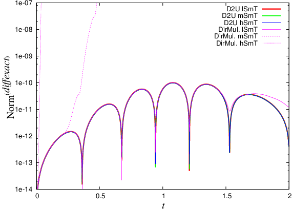
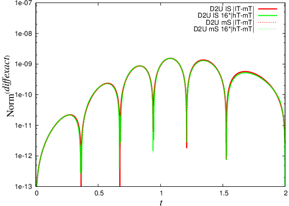
Consider Fig. 4 where we plot the deviation of the numerical from the exact solution for various resolutions and for the two different methods mentioned above. The abscissa represents time with corresponding to and to while the ordinate shows . The left plot is devoted to show these errors for a given time resolution mT, namely with time step , but for varying spatial resolutions lS , , mS , , hS , . Here is the number of collocation points in the -direction and the number in the -direction. Note that the “spiky features” in the plot just represent the oscillatority behavior of the exact solution. In the right plot we show convergence for varying time resolutions; here in addition to mT above we have lT and hT . In both plots it is obvious that the down-to-up method works very well. The absolute agreement with the exact solution is of the order . The left plot implies that there is basically no difference when the spatial resolution is changed which is clear since the solution consists only of basis functions with and is hence, up to round-off errors, represented exactly by all three spatial resolutions, cf. Lemma 8.3. Indeed, higher spatial resolutions here can only make the numerical solution worse because higher round-off errors are introduced. However, the influence of round-off errors is not notable yet and everything is very stable including our treatment of the coordinate singularity. To drive the method instable, much higher spatial resolutions have to be used, see Fig. 6. The right plot demonstrates nice th-order convergence of the code with down-to-up in time. This means that the errors are dominated by the time discretization for both the low and medium (and in fact also for the high) spatial resolutions and then the th-order Runge-Kutta method enforces th-order convergence. What is interesting about the left picture of Fig. 4 is that the direct multiplication method, i.e. the naive way of treating the coordinate singularity, is strongly instable3434 34 Here, by “instable” we do not mean the rigorous notion of Section 12.3 but a numerical solutions which deviates from its expected behavior and blows up strongly.. Higher resolution strengthen the instability which can be explained because the spatial points get closer to the coordinate singularity.
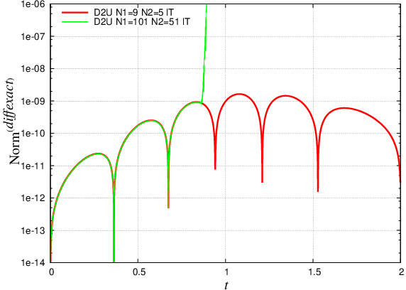

In Fig. 6 we also demonstrate convergence of the constraint violations of the linearized solution. This is actually not so easy because the initial constraint violations are of the order of the machine round-off errors and it stays like that during the evolution; hence we cannot expect to find a converging constraint violation since round-off errors spoil convergence. To see convergence of the constraints at all we introduced an artificial constraint violation of the order for the runs underlying Fig. 6. The constraint propagation system implies that the constraint violations are oscillatory in this simple case. However, even for that we find that the difference in the constraint violation for the various resolutions above is also of the order of the round-off error and still no convergence can be observed. Hence, these runs (and only the runs for this plot) are done at very low time resolutions; here lT , mT , hT , hhT while spatial resolutions are as above. Then, we are able to observe as shown in the plot, that there is th-order convergence but only for the three lower time resolutions. For the highest time resolution hhT at least the orders of magnitude are still correct. For even higher resolution no convergence at all would be visible.
This already shows a problem for the interpretation of our numerical results. Since in some applications pseudospectral methods are so accurate that round-off errors dominate, the standard convergence tests, that work very nicely for finite differencing methods in particular, have to be handled with care.

Finally consider Fig. 7 where we compare the propagation behaviors of the constraint in the linear and in the non-linear case, i.e. when the coupling between the “background part” and the spin--system is switched on again. We do this for two different spatial resolutions but with one time resolution. One can expect that the non-linear case is much more severe since the non-linear coupling induces fine structure formation. In particular, the medium spatial resolution is only sufficient at early times in the non-linear case while for the high resolution there is not very much difference between the violations in the linear and the non-linear case which means that hS is sufficient to resolve all fine structure formed. Hence, in generic non-linear runs one can expect that the demand for spatial resolution increases with time and hence it will be crucial to have some method which keeps track of this demand. A possible, and so far working approach to this is the spatial adaption method introduced in Section 15. This will be used intensively in the computation of singular spacetimes in Chapter 12. Note another typical feature from Fig. 7: the initial constraint violation is higher the higher the spatial resolution is chosen initially due to the influence of round-off errors. This has a some impact for later discussions.
23.3 Other explicit solutions
24 Regular -Gowdy spacetimes on
In this section we make numerical experiments with the methods introduced and discussed in Section 18.3 with the full non-linear evolution equations, namely the general conformal field equations in Levi-Civita conformal Gauß gauge as described in Section 10.6. As initial data on we choose a Gowdy initial data set on a Berger sphere as derived in Section 21.2 that turns out to be in the de-Sitter stability region dSSR (Section 10.8). The initial data parameters are
cf. Eqs. (124); all other vanish because we demand Gowdy symmetry. The corresponding solution turns out to be both future and past asymptotically de-Sitter, but which nevertheless has some non-trivial amount of inhomogeneity.
In this section, results from five different pseudospectral methods to compute frame derivatives on (Section 18.3) are presented and compared. The first method, referred to as “D2U Stag.” in the following plots, is the down-to-up method introduced in Section 18.3 with staggered coordinate singularities, i.e. the collocation points are shifted such that all coordinate singularities are exactly in the middle between two grid points. Correspondingly, we make the same computation with the method “D2U Non-Stag.” where the coordinate singularities coincide with the relevant grid points. We also show results of the method “D2UMod Stag.” which is just a reimplementation of the down-to-up method above but which is arranged slightly differently such that the distribution of round-off errors is not the same. We expect that the results of this method are the same as for “D2U Stag.” but the influence of round-off errors is hard to predict; eventually it turns out that there are indeed differences, see below. Furthermore, we did runs with the method “U2D Stag.” and “DirMul.”, cf. Section 18.3. For the direct multiplication method “DirMul.” the coordinate singularities are staggered between the grid points.
The runs were performed with various resolutions referred to as “lSlT” (low space low time), “lSmT” (low space medium time), “lShT” (low space high time), “mShT” (medium space high time) etc. The low resolution in time corresponds to a time step , the medium one to and the high one to . Note that corresponds to and to thus the complete spacetime is computed. The low resolution in space is , where is the number of collocation points in -direction and the number in -direction. The medium resolution in space is given by , .
It is important to note that here we do not have explicit solutions to compare with; other measures of the numerical errors have to be found. We use the violation norm of the electric constraint Eq. (126) and the following measure of the violation of Einstein’s vacuum field equations Eq. (26a)
By the -norm of a quantity we mean the sum of the -norm of and the -norms of all -derivatives of . For the tensorial quantities we additionally sum over all components as we will do in all similar expressions in the following. The physical Ricci tensor and the physical metric are projected onto the physical orthonormal frame. Since this expression is close to with the physical conformal factor, this factor is divided out. Another norm that monitors the behavior of the numerical code is introduced in Section 15; however, in this section this norm is not yet used for automatic spatial adaption. A further norm is
which gives us the order of magnitude of certain relevant components of the solution at a given time. Another error quantity measures the quality of Gowdy symmetry. As explained in Section 19.4, the symmetry along is not enforced during time evolution and there is the possibility that the solution, although initially fully Gowdy-symmetric, strongly deviates. To check this we thus define the norm
where the Killing operator is defined by
cf. Eq. (75); note that by the choice of gauge.


Consider Fig. 8. Here we plot the violation of the electric constraint vs. time for the methods above where each picture shows a fixed resolution. Exponential constraint growth, as we observe here, can be expected in most free evolutions so the questions are rather, first, how strong this growth is, second, if the violations stays small enough for the relevant time interval such that the solution can be trusted, and third, what the main reason for the growth is. The down-to-up variants all work very well and are stable. There is no difference if the coordinate singularity is staggered or not as expected. For the highest resolution the modified down-to-up method “D2U Mod” is a bit worse which shows that the influence of round-off errors for different implementations of the same thing can behave quite differently. However, this method can also be considered as stable. Definitely instable are the direct multiplication and the up-to-down methods. In particular, the instability is stronger the higher the spatial resolution is. For the direct multiplication method this can be explained because the grid points get closer to the coordinate singularity for higher resolutions. For the up-to-down method, it seems to be true what we suspected already in Section 18.3: the round-off errors which are relatively strong in high frequencies get distributed to the low frequencies and this drives instability. Hence, these two methods can be considered as unusable. Increasing the time resolution yields a smaller constraint violation at least for low times; we check for convergence in Fig. 9. As we have already seen in Fig. 7 the errors for later times can be dominated by a lack in spatial resolution, in particular for such fixed resolution runs. This results in oscillations and we can observe in Fig. 8 that their amplitudes are smaller the higher the spatial resolution is. Comparing the late time behavior of the third and the fourth plot it can be seen that the mean magnitude of the constraint violations does not change although the time resolution increases. This gives us another hint that error quantities in pseudospectral codes must sometimes be interpreted differently than in finite-differencing approaches. The problem is the following. Constraint violations of the Bianchi system are propagated by means of an homogeneous symmetric hyperbolic system of equations, the subsidiary system (Section 4). In particular, if the constraint violations vanish initially, they will vanish for all times. But in a pseudospectral code, the initial constraint violation is of the order of the machine precision, which is not zero, and hence the corresponding solution of the subsidiary system does not vanish. In fact, depending on the properties of the evolution system, the constraints do typically grow exponentially in time. Hence, from some resolution on, the constraint violations cannot be decreased anymore by increasing the resolution since the ‘‘true’’ solution of the subsidiary system with initial data of the order of machine precision gets resolved. In fact then, increasing the resolution, increases the initial data for the constraint quantities which yields an even higher constraint violations as the corresponding solution of the subsidiary system. In any case, since practically we cannot increase the machine precision3535 35 The machine precision can indeed be increased but only with a significant loss of performance., the only possibility that is left is to decrease the actual solution of the constraint propagation system by changing the properties of the evolution system. In the most prominent formulations of Einstein’s field equations, there are attempts to introduce so called constraint damping terms into the evolution system such that the corresponding constraint propagation system drives the constraint violations to zero; for instance [33, 84]. However, similar techniques have not been applied to the Bianchi system yet although there are analyses of the constraint propagation in [61]. In any case, what we can see here is that given high enough resolution, our method is able to approximate the actual solution of the subsidiary system quite accurately. With such resolutions the constraint errors and the round-off errors, but not the discretization error, dominate the errors of the solution.


The discussion of Fig. 9 is related. Here we plot again the behavior of constraint violations versus time, but we restrict to the three stable methods. In each of the two plots the spatial resolution is fixed while we vary the time resolution. Although it is not explicitly checked in this plots, we find th-order convergence for low times. The same phenomena observed as before, that for later times the spatial discretization contributes to the errors, can be observed and this results in oscillations.

Related to this is Fig. 10 where we show the behavior of the adaption norm. Recall again that adaption is not used in these runs; hence the apparent dynamics in this norm is caused exclusively by the same oscillations which we have also seen in the other norms. We see, as expected, that for low spatial resolutions, approximately independent of the time resolution, the amount of power in the high frequencies is quite high at later times and the aliasing effect (Section 12.1) is then responsible for these oscillations. For higher spatial resolutions, the power in the high frequencies is correspondingly smaller and hence the aliasing effect is not dominant.


As we discussed before, the ability to use as an error monitor quantity has limitations. That is why we also discuss the behavior of for all the methods above in Fig. 11. This error quantity measures the error in the standard ADM evolution and constraint equations (Section 4). In fact, the electric constraint corresponding to the quantity is only one of a large number of constraints in our formulation of the field equations, and it is one differential order higher than the standard ones included in . It is difficult to understand how all these constraints somehow sum up to the standard constraints. To measure these higher order errors, the first spatial derivatives of the deviations from Einstein’s field equations are included by the -norm. Now, have a look at Fig. 11. One sees that all methods agree for some time then suddenly, dependent on the spatial resolution, the direct multiplication method and later also the up-to-down method strongly deviate. What is surprising is that in the plots before we saw the two instable methods to deviate much earlier and much stronger.

To obtain some deeper understanding look at Fig. 12. There we see that the deviation of happens at that time when gets higher than the order of magnitude of the solution itself, represented by . Hence, in this sense, is on the one hand much less sensitive to errors than but on the other hand indicates when the errors really begin to dominate the solution. This should be of general interest since the standard constraints included in are the typical error monitors in numerical relativity.


In Fig. 14 we show convergence of . The errors induced by time discretization seem to play the dominant role for and we find th-order convergence for all times.
In Fig. 14 we show the behavior of . We have already explained above that the code does not explicitly enforce the invariance along , and one cannot exclude that numerical errors together with possible non-linear instabilities of the continuum evolution equations drive the solution away from this symmetry. This plot shows that this does not seem to be the case. The violation of the symmetry is a bit stronger when the resolution is higher but this is to some degree also caused by the higher round-off errors in the spatial derivative that one has to take to compute . Although these investigations here cannot be considered as systematic this result gives us indeed a hint that there is not a strong non-linear instability of the class of Gowdy solutions within the class of -symmetric solutions. We come back to this later.
Another interesting experiment, which could have been done, is to give data on , compute, as we did here, for the corresponding solution the data on backward in time, next use that data as new initial data on and finally compute the corresponding data on forward in time. The difference of the original data and the resulting data on , which would be zero in an exact solution, can be interpreted as another error measure. Further it would be interesting if those oscillations, visible for instance in in Fig. 9 caused by a lack of spatial resolution, would start close to and would stop when is approached in the same way as we have observed here.
In Section 27 we discuss some implications of our results here and of the following chapter in comparison with the existing numerical methods for the Gowdy class of spacetimes.
Chapter 12 Singular -Gowdy spacetimes
In Section 24 we computed regular -Gowdy spacetimes with spatial -topology. In particular, these spacetimes are geodesically complete and there is no curvature singularity. Here we want to compute and analyze FAdS -Gowdy spacetimes that are past singular by modifying the initial data parameters such that the de-Sitter stability region (Section 10.9) is left. While the regular class excludes the -topology, see the singularity theorems in Section 10.4, in the singular class both - and -topologies are allowed and will be studied here.
As the reader can imagine, the singular class is much more difficult to study technically than the regular class. Our results should be considered to a large degree as tests of our method, both the numerical approach and the formulations of the field equations, to find out the strengths and limitations. However, we also present some preliminary results of fundamental interest together with their investigations and discussions. In the first section we show numerical results for the conformal field equations in the Levi-Civita conformal Gauß gauge (Section 10.6) with -topology. Here the Gowdy symmetry is used to reduce the evolution equations to a -form explicitly. In the second section, similar investigations are presented for the case of -topology; note again that up to now the code is reduced only to as explained before. -simulations in the -case have not been tried yet but are expected to behave similarly as in the -case.
In the -case the solutions can be considered as non-linear perturbations of -Taub-NUT spacetimes (Section 10.2.2) and there are, in the special case considered, indications for an interesting stability of the Taub-NUT Cauchy horizon; however, the investigations have not been thorough enough yet. Further we reconsider the non-linear stability issue of the class of Gowdy spacetimes within the class of -symmetric spacetimes, which already came up in Section 24. Afterwards, we do numerical investigations with the commutator field equations introduced in Section 6. Note again, that this system is currently restricted to -topology.
25 Runs with the GCFE in Levi-Civita conformal Gauß gauge
25.1 Runs with -topology
This section is devoted to the study of numerically generated singular -Gowdy spacetimes with spatial -topology. We make use of the initial data constructed in Section 21.4 with the following two choices:
- (i)
non-polarized data
- (ii)
polarized data
As before, we assume that the other initial data quantities are given to induce the Levi-Civita conformal Gauß gauge, with the initial hypersurface . The time would correspond to but due to the singularity theorems in Section 10.4, a smooth cannot exist.


Let us start with the spacetime corresponding to the non-polarized initial data. It turns out that at the variables in the equations blow up. It is a curvature singularity because the Kretschmann scalar is divergent, see Fig. 16. In these runs, we employ our adaption techniques explained in Section 15 as one can see in Fig. 16. There, the time axis is exponentially stretched and one sees that the demand for spatial resolution increases almost exponentially in time. The runs were done with several resolutions. The resolution, which we refer to as hShT, starts from and and stops at the final time with and making use of the adaption methods described before. For the other resolutions, the automatic adaption mechanism is switched off and the adaption history of the hShT run is copied, on the one hand with half of the spatial resolution for the lShT run, and other other hand with half the time resolution for the hSmT run etc. Here is the number of collocation points in direction. Recall that these runs are .


Fig. 17 shows error norms for the runs for the resolutions above. On the left and on the right are plotted vs. time. From the left plot we can deduce that for the high spatial resolution the error is dominated by the time discretization for low times as before. For larger times, increasing the time resolution stops to make a difference. This is so because on the one hand spatial discretization plays a bigger role for later times despite of the adaption; however, apparently the aliasing effect is not dominant since no oscillations in the error norms can be observed. On the other hand, the constraint error cannot be made smaller than the actual solution of the subsidiary system as we have discussed before. Hence, so far, everything is in agreement with the results we found before. The low spatial resolution is surely not enough and we see large errors in the constraint although the code is still stable. For the other runs, one should note that although the constraint violation gets to the order at the final time, the relevant quantities of the unknowns are of the order (as we do not show here), and this means that our accuracy is of the order . This is in agreement with at the final time. As before, is much less sensible for errors caused by spatial discretization.


In Fig. 18 we plot the spatial distribution of some geometric quantities for the singular -Gowdy solutions for three different times close to the singularity. In Fig. 18a we see how the orbit volume density behaves. The orbit volume density is defined as the square root of the determinant of the matrix with , i.e. it is, to be precise, the conformal orbit volume density; but note that close to there is not much difference between conformal and physical quantities. Here one sees one particular drawback of the Levi-Civita conformal Gauß gauge compared to areal gauge. In the latter gauge, the orbit volume density is a constant on each slice and hence the singularity is approached in a “homogeneous” way. This is not the case for our gauge here and this “inhomogeneity” is even increased the further the singularity is approached. Some points, namely those where intuitively gravity is stronger, are pulled faster to the singularity than other points. In any case, such a behavior can be expected from a Gauß like gauge as ours. In Fig. 18b, where we plot the physical Kretschmann scalar according to Eq. (78), we see that exactly at those points, which approach the singularity most quickly, the Kretschmann scalar blows up fastest. To avoid confusion note that the downward pointing “spiky features” in this plot are caused by the fact the I plot the absolute value of the Kretschmann scalar and the ordinate is logarithmic. The plot Fig. 18c shows the scalar product of the killing vector fields, i.e. which are related to the quantity in the standard parametrization of the Gowdy metric. Hence one sees that this solution is definitely not polarized. Finally, in Fig. 18d we show the hyperbolic velocity, cf. Section 9.5. This is computed from Eq. (84) by first computing from our unknowns an orthonormal frame as in Section 6.3 and then by computing the relevant rescaled quantities. One sees that the velocity nearly becomes constant in time which is a hint that we are not approaching spiky features in the sense of Section 9.5.
There are further reasons to believe that the upward pointing “spiky” features in Fig. 18b are just artifacts of the gauge. A simple argument is the following. Polarized Gowdy spacetimes in areal gauge cannot develop spikes which would be visible in the Kretschmann scalar due to the results in [102], meaning that the Kretschmann scalar blows up uniformly when the singularity is approached. However, the Kretschmann scalar of the polarized solution corresponding to the polarized initial data given at the beginning of this section is nearly indistinguishable from Fig. 18b, although individual variables are very different, see for instance3636 36 Note that the jumps in this plot are produced by our time adaption method described in Section 15, since we plot the unrescaled quantities here, and hence are not geometric. Fig. 19. The relative deviation is of the order at the final time. In particular, the same upward pointing features in the Kretschmann scalar can be observed. This is a hint that the cause of these features is the “inhomogeneous” approach to the singularity in our gauge. However, we also cannot exclude the possibility that at later times, even in this gauge, “real” spikes will be visible. In any case, it would be hard to distinguish those “real” spikes from the effects that are caused by the gauge.

I should note that when I stopped the runs there were no principal numerical problems with the solutions. Indeed, the evolutions could have continued closer to the singularity. The only limiting factor so far is the constraint growth. As discussed before, I suspect that this is not caused primarily by my discretization scheme but is rather a problem either of the evolution equations at the continuum level or of the gauge. We will discuss this problem again later.
25.2 Runs with -topology
In this section we report on similar investigations in the case of -topology as before. Maybe one should note that these are the first published attempts to study -Gowdy singularities numerically. Recall from Section 19.4 that these are runs in contrast to the -case and that the ideas to reduce to have not been implemented yet. This means that we have higher practical constraints on the spatial resolution now than in the previous section. The solutions constructed here also have to be seen in relation to those in Section 24 where we chose initial in the de-Sitter stability region and hence obtained solutions which are both future and past asymptotically de-Sitter. Here now, we want to leave the stability region such that the solutions become singular in the past. All runs in this section have been done with the “D2U Stag.” method (Section 24).
Two sets of initial data as constructed in Section 21.2 are considered: Gowdy data with
- (i)
“small inhomogeneity”
- (ii)
“large inhomogeneity”
As always so far, we assume that we are in Levi-Civita conformal Gauß gauge.

It turns out that both cases appear to become singular at because some variables blow up. The behavior of the Kretschmann scalar and other quantities is discussed in a moment. As expected, the “singular” times are a bit different in the two simulations. The runs where done with the adaption mechanisms described in Section 15; Fig. 20 shows the behaviors of in both cases. The -axis has been stretched exponentially such that one can see the exponentially increasing dynamics close to the singularity in both cases. For the large inhomogeneity run, the adapted resolution, referred to as hShT, starts with , and and ends with , and . The resolutions lShT etc. are derived from that as above. Here is the number of collocation points in -direction and in -direction. For the small inhomogeneity case, the resolutions hShT starts with , and and ends with , and . The reason that the resolution for the small inhomogeneity case ended up higher than for the large inhomogeneity case – the other way around would have certainly made more sense – was my unskilful choice of representative variable to compute , namely, in both runs. From Eqs. (124) we see that the initial data parameter controls the magnitude of the initial values of . Although the initial value of was almost identical in both cases because of the definition of the norm, the consequence of this was that the time behavior of was very different in both cases. I tried to compensate this by giving different threshold values for the adaption, see again Fig. 20, however, the undesired result was that the low inhomogeneity run was done with higher resolution than the high inhomogeneity run. The fact, as discussed below, that the error quantities in the two runs are almost of identical size suggests on the one hand, that the low inhomogeneity run did not really require so much resolution, but on the other hand, that the code is also not instable when the resolution is too high (at least so far). One could have worried about this issue, cf. the investigations related to Fig. 6.


In Fig. 21 we see the behavior of some error norms vs. time in the large inhomogeneity case. The behavior is analogous to the -case before. The errors are moderate until very close to the singularity; at the end of the run is of the order and for for the hShT run. Note however that here, in contrast to the -case before, the relevant components of the solutions are of the order at the final time (as we do not show here) and hence, the relative errors indeed grow close the singularity, but are still acceptable. The suspected reason for this is the limited spatial resolution since these are -runs in contrast to -runs before. Further, it is interesting that in Fig. 21c is very stable until the errors in the solution start to grow more rapidly close to the singularity. We come back to this at the end of this section. As mentioned already above, the corresponding error quantities for the small inhomogeneity case behave very similar and thus are not plotted here.


Next consider Fig. 22 where we plot the spatial dependency of certain geometric quantities for five different times close to the singularity for the large inhomogeneity case. Corresponding plots for the small inhomogeneity case can be found in Fig. 23. Let us start with the rescaled orbit volume density3737 37 By “rescaled” we mean that the quantity is divided by as explained in Section 19.2. in Fig. 22a. Note, as in the -case, that this quantity would be constant on each slice in areal gauge, however in our gauge it is not. In the plot we shift the values of the functions such that the most right point agrees for all curves so that we can study the deformations of the curves on the way to the “singularity”. Similar to the -case, these curves deform such that points which are closer to the singularity move faster towards it which is caused by the Gauß like gauge. A similar behavior can be recognized for the small inhomogeneity case Fig. 23a. Now consider Fig. 22b which shows the spatial dependence of the physical Kretschmann scalar. We see that with increasing time a localized feature develops as we observed also in the -case in Fig. 18b. However, nothing like this is visible in the small inhomogeneity case Fig. 23b. In fact, the contrary seems to be the case there, namely the curves seem to become flatter with increasing time.
What is happening here? When the inhomogeneity parameter of the initial data, which has the value in the small inhomogeneity case and in the large inhomogeneity case, is turned to zero, the corresponding solution is a -Taub-NUT spacetime with a Cauchy horizon in the past, and expressed in our variables and gauge, some quantities, in particular the trace of the nd fundamental form, blow up there. This is so since the leaves approach a null surface. However, the Kretschmann scalar stays bounded. The behavior of the small inhomogeneity solution here shows very similar behavior indeed; for instance, the trace of the nd fundamental form blows up (which we do not show here), but the Kretschmann scalar seems to stay bounded as indicated by Fig. 23b. Now, we could speculate that the small inhomogeneity case also develops a Cauchy horizon in the past. In contrast, the large inhomogeneity case shows first signs that the Kretschmann scalar blows up, see Fig. 22b. If this speculation was true then the Cauchy horizon of the -Taub-NUT spacetime given by zero inhomogeneity parameter would be stable under small inhomogeneous Gowdy perturbations of our type. Then, the small inhomogeneity case, provided the generators of the null-hypersurface are closed, should fit into a generalization of the family of solutions in [124], and it would be interesting to find out how the relation is. There is no simple a priori way of bringing the two pictures together, since Moncrief studies the problem as a singular initial value problem with the Cauchy horizon as initial hypersurface while we start from . In any case, all this is just speculation since so far our results are not conclusive. In fact it might turn out that other curvature quantities than the Kretschmann scalar, which we do not monitor currently, blow up in the small inhomogeneity run. On the other hand, because the inhomogeneity is so small it might also be the case that the Kretschmann scalar blows up at just a little later time. In any case, a systematic study of these issues is in order. Even if it turns out that the small inhomogeneity case does not correspond to a spacetime with Cauchy horizon or that, even more, the Cauchy horizon of the corresponding -Taub-NUT spacetime is not stable under these kind of perturbations at all, it is still interesting to study the transition from our inhomogeneous spacetime family with curvature singularities to a -Taub-NUT spacetime with Cauchy horizon. Further one should investigate other classes of perturbations. The perturbations considered so far are in the Gowdy class. According to the results listed in Section 9.2 there must not be smooth Cauchy horizons in classes without symmetry. It would be interesting to study what happens when we systematically reduce the symmetry assumptions for our perturbations.
There is another remarkable aspect of Fig. 22b. The maximum of the Kretschmann scalar at the latest considered times does not correspond to the place which is closest to the singularity in contrast to the -case. We could speculate if this is a spike in the sense of Section 9.5 but further investigations of this are clearly necessary. Finally, Fig. 22c shows the scalar product of the Killing fields (similar for the small inhomogeneity) proving that the spacetime is not polarized.
Unfortunately, considerations about the interesting non-linear stability issue of the class of -Gowdy spacetimes within the class of -symmetric spacetimes had a slightly lower priority in the presentation here. What we find numerically in the singular class studied in this section, as indicated in Fig. 21c for the large inhomogeneity case, is consistent with what we found in the regular class in Section 24. Namely, the Gowdy symmetry of the numerical solutions is quite stable until the errors close to the singularity become dominant. A strong non-linear instability of the continuum equations would most likely have been visible in the numerical results. Hence, our findings indicate that such an instability is not present. Certainly, for reliable conclusions, further investigations are necessary.
26 Runs with the commutator field equations
26.1 Introduction
In the previous sections we presented some numerical calculations of singular -Gowdy spacetimes in the two cases of - and -topology using the conformal field equations in Levi-Civita conformal Gauß gauge. It turned out that this gauge is not well adapted to studies of the corresponding singularities because on the one hand the singularities are approached in a non-homogeneous way which makes interpretation of the results difficult; on the other hand the solution demands more and more resolution on time scales which become exponentially shorter when approaching the singularity. Since from previous experience we know that such problems do not occur so strongly with the commutator field equations in timelike area gauge (Section 6.3), this motivates us to start numerical experiments. Numerical results with similar equations based on finite differencing methods can be found in [10] in the case of a non-vanishing cosmological constant. Our first aim in this section is to get a feeling how well our pseudospectral approach can cope with the demands of this class of spacetimes under these “better” gauge conditions. Another aim is to deepen the fundamental understanding of the Gowdy case with non-vanishing by direct comparisons with the -case. Indeed, the investigations in the following are, to my knowledge, the only published numerical attempts to treat the Gowdy case with . However, due to time constraints in this thesis work, I only computed one numerical result regarding this issue which I present here, and otherwise just elaborate on my expectations. We start off by discussing suitable error analysis and error monitoring for this system.
Unfortunately the formulation of the commutator field equations is restricted to the case of -topology and the modification to -topology is outstanding.
Note that the solutions considered in this section are the only ones in this thesis which are not necessarily FAdS. This is so because we give data on standard Cauchy surfaces, and this yields no direct control about the evolution behavior. For , corresponding solutions cannot be FAdS anyway. In the following let us choose the time orientation such that the solutions collapse into the future, as determined by the timelike area gauge with positive and increasing time .
26.2 Error analysis and monitoring
In Chapter 11 we obtained some preliminary experience on the numerical behavior of the conformal field equations and fixed a few error quantities that we monitored in the discussion which followed. Since the situation is a bit different for the commutator field equations, this section is devoted to the discussion of some error quantities for these equations.
Let us comment on how to judge the size of the errors involved in our numerical runs. First, this can be done as usual by convergence tests but, as explained before, their interpretation can be quite different for pseudospectral than for finite differencing codes due to the potentially strong influence of round-off errors in the first case. Second, one can monitor error quantities, in particular constraint violations. We have from Eq. (66)
with obtained from Eq. (64) with
Furthermore, we have from Eqs. (69)
The Gauß constraint Eq. (65) is solved identically since is obtained from it. However, the evolution equation for Eq. (62b)
might be violated numerically. How do we measure the violation of this equation at a given time step? There is no unique way to evaluate the partial derivatives in this equation numerically. The cleanest way, i.e. avoiding further errors which are just caused by the numerical evaluation of the partial derivatives, is to substitute the relation for from the Gauß constraint and the relation for above into this equation. Then, the equation involves time derivatives of other unknowns. With the same argument as above, it is natural to determine these values from the corresponding evolution equations whose violations at a given time step cannot be measured without introducing further distinct numerical methods. It turns out that all terms cancel and from this point of view the evolution equation for above is satisfied identically. This is no surprise since it is just a reformulation of the statement that the Gauß constraint propagates. In summary, we cannot measure the violation of the evolution equation of at a given time step without introducing further numerical methods to estimate the partial derivatives involved. In general, it is a principle that “we cannot measure errors with methods that rely on the same errors”. The usage of other numerical methods to evaluate partial derivatives introduces further errors and it is hard to distinguish if the corresponding results really represent the true error quantity or rather the errors of these further numerical methods. For our purposes, we thus ignore the evolution equation of .
Now we comment on violations of the integrability condition Eq. (70) for and define its violation as . After the same kind of manipulations as before we find
Hence, this error quantity is non-trivial, but it is explicitly determined by and so it is sufficient to monitor the quantity .
Further, we would like to check if the orbit area density given by Eq. (73) is really constant on each time slice as required by the underlying gauge conditions. We define the following error quantity
and want to check if it is zero. The same kind of manipulations as above lead to
Hence, monitoring the quantities and is sufficient to estimate the error quantity .
In summary, it is sufficient to monitor the following “constraint violation” quantity in our computations which is the sum of the -norms of the quantities , , and .
For the following runs, it turns out that no time adaption is needed. This can be expected since the gauge is chosen such that the singularity lies at in an “exponential manner”; see the discussion associated with the choice of lapse in Eq. (71). A typical plot of the adaption norm is Fig. 25, where one can see that the need for spatial resolutions indeed increases in time, but not on shorter and shorter time scales as in the runs before.
26.3 Numerical Results
As initial data for the -normalized quantities (Section 6.3) we pick
which so far agrees with those in [10] and which is in the same family of data that was already investigated in [25]. However, the residual choices are (refer to as “”) and (refer to as “”) which both satisfy the constraint Eq. (66). Furthermore, the initial data for the residual decoupled part is
which is in agreement with the constraints Eqs. (69). Note that these data imply the initial hyperbolic velocity according to Eq. (84). Further recall that due to our specific choice of , our time coordinate is related to the time coordinate in [10] by .


In Fig. 25 we see the behavior of . As indicated before due to the choice of gauge, there is no need to stretch the time axis. Certainly this subserves the quality of the numerical calculations since no “artificial” time adaption is necessary. In the following we show only results obtained with one resolution and in particular no convergence plots; the code is convergent similarly as we observed before. The time resolution is in all runs shown here and fixed; the spatial resolution starts with (number of collocation points in -direction) in both runs and ends with in the case and with in the -case. In both cases, the final time corresponds to (time coordinate in [10]). This is not very close to the singularity; note, however that there was no principal obstacle to let the runs continue.
In Fig. 25 one can see the behavior of the constraint violation as introduced in Section 26.2. We see that the constraints are surprisingly well behaved, namely they decay approximately exponentially in time. Note that these jumps in Fig. 25 are produced by the spatial adaption. Namely, the individual -norms of the violations are not exactly equal before and after an interpolation step. In any case, this is a big difference to the results which we obtained with the conformal field equations.


Now consider Fig. 26 and Fig. 27 where we plot the spatial dependence of some geometric quantities for a few time steps for the - and the -case respectively. From these plots we can follow how the solution develops localized features from smooth data. In both cases a particularly sharp feature develops at , particularly visible in the plots, but which then decays again. Comparing the plots to Fig. 10 of [10], which shows3838 38 But note that the authors of [10] use Hubble-normalized quantities so that the plots cannot be compared directly. at (), we see that there is indeed no “final” spike at . Those can be observed more on the left and symmetrically on the right of and we can speculate that our plots show the early stages of such in both cases and . Consider also Fig. 26c which has little peaks at those expected positions. But why does the feature at decay in both cases? It is a “high velocity spike” [80] since its initial hyperbolic velocity is bigger than . The phenomenology of these features can be described roughly as follows. The evolution equations drive them to lower velocity while some of them (as in our case) decay completely. In [80], is assumed but in this special case here we see that the presence of does not change this behavior very much. However, the cosmological constant seems to lead to faster decay. An intuitive argument for this is that the repulsive forces of the cosmological constant blow up the localized features. Consider Fig. 25 again. Here we can follow the formation and decay of this intermediate spiky feature in frequency space. We see that the fine structure is built in short phases, shorter for , with relaxation phases in between. This is consistent with the investigations of [80] where the conclusion was drawn that the high velocity spikes decay by bouncing from one velocity regime to the next lower, while in between there are phases of relatively weak dynamics. In any case, we can see that plotting is not only interesting to study, how the code itself behaves, but also how the solution develops. This is so since building fine structure requires higher resolutions and this is represented well in Fourier space. Indeed, one can view this as an advantage of pseudospectral methods compared to other methods because the role of frequency space, in which part of the relevant information about fine structure can be read off directly, plays a fundamental role for the method itself.
These intermediate “spikes” demand quite high spatial resolutions already after a short time. But after that, when these spikes have decayed again, the resolution is not needed anymore at least for some time. The current implementation of my spatial adaption method cannot cope with this situation very well; in particular it is not able to reduce the resolution when it is not needed anymore. However, it should be straight forward to modify the method to make this possible. In any case, these intermediate spikes make my runs quite slow already after short time. Although the runs are not yet impractically slow I stopped them so that I was not able to study the final distribution of the spikes. Another reason for stopping the runs is that the current implementation of the code produces much output data, of the order of GByte, and the hard disk that I was using ran out of free space.


However, since the intermediate spikes are caused by the high velocity of my choice of initial data sets, I also computed the solution of another choice of initial data with lower initial velocity. This choice is the same as above but and , so that the initial hyperbolic velocity is . In the corresponding Fig. 28 we see that there is actually a spike at (and also at ) which does not decay and we can see its development exemplary for . Note, that the time scales are different for these data than before and we stopped the code at . The final spatial resolution was .
26.4 Expectations regarding
The numerical studies before cannot be considered as systematic investigations of the influence of the cosmological constant in solutions with Gowdy symmetry. The only aspect we could see is that maybe supports the decay of high velocity spikes. But what about low velocity spikes? Could there be an extreme value of such that all spikes decay before the singularity?
The only analytical results known so far for -Gowdy with are due to Clausen and Isenberg [51] who prove that the maximal Cauchy development of any smooth Gowdy initial data on a standard Cauchy surface is globally covered by areal coordinates where the orbit area lies in the interval for some undetermined constant . Furthermore, by means of Fuchsian methods as in [107] they obtain that one can construct solutions which are asymptotically velocity dominated in the analytic case. However, one does not obtain control over the full set of free functions.
We can say a little more than this, although many of the following arguments are heuristic. Eq. (72g) for tells us that
when we exclude the fixpoint solution (de-Sitter spacetime). Then, with , Eq. (72b) implies that
Consider the following initial value problem
A unique solution exists which has the explicit form
with . The solution exists for all if and only if . If , for . Now since, is a subsolution of this problem it follows from the standard theory of ODEs that for we have for . If we can only deduce that for all . Now for for late we can expect from Eq. (72a) that for and hence decays exponentially faster than . Since roughly speaking, the decay of is responsible for bringing the solution into the asymptotically velocity dominated regime and also for spiky features we can expect the same phenomenology as in the -case, at least if .
What about very large ? If it is initially large compared to the other unknowns then . Using this in the evolution equation Eq. (72b) implies
which has a solution that is unbounded after finite time. Let us assume that the other unknowns are so small initially such that in particular the quadratic terms can be neglected. Then all of the evolution equations are of the form for a generic unknown . Comparing this with the equation for this could mean that all these quantities increase with the same strength such that the approximation is still valid for later times. Then the whole solution could blow up after finite time. However, it is not clear in particular how the non-linear terms in the evolution equations behave in this situation. If it turns out that the other unknowns grow faster initially than , then would become more and more positive and the grow of would be damped such that possibly the solution stays finite for all times. In any case, what I want to say by means of this heuristic discussion is that is not easy, without usage of more difficult arguments, to exclude a blow up after finite time if the is high enough initially. Such a blow up would imply a drastic change in the dynamics for compared to the well known case. This possibility is maybe related to the outstanding issues in the theorems by Clausen et al. explained above. Can the constant always be chosen to be zero? As we said, for “small enough”, this can be done. But if not, what kind of singular behavior is there? Note, that if the solution is, say, past asymptotically de-Sitter (past decreasing the -coordinate), then all timelike geodesics are future incomplete in this case, at least when the scalar curvature of is negative, due to the singularity theorems of Section 10.4. But do they run into curvature singularities or Cauchy horizons? In the first case: are the solution in some sense asymptotically velocity dominated? Recall, that Clausen et al. were not able to prove that all solutions are asymptotically velocity dominated, not even in the analytic case.
Chapter 13 Conclusions, projects for future research and summary
Having described the ideas underlying my method and its implementation in Part II and discussed the analysis of several application problems in Part III, we now want to conclude and summarize. We start this chapter with Section 27, where we conclude about the technical properties of my method with emphasis on the restricted set of applications in this thesis. For these discussions the technical results presented in the previous chapters are taken into account. Then, in Section 28, we describe open problems of both technical and physical-mathematical nature. On the one hand, we reconsider the preliminary results about properties of the solution space of EFE obtained in this thesis, and, on the other hand, we discuss expectations about other applications of interest which particularly go beyond the limited set of applications considered in this thesis. At the end of this chapter, in Section 29, we summarize.
27 Conclusions about the numerical method
The purpose of this section is to compare my method to those listed in Section 13 and to draw some conclusions. In agreement with our previous analysis, we focus on two aspects here, namely first, the way my code is able to cope with the presence of the coordinate singularities of the Euler parametrization of , and second, how well it allows to approach Gowdy singularities. It should be clear that for -Gowdy spacetimes these aspects cannot be discussed independently. Recall the definitions of the various pseudospectral techniques to deal with the coordinate singularity in Section 18.3.
In Section 23.1 we analyzed the linearized GCFEs on the de-Sitter background and found that the down-to-up treatment of the coordinate singularity is stable and reliable. Similar results were obtained in Section 24 where we considered non-linear regular -Gowdy solutions. In particular, there was no notable difference between staggered and non-staggered coordinate singularities; both performed equally well. Further investigations of singular -Gowdy spacetimes with -topology in Section 25.2 supported the conclusion that the coordinate singularity treatment introduced in this thesis works quite well.
However, in these investigations we also found that both our direct multiplication and up-to-down methods are instable. Although it is in principle clear that round-off errors are responsible for that, in particular for the direct multiplication method which is implemented without any projection, we have no real understanding of the mechanisms. Conversely, the same can be said about the stability of the down-to-up method. This issue is not restricted to our situation here. Indeed, similar observations are made for the axis singularities of cylindrical coordinates in . Note that the coordinate singularity on resembles these singularities. In the case of axis singularities, important contributions are the implementations (Section 13.1) by Garfinkle et al. [77, 79], the one by Choptuik et al. [38] and that by Rinne and Stewart [153, 154]. With the exception of [77], all those assume axisymmetry. The implementations by Garfinkle et al. and Choptuik et al. are similar to our direct multiplication. Namely, at the staggered coordinate singularity, one multiplies “directly” functions with a zero, in particular some of the variables possibly after clever rescalings, with functions having a pole, in particular singular terms in the equations. If the initial data are chosen appropriately, the (exact) evolution equations imply that the variables decay with the right order at the singular points at all times such that the limit of such products is finite. However, the discretized equations can be instable. This is the reason why in the methods above the problem is formulated as an initial boundary value problem, and boundary conditions necessary for smoothness are prescribed to yield at least some sort of control there. However, there is still the possibility that the solution of the discretized equations behaves in an undesired manner at the boundary. Indeed, Choptuik et al. find that even with such boundary conditions, their code is instable at the axis, and they have to use Kreiss-Oliger dissipation to cure this. In contrast to that the approaches by Garfinkle et al. are reported to be stable. Since the reason for this different behavior is not known, we can state that the issue of axis instabilities is not understood in general. The implementation by Rinne and Stewart is a bit different because they were able to find a formulation of the equations which is completely free of singular terms in the axisymmetric case. In particular their evolutions are claimed to be stable at the axis. However, it is unclear if their treatment can be generalized to cases without axisymmetry. In general, one can expect that, at least to some degree, the choice of the time-marching scheme has an impact on this stability issue because certain schemes have higher implicit dissipation than others, but to my knowledge this has not been investigated systematically yet. In particular it would be interesting to experiment with other time integrators than Runge-Kutta in my code.
Indeed, there is a further motivation for experiments with other time-marching schemes which is particularly relevant for spectral methods. Since the evaluation of the spatial derivatives of all variables on a given time slice is relatively expensive for spectral methods, one should look for time-marching schemes which take as few trial time steps as possible for each time step. In particular, it may be possible to find a better compromise between speed and stability than the th-order Runge Kutta scheme used in this thesis.
To conclude, if we want to treat a situation with a coordinate axis singularity numerically, not necessarily with axisymmetry, in which spectral methods are appropriate then the experience in this thesis suggest that an approach based on our down-to-up method is highly accurate, stable and reliable. However, when applications are studied for which spectral methods cannot be expected to be optimal then one might have to consider something else; for instance one of the other techniques mentioned here. In any case, a description of the mechanisms driving instabilities derived from first principles is outstanding.
This suggests that for the discussion of our second focus, namely the approach to the Gowdy singularity, we must clarify to which extend spectral methods are appropriate, or if finite differencing are favorable. For a fair comparison with other treatments of Gowdy spacetimes, we should point out that the problems which we observed in Section 25.2 to approach the singularity in -Gowdy spacetimes are believed to be caused to a large degree by the unsuitable choice of gauge. Further, the constraint growth in our reduction of the conformal field equations was very strong. However, we are optimistic that one can find a modification of the commutator field equations for the -case and a -reduction according to the ideas in Section 19.4, such that we can use our techniques for the -Gowdy problem in timelike area gauge. Our experience with the spectral code to treat the -Gowdy case with the commutator field equations in Section 26 shows that a few thousand grid points are in reach of the method. This is the order of magnitude of grid points that was also used by Garfinkle in [77] to treat the -case. He was able to achieve accuracies of the order and shows results up to time where in his convention the orbit area density is proportional to and . With our pseudospectral approach and with the expected formulation of the problem as above, one could hence reach at least as much accuracy in the -case; it is likely that the accuracy is even higher due to spectral discretization. However, we can also expect that resolutions of this order of magnitude would constitute a limit for our method, at least without further technical devices like local adaption or parallelization.
We have seen that for our method, adaption is crucial to approach the Gowdy singularity. In the timelike area gauge, as we experienced in Section 26, adaption is not needed in time but certainly in space. Fixed resolution codes, as for example the one by Berger and Moncrief [25], have to use very high resolution right from the beginning; for example they made runs with grid points in space and were able to keep the errors below the order . However, first, such high number of grid points can probably be never reached with spectral methods, and second, even if one could reach it, one would eventually start to lose spikes when they become smaller than the grid spacing. Hence, adaption is particularly important for spectral methods, however, note that the second aspect is surely an issue for finite differencing as well. Our adaption method described in Section 15, as primitive as it may seem on the first sight, is particularly nice to track the smallest scales relevant for the solution due to our analysis in frequency space.
A further argument pro spectral methods for the approach to Gowdy spacetimes is the following. As argued in [31], it is a rule-of-thumb that in general spectral methods have lower implicit dissipation than most finite differencing discretizations. Too high dissipation can influence the evolution of localized features drastically as been experienced by Hern et al. [91] with their Lax-Wendroff scheme. Since this feature of pseudospectral methods is dependent on the choice of the time integrator, we have thus found another motivation to experiment with other time-marching schemes for optimizing the dissipative character of the method.
For further conclusions one should start direct comparisons of all relevant techniques systematically. In the single patch case, changing from pseudospectral discretization to finite differencing is in fact straight forward the way my code is implemented. For multi-block techniques, it is likely that a new code has to be created based on the already existing infrastructure of [56]. However, these methods are particularly promising not only due to their generality, but in particular also because the existing infrastructure offers efficient parallelization on super computers and fixed mesh refinement.
The hope that motivated me to use pseudospectral methods is so far well supported by the numerical experiments done in this thesis. Coordinate singularities can be treated in a clean way without having to rely on complicated multipatch methods. Indeed, it is realistic to believe that sufficient resolutions to treat the -Gowdy case are in reach of the method which could give us all advantages which a spectral method has to offer. For this, it is crucial to find a reliable way of formulating the timelike area gauge in a -fashion. As soon as this is possible, the method presented in this thesis should be able to treat the so far outstanding case of Gowdy solutions with -topology with resolutions as in Garfinkle’s work about the -case. I should point out that the current implementation of my code is not yet optimized for efficiency, on the one hand because I am not yet using the FFT algorithm, and on the other hand because I am not yet taking into account the special structure of the Fourier series in the -case. These possibilities make it even more likely that sufficient resolutions can be reached. However, we can also expect that my method, in its current form, is not able to reach more resolution than this; further discussions on this aspect can be found in the next section.
It should be clear that these results of this thesis, which focused on two main aspects, do not allow to draw real conclusions about the applicability of our method, neither in the positive nor in the negative sense, when one wants to go “beyond” Gowdy or treat other problems of interest. However, certainly one can formulate some expectations. A discussion on modifications which are expected to become necessary can be found in Section 28. In particular, for Gowdy solutions the problem is simplified by the fact that a nicely adapted gauge is known, namely the timelike area gauge. But which gauge to choose in more general situations? See [78] and references therein for some ideas. Further, in Gowdy solutions one observes no oscillations close to the singularity. In general, according to the BKL-conjecture, such difficult phenomena can be expected and the numerical method must be adjusted to be able to cope with these. Some ideas on this can be found in [23, 19]. Further it might turn out that in general we find pathologies even more severe than spikes. Those would certainly require even more sophisticated local adaption techniques. For other applications than the cosmological singularities we list further ideas in the next section.
28 Outstanding issues and future research projects
I will now summarize problems that were left open in this thesis, further interesting application projects and possibly necessary modifications of my method. All these aspects could be among my future research topics. In accordance to what we have stated before, we discuss the questions of interest in connection with our expectations about the required techniques in the following.
Gravitational singularities
In Section 27 we have already drawn some conclusions on the properties of the current implementation of my code regarding the two main issues of this thesis, namely the coordinate singularity of and the approach to Gowdy singularities, both in comparison with other methods on the market. Here we continue this discussion with the particular emphasis on future research possibilities.
Certainly, an important future research project will be to continue the investigations of past singular -Gowdy solutions with -topology started in this thesis. In a first step one can ignore the issue of constructing FAdS solutions. Recall that it is conjectured that the singularity is asymptotically velocity dominated with similar types of spikes as in the -case. For the -case, this conjecture is supported by the numerical results in [77]. The only relevant analytical results of [102, 159] cannot be considered as complete. A bit farther in the future, we also want to study issues like cosmic censorship and the BKL-conjecture for more general cases, for example in -symmetry. In principle my code in its current form could be applied in this situation. In an even farther future, we would like to give up all symmetry assumptions to study “generic singularities” and continue the research program started in [78]. In that work, the topology is restricted to and it would be interesting if similar statements can be obtained in the -case in particular. Up to now in the -case, my code was implemented assuming -symmetry. In order to use it for studies of spacetimes without any symmetries, our analysis of the coordinate singularity has to be generalized. I expect no principal problems with this, only that all expressions in Chapter 8 become more complicated.
I have already stated that I am optimistic to reach sufficient resolutions with my code to study the -Gowdy case, if it turns out to be possible to formulate the equations in a -fashion with timelike area gauge. For this problem it seems worthwhile to try to adapt the commutator field equations to the -case since this system seems to be well-behaved in our experiments in Section 26. We are also optimistic that the problem can be reduced to even in the -case due to the ideas in Section 19.4. That general optimism is particularly based on the expectation that my global spatial adaption technique (Section 15) is sufficient to study Gowdy singularities. However, for future studies, either when the localized features become more complicated than Gowdy spikes in more general situations, or when computer resources have to be handled more efficiently, one must start to think about local adaption techniques. For instance, I expect that without such techniques my current implementation is limited practically to a few thousand spatial grid points in . With finite differencing, implementing such local adaption techniques is not as difficult as in spectral methods. Nevertheless, pseudospectral multidomain approaches, which can be used for fixed mesh refinement, have been implemented successfully in numerical relativity; for elliptic equations see [138, 11], for the hyperbolic “generalized harmonic” formulation of EFE applied to the binary black hole problem see [156] and for a special mixed elliptic-hyperbolic problem see [109].
In any case, there are several motivations to compare the method worked out in this thesis to other numerical methods directly, both in the -case without coordinate singularities and in the -case. First, it is always important to compare the differences of the results obtained from distinct numerical techniques to get further insights into the errors involved. Second, despite the better accuracy property, high resolution spectral approaches are usually more expensive than finite differencing methods with the same number of grid points. This is the basis for the expectation that finite differencing discretizations may cope better with small scale features, as those close to gravitational singularities. To switch our code to finite differencing is, at least on , straight forward. The issue how finite differencing is able to deal with the coordinate singularity on is outstanding. In systematic comparisons of different methods the multi-block approach [56], see Section 13.1, should play a major role. This should be so not only because of its generality but also because the existing numerical infrastructure of these codes, involving efficient parallelization routines to put runs onto supercomputer and fixed mesh refinement, may become necessary as has already been argued above. Codes based on pseudospectral methods and FFT can also be parallelized in principle, for instance the implementation [74] of FFT supports this, but it cannot be expected that this is as efficient on computer clusters of standard type as in the finite differencing case.
In any case, our current implementation is not optimized for efficiency. On the one hand the partial summation method (Section 14) should be substituted by FFT, either by using one of the freely available highly optimized libraries (e.g. [74]) or by implementing it individually. The code will benefit from this in particular for the high spatial resolutions needed at gravitational singularities. Further, in the -case we should make use of the special properties of the Fourier series involved to reduce the amount of computations in each time step. Another important aspect is that my code does not yet handle output data in an efficient way. The runs which I presented before in this thesis produced a couple of GBytes of data in total which caused hard disk space problems.
If the BKL-conjecture is true, the Gowdy singularity is exceptional since it is asymptotically velocity dominated. For other more general applications involving gravitational singularities, one can expect that the solutions behave oscillatory. This means that we must pay special attention to the implementation of the time integrators so that they can cope with this difficult problem. Ideas for this can be found in [23, 19]. Some results on this issue are available in the class of -symmetric spacetimes with non-vanishing twist constants (which is only possible on ). Also, for -symmetry, velocity dominated singularities are expected in the “polarized” case [27], while oscillatory ones show up in the “non-polarized” case [26].
With evolution systems similar to the commutator field equations to study the -Gowdy singularities, we are forced to set up the Cauchy problem with respect to a standard Cauchy surface because, as noted before, there seems to be no way of regularizing the equations on . Hence we have the problem that we cannot decide a priori from the data if the corresponding solution is FAdS. Hence, to study the singularities in FAdS -Gowdy spacetimes, one should explore the ideas to transfer data from the conformal field equations to the commutator field equations in Section 22. Assuming that this can be done, the next problem for more thorough studies of -Gowdy FAdS solutions is to construct more general or at least different classes of initial data than those derived in Section 9. In particular it will be interesting to construct a family of -Gowdy initial data that contains the polarized case to compare with the analytic results in the -case. On the one hand, this can be considered as another code check in the -case, and on the other hand, the outstanding case can be studied in this simpler setting first. We have argued before that it is an outstanding problem for all topologies if the presence of the cosmological constant can change the phenomenology of the solutions. Already in the much simpler case of -topology there are interesting expectations, in particular regarding outstanding issues of certain theorems, see Section 26.4. Indeed, with the current version of the -commutator field equations code systematic studies of these issues should be straight forward and new insights can be expected. Again regarding the initial data issue, eventually one would like to have initial data on which can be considered in some sense as generic within, say, the -Gowdy class, i.e. one should be able to give convincing arguments that the corresponding solutions include all relevant phenomena of generic solutions.
As we already said, the Gowdy case with spatial -topology is outstanding from the numerical but also from the analytical point of view. Indeed, there are, besides the analytical results for the polarized case in [102], problems in the analytical investigations in [159] in the two cases and . It would be enlightening to find out, possibly with our numerical method, if these problems are really caused by unexpected phenomenology or rather by the imperfectness of the analytical methods. Note again that being able to perform calculations in the -Gowdy case, we are also able to do calculations in the -case as argued in Chapter 6.
Studies of solutions with Cauchy horizons
In the discussion in Section 25.2 we speculated that the “small inhomogeneity” run shown there develops a Cauchy horizon in the past. However, to make conclusive statements, further investigations are necessary. If this turns out to be true then one has to find out if and how this spacetime fits into Moncrief’s class of generalized Taub-NUT spacetimes [124]. If, after all, this solution turns out rather to have a curvature singularity in the past, e.g. because the Kretschmann scalar blows up later, it could still be enlightening to study the transition from the curvature singularity of the perturbed Taub-NUT spacetime to the Cauchy horizon of the unperturbed case by systematically decreasing the inhomogeneity parameter. In the opposite direction, the general belief is that Cauchy horizons decay in some way to BKL-singularities under generic perturbations so that a real observer can never cross it. However, first, it is not clear how this transition takes place and second there are situations known with different behavior, for instance weak null singularities (Section 9.3). In any case, we should point out here that studies related to Cauchy horizons are usually very subtle. It is in general unsolved how to actually determine, in particular numerically, if a solution develops a Cauchy horizon. A first non-sufficient indication for a Cauchy horizon is that the trace of the nd fundamental form blows up, because the slicing approaches a null hypersurface, while curvature invariants are bounded. But, how do we distinguish a Cauchy horizon from a simple break down of the coordinate gauge? How do we want to conclude something about extendibility when the unknowns in the equations blow up numerically? This is indeed a problem because variables blowing up numerically without any analytical information on the type of singularity can be expected to involve large error components.
In situation for which one knows analytically that Cauchy horizons exist, there is an alternative way to study the character of the horizon and the associated spacetime. Namely, we can try to reconstruct such a solution numerically in a gauge built upon timelike congruences which, at least partly, are able to cross the horizon. Then all issues related to Cauchy horizons like instability with respect to perturbations, in particular those induced by numerical errors, local non-uniqueness and possibly the existence of closed causal curves could have an impact, and it could be interesting to see how these show up in the numerical computation. Dependent on the situation, such investigations might already be possible in the general conformal Gauß gauge since this gauge is motivated geometrically. The generalization of our current implementation which is restricted to the Levi-Civita conformal Gauß gauge (Section 10.6) to general conformal Gauß gauges is not expected to be problematic in principle. However, when we want to compute solutions as just suggested with the general conformal field equations, we have to solve or at least weaken the problem of constraint growth. Recall that our runs in Section 25 showed strong constraint growth and it seemed that this issue was the main limitation for the precision of the calculations. It might be crucial to find another reduction of the Bianchi system such that the constraint propagation is optimized.
The set dSSR and properties of corresponding solutions
We have already mentioned that there is currently not much understanding of the properties of the stability neighborhood of the de-Sitter solution, e.g. boundedness, connectedness etc. It would be interesting to obtain further insights on this and such could be obtained by means of our numerical code. This could be done by studying the initial data space systematically, for example by investigating non-linear perturbations of the -Taub-NUT family, because this family interpolates some of the relevant regions in this space.
Related to this is the following. We have studied both singular and regular -Gowdy spacetimes in Section 24 and 25 and speculated about the non-linear stability (of the continuum equations!) of this class within the class of -symmetric spacetimes. It would be interesting to continue such studies because such a stability might give us indications about the physical significance of Gowdy spacetimes. For the regular class, in particular those -Gowdy solution whose -initial data is in dSSR, the current implementation of my code seems to be well adapted to such stability studies because, apart from the constraint growth probably associated with the formulation of choice of the conformal field equations, we were able to reach high accuracy. In the singular case, i.e. when we leave the stability region, many of the technical problems above have to be considered before reliable conclusions about these stability issues can be obtained.
A very challenging class of problems is related to the construction of solutions whose initial data is at (or maybe even close to) the boundary of dSSR with partial . In this case one can expect that one has to find a gauge such that the time slices do not approach the singular parts of too closely while simultaneously covering the regular parts. Maybe it is possible to realize such a gauge within the class of conformal Gauß gauges. If we were indeed successful to construct such solutions, then we could maybe draw connections to the field of cosmological black hole physics as we have argued in Section 10.10. Namely, it might be possible that such solutions with partial in the -case fail to be asymptotically simple in a non-trivial manner. Thus they could have both collapsing and expanding regions, and this might give rise to this interpretation. One knows some families of explicit cosmological black hole solutions, for instance the Schwarzschild de-Sitter solution (Section 10.2.3); but this does not correspond to our class because neither nor are compact. Further, so far, there are not many attempts to study the space of cosmological black hole spacetime more generally. One of these attempts is [30] (see also references therein) where the class of Robinson-Trautman spacetimes with is investigated.
Other issues and applications
There are further numerical problems whose investigations can be interesting. It could be particularly enlightening to get further insights into the problem of axis instabilities which were discussed in Section 27. One way of approaching this problem is to experiment with different time-marching schemes. Such studies on how this influences both numerical dissipativity and efficiency, could be of use even for completely different numerical applications.
Another numerical problem of more fundamental kind is the following. During the analysis of my numerical experiments (Chapter 11) I pointed out that round-off errors can be an important error source and it can be expected that this is true also in other applications. To study systematically how important this error source really is, I should, besides making statistical analyses as in [105], repeat a few of my runs with “quad” precision. Up to now, I used the standard “double” precision exclusively, meaning that the numbers in the code are represented with roughly decimal digits, internally with bits. I chose “double” precision because this is the native internal precision of the processors. For “quad” precision the numbers are represented with bits which gives an accuracy up to decimal digits. But note that, quad precision numbers have to be emulated by the software, i.e. are not directly supported by the processor, and this slows down the code significantly. More information on the binary representation of floating point numbers used by the Intel compilers and processors can be found in [98]. Nevertheless, it should be sufficient to compute a few time steps in a few cases to draw further conclusions.
There is another big class of applications which seems unrelated at first sight, namely the dS-CFT correspondence which we have completely ignored in this thesis so far. The basic idea is to formulate a physical conformal field theory on the conformal boundary of a spacetime with positive Ricci curvature, and, dependent on the properties of the conformal boundary and the conformal field theory, to make statements about the properties of the conformal spacetime. The underlying concept is the holography principle [163]. The dS-CFT correspondence is the positive curvature analogue of the famous AdS-CFT correspondence [119] which was first formulated to resolve certain issues in string theory. A mathematically profound overview article is [3] and a brief description and the status of the mathematical idea can be found in the introduction of [8]. Since Friedrich’s Cauchy problem is a well-posed formulation, at least in dimensions, to study the outstanding issues of dS-CFT, investigations of open issues in this correspondence are indeed related to our discussions before.
29 Summary
Motivated by the observational evidence that our universe is in an accelerated expanding phase presently, we have studied the class of FAdS solutions of EFE in this thesis. Although these spacetimes are “almost” in accordance with the cosmic no-hair picture in the future and hence “simple” in some sense there, there is a difficult and so far not understood interrelation of the past behavior and the properties of . If the topology of is compact, then there are a number of theorems, including singularity theorems, the Yamabe theorem and stability theorems which draw a certain picture about this issue. However, this picture is both incomplete and mysterious. First, the theorems available are not able to cover all situations of interest. Second, there are major outstanding issues in general relativity which also show up here. For example it is currently not more than a hope that generic maximal globally hyperbolic past incomplete solutions are -inextendible as claimed by the strong cosmic censorship conjecture. Further it is not clear in general under which conditions curvature singularities are really of BKL-type. In the class of FAdS solutions, all these outstanding questions and problems can be expected to be influenced by a subtle interplay of the time evolution and the geometrical properties of . FAdS solutions can be constructed by means of Friedrich’s Cauchy problem involving his conformal field equations. It is a well-posed formulation of the problem which allows to prescribe -data sets subject to relatively weak constraints; in particular the topology and geometry of can be given almost freely. In this thesis, we decided to restrict to the topologies and , since these provide the simplest paradigms to shed light on these issues.
I decided to approach the outstanding issues in this class of spacetimes numerically. There are several techniques to treat spacetimes with spatial topologies as which are “non-trivial” from the numerical point of view. We started by discussing our motivation to develop a single patch approach based on pseudospectral methods and elaborated on expected advantages and disadvantages. After having motivated a choice of coordinates on , we described the development of the numerical method. Our implementation was done in a way such that spatial - and -topologies can be treated with the same spectral infrastructure; this was realized by studying a map . Consider the pull-back of a smooth function on via this map to . The special properties of its Fourier series was analyzed and the formally singular terms in the equations at the coordinate singularities were explicitly regularized in terms of Fourier expansions. Part II is devoted to the explanation of these ideas and of the implementation of the code. Afterwards in Part III, applications and their analyses are discussed.
In this thesis we restricted to applications involving spacetimes with Gowdy symmetry. The main motivation for this was to simplify the problem, however, the code is implemented such that it is not restricted to this symmetry. Gowdy symmetry was also the motivation for our choice of coordinates on . Gowdy spacetimes can be considered as one of the simplest inhomogeneous classes of solutions of EFE but which nevertheless show high complexity. Due to several rigorous results on this class of spacetimes one has a large catalog of ideas for the outstanding cases, in particular for -Gowdy solutions. With our code we were able to provide the first, though so far unsystematic, studies in the published literature of -Gowdy solutions.
In Part III, we started by investigating linearizations of the field equations and by comparing the numerical results to the known exact solutions in presence of the coordinate singularity. Then I analyzed the errors obtained with various variants of my spectral approach for (non-linear) regular -Gowdy spacetimes with -topology. In both cases I was able to identify one method which is stable and highly accurate, namely the so called down-to-up method. Next, I applied this stable method to compute singular -Gowdy spacetimes with spatial -topology, but also with -topology for comparisons. It turns out that the Levi-Civita conformal Gauß gauge used for both topologies is not suitable to approach the singularity in a “homogeneous” way. Although the results are very accurate, this did not allow us to compare our results to those obtained by means of other methods. Nevertheless, two main preliminary observations were made besides the successful testing of the implementation. The first of these results suggests that the class of -Gowdy solutions with -topology might be non-linearly stable within the class of -symmetric solutions. The second of these results has to do with the possible stability of the Cauchy horizon of a -Taub-NUT spacetime under perturbations of Gowdy symmetry. However, further discussions and analyses are necessary for reliable conclusions.
The problems related to the Levi-Civita Gauß gauge, but also the lack of understanding how a suitable gauge to approach the Gowdy singularity can be formulated for the conformal field equations, motivated us to consider the commutator field equations. These equations are so far restricted to Gowdy symmetry and -slices, however, they are formulated in the highly adapted timelike area gauge and do not require . Of course, the conformal field equations can also be applied for any sign of the cosmological constant, however, the specific formulation Eqs. (93), which I implemented, requires . Our numerical results obtained with the commutator field equations were very accurate and promising, and we were able to reproduce the fine structure at the Gowdy singularity. Indeed, these were the first published attempts to compute -Gowdy spacetimes with numerically. This case is particularly interesting as we argued and, although we have not been able to make systematic studies due to lack of time, we elaborated on our expectations related to this outstanding issue at least. Note however, that the solutions obtained with the commutator field equations so far are not necessarily FAdS.
We further argued that if we were able to implement our preliminary ideas to modify the commutator field equations for -topology in a -manner, we could reach sufficient resolutions in the Gowdy -case to obtain at least as much accuracy as Garfinkle in his work on Gowdy -solutions, but with all advantages of a spectral method.
In this thesis we have focused on two main aspects: first, the numerical construction of solutions of EFE under the presence of the coordinate singularity, and second, the numerical approach to the Gowdy singularity for the spatial topologies and . Clearly, other interesting applications, outstanding problems and questions had to be deferred. Some of those were summarized and discussed in Section 28. Although we obtained only a limited amount of results on the outstanding issues of general relativity in this thesis, the large number of possibilities for future research suggests that our investigations here have contributed to open the door for many interesting studies in the future.
In summary, the investigation of the class of FAdS spacetimes is a promising challenge both from the fundamental and the numerical point of view. A rich phenomenology with the possibility to obtain deeper insights on fundamental outstanding problems in general relativity is expected. I believe that the mutual interaction of pure mathematics and numerical treatment can be very helpful to come up with new ideas and new approaches for our research field by combining the power of these two. Maybe, by making use of the forthcoming accurate observational results, even new implications for the properties of our own universe can be derived, for instance predictions about the distribution of the temperature fluctuations in the cosmic microwave background and primordial gravitational waves.
References
- [1] M. Alcubierre. The status of numerical relativity. preprint, 2004, gr-qc/0412019.
- [2] M. Alcubierre, S. Brandt, B. Brügmann, D. Holz, E. Seidel, R. Takahashi, and J. Thornburg. Symmetry without symmetry: Numerical simulation of axisymmetric systems using Cartesian grids. Int. J. Mod. Phys., D10:273–290, 2001, gr-qc/9908012.
- [3] M.T. Anderson. Geometric aspects of the AdS/CFT correspondence. In Proceedings of the Strasbourg meeting on AdS/CFT, page 23, 2003, hep-th/0403087.
- [4] M.T. Anderson. Existence and stability of even dimensional asymptotically de Sitter spaces. Annales Henri Poincare, 6:801–820, 2005, gr-qc/0408072.
- [5] M.T. Anderson. On the structure of asymptotically de Sitter and Anti-de Sitter spaces. Adv. Theor. Math. Phys., 8:861–893, 2005, hep-th/0407087.
- [6] M.T. Anderson and P.T. Chruściel. Asymptotically simple solutions of the vacuum Einstein equations in even dimensions. Commun. Math. Phys., 260(3):557–577, 2005.
- [7] L. Andersson. The global existence problem in general relativity. In P.T. Chruściel and H. Friedrich, editors, The Einstein Equations and the Large Scale Behavior of Gravitational Fields: 50 Years of the Cauchy Problem in General Relativity, pages 71–120. Birkhäuser, Basel, Switzerland; Boston, U.S.A., 2004.
- [8] L. Andersson and G.J. Galloway. dS/CFT and spacetime topology. Adv. Theor. Math. Phys., 6:307–327, 2002, hep-th/0202161.
- [9] L. Andersson and A.D. Rendall. Quiescent cosmological singularities. Commun. Math. Phys., 218:479–511, 2001, gr-qc/0001047.
- [10] L. Andersson, H. van Elst, and C. Uggla. Gowdy phenomenology in scale-invariant variables. Class. Quant. Grav., 21:S29–S57, 2004, gr-qc/0310127.
- [11] M. Ansorg. Multi-domain spectral method for initial data of arbitrary binaries in general relativity. preprint, 2006, gr-qc/0612081.
- [12] R. Aurich, S. Lustig, F. Steiner, and H. Then. CMB alignment in multi-connected universes. Class. Quant. Grav., 24:1879–1894, 2007, astro-ph/0612308.
- [13] J.G. Baker, M. Campanelli, F. Pretorius, and Y. Zlochower. Comparisons of binary black hole merger waveforms. preprint, 2007, gr-qc/0701016.
- [14] J.G. Baker, J. Centrella, D. Choi, M. Koppitz, and J. van Meter. Gravitational wave extraction from an inspiraling configuration of merging black holes. Phys. Rev. Letters, 96:111102, 2006, gr-qc/0511103.
- [15] C. Bär. Lorentzgeometrie. University Potsdam, Lecture Notes, Summer Semester 2004, 2006, http://users.math.uni-potsdam.de/~baer/LorGeo/Skript.pdf.
- [16] R. Bartnik and J. Isenberg. The constraint equations. In P.T. Chruściel and H. Friedrich, editors, The Einstein Equations and the Large Scale Behavior of Gravitational Fields: 50 Years of the Cauchy Problem in General Relativity, pages 1–38. Birkhäuser, Basel, Switzerland; Boston, U.S.A., 2004.
- [17] V.A. Belinskii, I.M. Khalatnikov, and E.M. Lifshitz. Oscillatory approach to a singular point in the relativistic cosmology. Adv. Phys., 19:525–573, 1970.
- [18] V.A. Belinskii, I.M. Khalatnikov, and E.M. Lifshitz. A general solution of the einstein equations with a time singularity. Adv. Phys., 31:639–667, 1982.
- [19] B.K. Berger. Numerical approaches to spacetime singularities. Living Reviews in Relativity, 5(1), 2002, http://www.livingreviews.org/lrr-2002-1.
- [20] B.K. Berger and D. Garfinkle. Phenomenology of the Gowdy universe on . Phys. Rev. D, 57:4767–4777, 1998, gr-qc/9710102.
- [21] B.K. Berger, D. Garfinkle, J. Isenberg, V. Moncrief, and M.J. Weaver. The singularity in generic gravitational collapse is spacelike, local and oscillatory. Mod. Phys. Lett. A, 13:1565–1574, 1998.
- [22] B.K. Berger, D. Garfinkle, and V. Moncrief. Comment on “The Gowdy cosmologies revisited”. comment preprint, 1997, gr-qc/9708050.
- [23] B.K. Berger, D. Garfinkle, and E. Strasser. New Algorithm for Mixmaster Dynamics. Class. Quant. Grav., 14:L29–L36, 1997, gr-qc/9609072.
- [24] B.K. Berger, J. Isenberg, and M.J. Weaver. Oscillatory approach to the singularity in vacuum spacetimes with isometry. Phys. Rev. D, 64:084006, 2001, gr-qc/0104048.
- [25] B.K. Berger and V. Moncrief. Numerical investigation of cosmological singularities. Phys. Rev. D, 48:4676–4687, 1993, gr-qc/9307032.
- [26] B.K. Berger and V. Moncrief. Evidence for an oscillatory singularity in generic symmetric cosmologies on . Phys. Rev. D, 58:064023, 1998, gr-qc/9804085.
- [27] B.K. Berger and V. Moncrief. Numerical evidence that the singularity in polarized symmetric cosmologies on is velocity dominated. Phys. Rev. D, 57:7235–7240, 1998, gr-qc/9801078.
- [28] M. Berger. Geometry, volume 1. Springer, 2nd edition, 1994.
- [29] M. Berger. Geometry, volume 2. Springer, 2nd edition, 1996.
- [30] J. Bičák and J. Podolský. Cosmic no-hair conjecture and black-hole formation: An exact model with gravitational radiation. Phys. Rev. D, 52(2):887–895, Jul 1995.
- [31] J.P. Boyd. Chebyshev and Fourier Spectral Methods. Dover Publications, Inc., 2nd edition, 2001.
- [32] D. Brill and F. Flaherty. Maximizing properties of extremal surfaces in general relativity. Annales de L’Institut Henri Poincare Section Physique Theorique, 28:335–347, May 1978.
- [33] O. Brodbeck, S. Frittelli, P. Hubner, and O.A. Reula. Einstein’s equations with asymptotically stable constraint propagation. J. Math. Phys., 40:909–923, 1999, gr-qc/9809023.
- [34] B. Brügmann, J.A. Gonzalez, M. Hannam, S. Husa, U. Sperhake, and W. Tichy. Calibration of moving puncture simulations. preprint, 2006, gr-qc/0610128.
- [35] S. Caillerie, M. Lachièze-Rey, J.P. Luminet, R. Lehoucq, A. Riazuelo, and J. Weeks. A new analysis of Poincaré dodecahedral space model. preprint, 2007, arXiv:0705.0217 [astro-ph].
- [36] M. Campanelli, C.O. Lousto, P. Marronetti, and Y. Zlochower. Accurate evolutions of orbiting black-hole binaries without excision. Phys. Rev. Letters, 96:111101, 2006, gr-qc/0511048.
- [37] C. Canuto, M.Y. Hussaini, A. Quarteroni, and T.A. Zang. Spectral Methods in Fluid Dynamics. Springer, 1988.
- [38] M.W. Choptuik, E.W. Hirschmann, S.L. Liebling, and F. Pretorius. An axisymmetric gravitational collapse code. Class. Quant. Grav., 20:1857–1878, 2003, gr-qc/0301006.
- [39] Y. Choquet-Bruhat. Théorème d’existence pour certains systèmes d’équations aux dérivées partielles non linéaires. Acta Mathematica, 88(1):141–225, December 1952.
- [40] Y. Choquet-Bruhat. Future complete -symmetric Einsteinian spacetimes, the unpolarized case. In P.T. Chruściel and H. Friedrich, editors, The Einstein Equations and the Large Scale Behavior of Gravitational Fields: 50 Years of the Cauchy Problem in General Relativity, pages 251–298. Birkhäuser, Basel, Switzerland; Boston, U.S.A., 2004.
- [41] Y. Choquet-Bruhat and R. Geroch. Global aspects of the Cauchy problem in general relativity. Commun. Math. Phys., 14:329–335, 1969.
- [42] Y. Choquet-Bruhat and J. Isenberg. Half polarized symmetric vacuum spacetimes with AVTD behavior. J. Geom. Phys., 56:1199–1214, 2006, gr-qc/0506066.
- [43] D. Christodoulou. The instability of naked singularities in the gravitational collapse of a scalar field. Ann. Math. (2), 149:183–217, 1999.
- [44] P. Chruściel, J. Isenberg, and V. Moncrief. Strong cosmic censorship in polarized Gowdy space-times. Class. Quant. Grav., 7:1671–1680, 1990.
- [45] P.T. Chruściel. On space-times with symmetric compact Cauchy surfaces. Annals Phys., 202:100–150, 1990.
- [46] P.T. Chruściel. On Uniqueness in the Large of Solutions of Einstein’s Equations (Strong Cosmic Censorship), volume 27 of Proceedings of the Centre for Mathematics and its Applications. Australian National University Press, Canberra, Australia, 1991.
- [47] P.T. Chruściel. Conformal boundary extensions of Lorentzian manifolds. preprint, 2006, gr-qc/0606101.
- [48] P.T. Chruściel and J. Isenberg. Nonisometric vacuum extensions of vacuum maximal globally hyperbolic spacetimes. Phys. Rev. D, 48(4):1616–1628, Aug 1993.
- [49] P.T. Chruściel and A.D. Rendall. Strong cosmic censorship in vacuum space-times with compact, locally homogeneous Cauchy surfaces. Ann. Phys., 242:349–385, 1995, gr-qc/9410040.
- [50] C. Clarke, G.F.R. Ellis, and F. Tipler. Singularities and horizons - a review article. In A. Held, editor, General Relativity and Gravitation, volume 2. Plenum Press, 1980.
- [51] A. Clausen and J. Isenberg. Areal foliation and AVTD behavior in symmetric spacetimes with positive cosmological constant. preprint, 2007, gr-qc/0701054.
- [52] C.B. Collins. Global structure of the Kantowski-Sachs cosmological models. J. Math. Phys., 18(11):2116–2124, 1977.
- [53] J.W. Cooley and J.W. Tukey. An algorithm for the machine calculation of complex Fourier series. Math. Comput., 19:297–301, 1965.
- [54] E.J. Copeland, M. Sami, and S. Tsujikawa. Dynamics of dark energy. Int. J. Mod. Phys., D15:1753–1936, 2006, hep-th/0603057.
- [55] J. Curtis and D. Garfinkle. Numerical simulations of stiff fluid gravitational singularities. Phys. Rev. D, 72:064003, 2005, gr-qc/0506107.
- [56] P. Diener, E.N. Dorband, E. Schnetter, and M. Tiglio. New, efficient, and accurate high order derivative and dissipation operators satisfying summation by parts, and applications in three-dimensional multi-block evolutions. preprint, 2005, gr-qc/0512001.
- [57] D. Eardley, E. Liang, and R. Sachs. Velocity-dominated singularities in irrotational dust cosmologies. J. Math. Phys., 13:99–106, 1972.
- [58] J. Frauendiener. On discretizations of axisymmetric systems. Phys. Rev. D, 66:104027, 2002, gr-qc/0207092.
- [59] J. Frauendiener. Some aspects of the numerical treatment of the conformal field equations. Lect. Notes Phys., 604:261–282, 2002, gr-qc/0207093.
- [60] J. Frauendiener and M. Hein. Numerical evolution of axisymmetric, isolated systems in general relativity. Phys. Rev. D, 66:124004, 2002, gr-qc/0207094.
- [61] J. Frauendiener and T. Vogel. Algebraic stability analysis of constraint propagation. Class. Quant. Grav., 22:1769–1793, 2005, gr-qc/0410100.
- [62] H. Friedrich. Hyperbolicity of Einstein’s and other gauge field equations. Commun. Math. Phys., 100:525–543, 1985.
- [63] H. Friedrich. Existence and structure of past asymptotically simple solutions of Einstein’s field equations with positive cosmological constant. J. Geom. Phys., 3(1), 1986.
- [64] H. Friedrich. On the existence of -geodesically complete or future complete solutions of Einstein’s field equations with smooth asymptotic structure. Commun. Math. Phys., 107:587–609, 1986.
- [65] H. Friedrich. On the global existence and asymptotic behaviour of solutions to the Einstein–Yang–Mills equations. J. Differ. Geom., 34:275–345, 1991.
- [66] H. Friedrich. Einstein equations and conformal structure: Existence of Anti-De Sitter-type spacetimes. J. Geom. Phys., 17:125–184, 1995.
- [67] H. Friedrich. Hyperbolic reductions for Einstein’s equations. Class. Quant. Grav., 13(6):1451–1469, 1996.
- [68] H. Friedrich. The Conformal Structure of Spacetime: Geometry, Analysis, Numerics, chapter ”Conformal Einstein Evolution”. Lecture Notes in Physics. Springer, 2002.
- [69] H. Friedrich. Conformal geodesics on vacuum space-times. Commun. Math. Phys., 235(3):513–543, 2003.
- [70] H. Friedrich and G. Nagy. The initial boundary value problem for Einstein’s vacuum field equations. Commun. Math. Phys., 201:619–655, 1999.
- [71] H. Friedrich, I. Racz, and R.M. Wald. On the rigidity theorem for spacetimes with a stationary event horizon or a compact Cauchy horizon. Commun. Math. Phys., 204:691–707, 1999, gr-qc/9811021.
- [72] H. Friedrich and A.D. Rendall. The Cauchy problem for the Einstein equations. In B.G. Schmidt, editor, Einstein’s Field Equations and Their Physical Implications: Selected Essays in Honour of Jürgen Ehlers, volume 540 of Lecture Notes in Physics. Springer, Berlin, Germany; New York, U.S.A., 2000.
- [73] H. Friedrich and B. G. Schmidt. Conformal geodesics in general relativity. Proc. Roy. Soc. Lond. A, 414:171–195, 1987.
- [74] M. Frigo and S.G. Johnson. FFTW Library, http://www.fftw.org/.
- [75] G.J. Galloway. Cosmological spacetimes with . In S. Dostoglou and P. Ehrlich, editors, Contemporary Mathematics – Advances in Differential Geometry and General Relativity, volume 359. American Mathematical Sociaty, 2004, gr-qc/0407100.
- [76] S. Gao and R.M. Wald. Theorems on gravitational time delay and related issues. Class. Quant. Grav., 17:4999–5008, 2000, gr-qc/0007021.
- [77] D. Garfinkle. Numerical simulations of Gowdy spacetimes on . Phys. Rev. D, 60(10):104010, Oct 1999, gr-qc/9906019.
- [78] D. Garfinkle. Numerical simulations of generic singuarities. Phys. Rev. Letters, 93:124017, 2004, gr-qc/0312117.
- [79] D. Garfinkle and G.C. Duncan. Numerical evolution of Brill waves. Phys. Rev. D, 63:044011, 2001, gr-qc/0006073.
- [80] D. Garfinkle and M.J. Weaver. High velocity spikes in Gowdy spacetimes. Phys. Rev. D, 67:124009, 2003, gr-qc/0303017.
- [81] W. Gehrke. Fortran 90 Language Guide. Springer, 1996.
- [82] D. Gottlieb and S.A. Orszag. Numerical Analysis of Spectral Methods. SIAM, 1977.
- [83] R.H. Gowdy. Vacuum space-times with two parameter spacelike isometry groups and compact invariant hypersurfaces: Topologies and boundary conditions. Ann. Phys., 83:203–241, 1974.
- [84] C. Gundlach, J.M. Martin-Garcia, G. Calabrese, and I. Hinder. Constraint damping in the Z4 formulation and harmonic gauge. Class. Quant. Grav., 22:3767–3774, 2005, gr-qc/0504114.
- [85] B. Gustafsson, H.O. Kreiss, and J. Oliger. Time dependent problems and difference methods. Wiley-Interscience Publication, 1995.
- [86] A.H. Guth. Inflationary universe: A possible solution to the horizon and flatness problems. Phys. Rev. D, 23(2):347–356, Jan 1981.
- [87] G.S. Hall. Symmetries in General Relativity. In Z. Perjes, editor, Relativity Today, pages 3–14, 1988.
- [88] S.W. Hawking and G.F.R. Ellis. The large scale structure of space-time. Cambridge University Press, 1973.
- [89] S.W. Hawking and I.L. Moss. Supercooled phase transitions in the very early universe. Phys. Lett. B, 110(1):35–38, 1982.
- [90] J.M. Heinzle, C. Uggla, and N. Rohr. The cosmological billiard attractor. preprint, 2007, gr-qc/0702141.
- [91] S.D. Hern and J.M. Stewart. The Gowdy T3 cosmologies revisited. Class. Quant. Grav., 15:1581–1593, 1998, gr-qc/9708038.
- [92] F. Herrmann, D. Shoemaker, and P. Laguna. Unequal-mass binary black hole inspirals. preprint, 2006, gr-qc/0601026.
- [93] F. Hoyle and J.V. Narlikar. Mach’s principle and the creation of matter. Proc. Royal Soc. London. A, 273(1352):1–11, 1963.
- [94] E.P. Hubble. A relation between distance and radial velocity among extragalactic nebulae. Proc. Nat. Acad. Sci. U.S., 15:169, 1929.
- [95] S. Husa. Problems and successes in the numerical approach to the conformal field equations. Lect. Notes Phys., 604:239–260, 2002, gr-qc/0204043.
- [96] S. Husa. Numerical relativity with the conformal field equations. Lect. Notes Phys., 617:159–192, 2003, gr-qc/0204057.
- [97] S. Husa, C. Schneemann, T. Vogel, and A. Zenginoglu. Hyperboloidal data and evolution. AIP Conf. Proc., 841:306–313, 2006, gr-qc/0512033.
- [98] Intel. Intel Fortran Compiler, http://www.intel.com/support/performancetools/fortran/linux/.
- [99] J. Isenberg. Constant mean curvature solutions of the Einstein constraint equations on closed manifolds. Class. Quant. Grav., 12:2249–2274, 1995.
- [100] J. Isenberg and S. Kichenassamy. Asymptotic behavior in polarized -symmetric vacuum space-times. J. Math. Phys., 40(1):340–352, 1999.
- [101] J. Isenberg and V. Moncrief. Symmetries of cosmological Cauchy horizons with exceptional orbits. J. Math. Phys., 26(5):1024–1027, 1985.
- [102] J. Isenberg and V. Moncrief. Asymptotic behavior of the gravitational field and the nature of singularities in Gowdy space-times. Ann. Phys., 199:84–122, 1990.
- [103] J. Isenberg and M.J. Weaver. On the area of the symmetry orbits in symmetric spacetimes. Class. Quant. Grav., 20:3783–3796, 2003, gr-qc/0304019.
- [104] F. John. Partial Differential equations. Springer, 4th edition, 1982.
- [105] T. Kaneko and B. Liu. Accumulation of round-off error in Fast Fourier Transforms. J. ACM, 17(4):637–654, 1970.
- [106] R. Kantowski and R.K. Sachs. Some spatially homogeneous anisotropic relativistic cosmological models. J. Math. Phys., 7:443, 1966.
- [107] S. Kichenassamy and A.D. Rendall. Analytic description of singularities in Gowdy spacetimes. Class. Quant. Grav., 15:1339–1355, 1998.
- [108] S. Kobayashi and K. Nomizu. Foundations of Differential Geometry, volume 1. Interscience Publishers, 1963.
- [109] S.R. Lau and R.H. Price. Multidomain spectral method for the helically reduced wave equation. preprint, 2007, gr-qc/0702050.
- [110] J.M. Lee. Introduction to smooth manifolds. Springer, 2003.
- [111] J.M. Lee and T.H. Parker. The Yamabe problem. Bull. Am. Math. Soc., New Ser., 17:37–91, 1987.
- [112] L. Lehner. Numerical relativity: Status and prospects. preprint, 2002, gr-qc/0202055.
- [113] E.M. Lifshitz and I.M. Khalatnikov. Investigations in relativistic cosmology. Adv. Phys., 12:185–249, 1963.
- [114] X. Lin and R.M. Wald. Proof of the closed universe recollapse conjecture for diagonal Bianchi type-IX cosmologies. Phys. Rev. D, 40:3280–3286, 1989.
- [115] X. Lin and R.M. Wald. Proof of the closed universe recollapse conjecture for general Bianchi type-IX cosmologies. Phys. Rev. D, 41:2444–2448, 1990.
- [116] LISA, http://lisa.nasa.gov/.
- [117] M. MacCallum. The mathematics of anisotropic spatially-homogeneous cosmologies. In M. Demianski, editor, LNP Vol. 109: Physics of the Expanding Universe, pages 1–59, 1979.
- [118] A. Majda. Compressible Fluid Flow and Systems of Conservation Laws in several space dimensions. Springer, 1984.
- [119] J.M. Maldacena. The large N limit of superconformal field theories and supergravity. Adv. Theor. Math. Phys., 2:231–252, 1998, hep-th/9711200.
- [120] J.W. Milnor and J.D. Stasheff. Characteristic Classes. Number 76 in Annals of Mathematical Studies. Princeton University Press, 1974.
- [121] C.W. Misner. Mixmaster universe. Phys. Rev. Letters, 22(20):1071–1074, May 1969.
- [122] V. Moncrief. Global properties of Gowdy spacetimes with topology. Annals Phys., 132:87–107, 1981.
- [123] V. Moncrief. Neighborhoods of Cauchy horizons in cosmological spacetimes with one Killing field. Annals of Physics, 141:83–103, June 1982.
- [124] V. Moncrief. The space of (generalized) Taub-NUT spacetimes. J. Geom. Phys., 1(1):107–130, 1984.
- [125] V. Moncrief and J. Isenberg. Symmetries of cosmological Cauchy horizons. Commun. Math. Phys., 89:387–413, 1983.
- [126] E. Newman, L. Tamburino, and T. Unti. Empty-space generalization of the Schwarzschild metric. J. Math. Phys., 4(7):915–923, 1963.
- [127] B. O’Neill. Semi-Riemannian Geometry with Applications to Relativity. Academic Press, Inc, 1983.
- [128] A. Ori and D. Gorbonos. A simplified mathematical model for the formation of null singularities inside black holes. I. preprint, 2006, gr-qc/0612136.
- [129] R.S. Palais. A global formulation of the Lie theory of transformation groups. Mem. Am. Math. Soc., 22, 1957.
- [130] P.E. Parker. On some theorems of Geroch and Stiefel. J. Math. Phys., 3:597, 1984.
- [131] R.B. Partridge. The cosmic microwave radiation and cosmology. Class. Quant. Grav., 11(6A):A153–A169, 1994.
- [132] R. Penrose. Asymptotic properties of fields and space-time. PRL, 10:66–68, 1963.
- [133] R. Penrose. Gravitational collapse: The role of general relativity. Riv. Nuovo Cim., 1:252–276, 1969.
- [134] R. Penrose. Singularities and time-asymmetry. In S.W. Hawking and W. Israel, editors, General Relativity – An Einstein Centenary Survey. Cambridge University Press, 1979.
- [135] R. Penrose and W. Rindler. Spinors and Space-Time, volume 1. Cambridge University Press, 1986.
- [136] L. Perivolaropoulos. Accelerating universe: Observational status and theoretical implications. AIP Conf. Proc., 848:698–712, 2006, astro-ph/0601014.
- [137] S. Perlmutter et al. Measurements of omega and lambda from 42 high-redshift supernovae. Astrophys. J., 517:565–586, 1999, astro-ph/9812133.
- [138] H.P. Pfeiffer, L.E. Kidder, M.A. Scheel, and S.A. Teukolsky. A multidomain spectral method for solving elliptic equations. Comput. Phys. Commun., 152:253–273, 2003, gr-qc/0202096.
- [139] W.H. Press, S.A. Teukolsky, W.T. Vetterlin, and B.P. Flannery. Numerical Recipes in C. Cambridge University Press, 2nd edition, 1999.
- [140] F. Pretorius. Evolution of binary black hole spacetimes. Phys. Rev. Letters, 95:121101, 2005, gr-qc/0507014.
- [141] A. Rendall. Nichtlineare hyperbolische Gleichungen. FU Berlin, Lecture Notes, summer semester 2006, 2006, http://www.aei.mpg.de/~rendall/nhg2.pdf.
- [142] A.D. Rendall. Global dynamics of the mixmaster model. Class. Quant. Grav., 14:2341–2356, 1997, gr-qc/9703036.
- [143] A.D. Rendall. Fuchsian analysis of singularities in Gowdy spacetimes beyond analyticity. Class. Quant. Grav., 17:3305–3316, 2000, gr-qc/0004044.
- [144] A.D. Rendall. Theorems on existence and global dynamics for the Einstein equations. Living Reviews in Relativity, 8(6), 2005, http://www.livingreviews.org/lrr-2005-6.
- [145] A.D. Rendall and M.J. Weaver. Manufacture of Gowdy spacetimes with spikes. Class. Quant. Grav., 18:2959–2976, 2001, gr-qc/0103102.
- [146] A.G. Riess et al. Observational evidence from supernovae for an accelerating universe and a cosmological constant. Astron. J., 116:1009–1038, 1998, astro-ph/9805201.
- [147] H. Ringström. On a wave map equation arising in general relativity. Commun. Pure Appl. Math., 57:657–703, 2004.
- [148] H. Ringström. Future stability of the Einstein-non-linear scalar field system. preprint, http://www.math.kth.se/~hansr/.
- [149] H. Ringström. Curvature blow up in Bianchi VIII and IX vacuum spacetimes. Class. Quant. Grav., 17:713–731, 2000, gr-qc/9911115.
- [150] H. Ringström. The Bianchi IX attractor. Annales Henri Poincare, 2:405–500, 2001, gr-qc/0006035.
- [151] H. Ringström. Existence of an asymptotic velocity and implications for the asymptotic behavior in the direction of the singularity in -Gowdy. Comm. Pure Appl. Math., 59(7):977–1041, 2006.
- [152] H. Ringström. Strong cosmic censorship in -Gowdy spacetimes. preprint, accepted in Ann. of Math., 2006, http://www.math.kth.se/~hansr/.
- [153] O. Rinne. Axisymmetric numerical relativity. PhD thesis, University of Cambridge, 2005, gr-qc/0601064.
- [154] O. Rinne and J.M. Stewart. A strongly hyperbolic and regular reduction of Einstein’s equations for axisymmetric spacetimes. Class. Quant. Grav., 22:1143–1166, 2005, gr-qc/0502037.
- [155] A.G. Sanchez and C.M. Baugh. Cosmological parameters 2006. preprint, 2006, astro-ph/0612743.
- [156] M.A. Scheel, H.P. Pfeiffer, L. Lindblom, L.E. Kidder, O. Rinne, and S.A. Teukolsky. Solving Einstein’s equations with dual coordinate frames. Phys. Rev. D, 74:104006, 2006, gr-qc/0607056.
- [157] M. Sofroniou. Format.m, a package for Mathematica, http://library.wolfram.com/infocenter/MathSource/60/.
- [158] D. N. Spergel et al. Wilkinson Microwave Anisotropy Probe (WMAP) three year results: Implications for cosmology. preprint, 2006, astro-ph/0603449.
- [159] F. Ståhl. Fuchsian analysis of and Gowdy spacetimes. Class. Quant. Grav., 19:4483–4504, 2002, gr-qc/0109011.
- [160] H. Stephani, D. Kramer, M. MacCallum, C. Hoenselaers, and E. Herlt. Exact Solutions of Einstein’s Field Equations. Cambridge University Press, 2nd edition, 2003.
- [161] E. Stiefel. Richtungsfelder und Fernparallelisus in Mannigfaltigkeiten. Comm. Math. Helv., 8:3–51, 1936.
- [162] M. Sugiura. Unitary Representations and Harmonic Analysis. North-Holland, Kodansha, 2nd edition, 1990.
- [163] L. Susskind. The world as a hologram. J. Math. Phys., 36:6377–6396, 1995, hep-th/9409089.
- [164] M. Tanimoto. Locally symmetric cosmological models: topology and dynamics. Class. Quant. Grav., 18(3):479–507, 2001.
- [165] A. H. Taub. Empty space-times admitting a three parameter group of motions. Annals of Mathematics, 53(3):472–490, may 1951.
- [166] J. Thornburg. Black-hole excision with multiple grid patches. Class. Quant. Grav., 21:3665–3691, 2004.
- [167] J. Thornburg, P. Diener, D. Pollney, L. Rezzolla, E. Schnetter, E. Seidel, and R. Takahashi. Are moving punctures equivalent to moving black holes? preprint, 2007, gr-qc/0701038.
- [168] C. Uggla, H. van Elst, J. Wainwright, and G.F.R. Ellis. The past attractor in inhomogeneous cosmology. Phys. Rev. D, 68:103502, 2003, gr-qc/0304002.
- [169] H. van Elst and C. Uggla. General relativistic orthonormal frame approach. Class. Quant. Grav., 14:2673–2695, 1997.
- [170] H. van Elst, C. Uggla, and J. Wainwright. Dynamical systems approach to cosmology. Class. Quant. Grav., 19:51–82, 2002, gr-qc/0107041.
- [171] M.H.P.M. van Putten. Numerical integration of nonlinear wave equations for general relativity. Phys. Rev. D, 55:4705–4711, 1997, gr-qc/9701019.
- [172] J. Wainwright and G.F.R. Ellis. Dynamical Systems in Cosmology. Cambridge University Press, 1997.
- [173] J. Wainwright and L. Hsu. A dynamical systems approach to Bianchi cosmologies: orthogonal models of class A. Class. Quant. Grav., 6:1409–1431, 1989.
- [174] R.M. Wald. Asymptotic behavior of homogeneous cosmological models in the presence of a positive cosmological constant. Phys. Rev. D, 28(8):2118–2120, Oct 1983.
- [175] M.J. Weaver. Asymptotic behavior of solutions to Einstein’s equation. PhD thesis, University of Oregon, 1999.
- [176] S. Wolfram. Mathematica, http://www.wolfram.com/.
- [177] A.C. Zenginoğlu. A conformal approach to the numerical calculation of asymptotically flat spacetimes. PhD thesis, University of Potsdam, 2007.
Acknowledgments
I would like to thank everybody who contributed to this thesis in one or the other way. Of particular importance for this was certainly Helmut Friedrich because he gave me this exciting thesis topic, patiently answered all my questions and advised me both scientifically and personally so many times. I can surely say that I learned many interesting things during my thesis time – also things I had never even heard about before.
Particular thanks also go to Alan Rendall who helped me with many problems and misunderstandings.
During my time at the Albert-Einstein Institute in Potsdam, I had many inspiring (not only) scientific discussions particularly with the people from the mathematical group, including Andres Acena, Roger Bieli, Sergio Dain, Mark Heinzle, Todd Oliynyk, Tilman Vogel and Anil Zenginoglu (sorry for leaving out all the accent marks at this point). I also found it very helpful that I could always contact Jörg Frauendiener and David Garfinkle by email.
My family and Dagmar Mrozik have always given me their support and encouragement, although I have not often been very cooperative – especially at the end of thesis writing. I am still astonished about Dagmar’s extraordinary sense for the English language. Unfortunately, I have “used” her talents only very few times for writing this thesis, as the reader has certainly recognized.
Finally, I would like to thank all the tea producers in the world. Without your product this work would not have been possible. As a rough estimate, there are about liters of black tea contained in this thesis – and this is only for writing up!
Erklärung
Hiermit erkläre ich, dass ich diese Arbeit an keiner anderen Hochschule eingereicht und dass ich sie selbstständig und ausschließlich mit den angegebenen Mitteln angefertigt habe. Weiterhin ist kein Teil der vorliegenden Arbeit bereits anderweitig veröffentlicht worden.
Datum Unterschrift