Bounding dissipation in stochastic models
Abstract
We generalize to stochastic dynamics the exact expression for average dissipation along an arbitrary non-equilibrium process, given in Phys. Rev. Lett. 98, 080602 (2007). We then derive lower bounds by various coarse-graining procedures and illustrate how, when and where the information on the dissipation is captured in models of over- and underdamped Brownian particles.
pacs
05.70.Ln, 05.40.-a1 Introduction
Equilibrium statistical physics provides the microscopic foundation of thermodynamics, built around the concept of entropy as the logarithm of the phase volume. The theory has been extended to the regime of linear irreversible thermodynamics by identifying the entropy production in the regime of linear response [1, 2, 3, 4]. There exists to date no general theory covering the far from equilibrium situations. However, recent results known as fluctuation [5, 6, 7, 8, 9] or work [10, 11, 12, 13, 14, 15, 16, 17, 18] theorems point to the existence of exact equalities valid independent of the distance from equilibrium. These equalities involve fluctuations in work or entropy production. For the average of these quantities, they reduce to inequalities, in agreement with the second law of thermodynamics. For example, the Jarzynski equality states that , where is the work needed to bring a system, in contact with a heat bath at temperature (), from one initial state prepared in equilibrium to another one and is the difference in free energy of these states (see [14] for a more precise discussion). By the application of Jensen’s inequality, one finds .
While the work and fluctuation theorems are certainly intriguing results of specific interest for the study of small systems, they provide no extra information on the average value of work and entropy production. Recently however, the microscopically exact value of the average work has been obtained in a set-up similar to that of the work theorem [19]. The system is described by a Hamiltonian , where is a point in phase space, representing all position and momentum variables, and is an external control parameter (for example the volume or an external field). The system is perturbed away from its initial canonical equilibrium by changing the control parameter according to a specific schedule, from an initial to a final value. This involves a certain amount of work , which is a random variable due to the randomness of the initial state. By repeating the experiment (or by solving Liouville’s equation) one can, in principle, evaluate the probability density for the system to be in a specific micro-state at a specific (but otherwise arbitrary) intermediate time during the transition. Furthermore one considers the time-reversed scenario, in which the system starts in canonical equilibrium at the final value of the control parameter, and the latter is changed following the time-reversed schedule. We will use the superscript “tilde” to refer to such time-reversed corresponding quantities. Then one measures the phase space density , at the moment when the control parameter reaches the same value as the one considered in the forward experiment (so here stands for the forward time and ). The dissipated work , which is the “unknown positive quantity” appearing in the second law, is then found to be given by the following explicit result:
| (1) |
is the relative entropy, also called Kullback-Leibler distance [20]. It is a positive quantity, in agreement with the second law. While the above result is exact and fully reveals the microscopic nature of the dissipation, it may appear to be of little practical interest. Indeed, it requires full statistical information on all the microscopic degrees of freedom of the system (even though only at one particular time). This stringent requirement is obviously on par with the generality of the above result, which is valid however far the system is perturbed away from equilibrium. The perturbation could therefore imprint its effect on all the degrees of freedom and their full statistical information would be required to reproduce the corresponding dissipation.
One main purpose of this paper is to tune the above result to situations in which only a limited number of degrees of freedom are either relevant or available. An important class of such systems, notable for its accurate description of mesoscopic phenomena in physics, chemistry and biology, are stochastic models such as the Master Equation or the Langevin equation [21]. The application of Eq. (1) to systems described by stochastic dynamics is not obvious. Instead, we will derive in the next section a general and exact result applicable to stochastic systems by rewriting Eq. (1) in an alternative form, as an integral over paths. A simple argument to derive this formulation for Hamiltonian dynamics goes as follows.
Since the microscopic dynamics is completely deterministic, the specification of an elementary phase space volume around the position at time is equivalent to the identification of an elementary ensemble of paths surrounding the phase space trajectory going through at time . The probability to select a path inside this bundle (of constant cross section, being preserved following Liouville’s theorem) will be denoted by , where is the probability density in function space. Similarly, one defines the density for the time-reversed schedule. In Sec. 2 we will prove that Eq. (1) can be rewritten as follows:
| (2) | |||||
The above expression is in principle valid only if “path” stands for the microscopic (and hence deterministic) trajectory of the system, including information about every degree of freedom. If only partial information about this trajectory is taken into account, the relative entropy is typically reduced and one cannot derive an equality for the dissipation, but just a lower bound. However, we will show in the next section that in the path description, not all variables are always needed. This will be a welcome simplification since a detailed description of the microstate of the system is rarely available, especially if the system contains many ”thermal degrees” of freedom. Furthermore, we will also focus on the case of missing information, both at the level of the path and at the level of variables. In this case one can produce lower bounds for the dissipation. This issue has been briefly discussed in the incipient letter [19], but will be addressed here in greater detail and broader generality.
The layout of this paper is as follows. We first prove in Sec. 2, that Eq. (2) is also valid, as an equality, for stochastic dynamics and discuss the relation between this result and Crooks’ theorem. We next investigate in a number of experimentally relevant examples, how relative entropy, and consequently the estimated dissipation, decreases when only partial or coarse grained information on the system is taken into account. Such coarse-graining can be applied to the measurement in time, or to the choice of variables. We will present illustrations for both cases. First we calculate in Sec. 3 the lower bound for dissipation upon coarse graining in time for an overdamped Brownian particle in a time-dependent moving harmonic potential [22, 23]. We discuss the convergence to the exact dissipation as the number of measurement points of the stochastic trajectory increases. Next we turn in Sec. 4 to an underdamped Brownian particle in a harmonic potential. We illustrate how the information about the dissipated work involved in quenching the potential oscillates, in a single time measurement, between position and momentum variables and eventually is irreversibly lost into the heat bath variables. Finally, we consider in Sec. 5 a Brownian particle in a quenched harmonic potential in contact to a heat bath via a second Brownian particle. The information about the dissipation is then found to channel back and forth between the 4 degrees of freedom, position and momentum of both particles, in a very intricate and intriguing way.
2 Dissipation in stochastic dynamics
The derivation (for stochastic models), interpretation and application of the main result Eq. (2) heavily relies on two basic properties of the relative entropy, namely Stein’s lemma and the chain rule [20], which we now review.
Stein’s lemma gives a more precise operational meaning to the relative entropy. The relative entropy between two different distributions and quantizes the likeliness for independent samplings from to be statistically identified as samplings from . More precisely, Stein’s lemma states that the chance for mistakenly attributing a series of samplings from to decreases (at best) exponentially as . Hence, the identification of the statistical source becomes exponentially more difficult when the relative entropy decreases. Note that the relative entropy is not a symmetric function of its arguments. This is consistent with the fact that the difficulty to distinguish from depends on whether the samplings come from or .
As applied to our basic result, Eq. (1) or (2), we conclude that the dissipated work is essentially related to the difficulty for distinguishing the arrow of time: the dissipated work will be small (or large) in the forward experiment, when realizations of that process can be easily (or hardly) confused with those appearing in the backward process. Typically, the dissipated work is extensively large for macroscopic systems when operating away from the quasi-static regime, and the arrow of time is clearly apparent. Close to the quasi-static regime with small dissipation, the system is near equilibrium at each instant of time and both snapshots and runs in the forward or backward experiments will look very much alike. When operating away from the quasi-static regime in sufficiently small systems, it may still take several runs to clearly statistically distinguish forward from backward runs. The dissipated work is clearly positive but may be small or comparable to .
Next we turn to the chain rule. Consider two random variables and . The relative entropy between two different distributions and can be written as
| (3) | |||||
a result referred to as the chain rule for the relative entropy. Since the last term in the r.h.s is non-negative, one concludes
| (4) |
This inequality has a simple intuitive explanation. The relative entropy is a measure of the distinguishability of the two probability distributions. It is obvious that the distinction will be easier to make when considering the statistical information of the two variables rather than only one of them. Next, we mention the following special cases of the chain rule. If and are independent, we have
| (5) |
However, note that, in general, the sum of and can be either bigger or smaller than .
If , being a one-to-one function, then one of the variables does not add any information about the other one, hence
| (6) |
This last observation —that the addition of variables which are functions of the existing ones, leaves the relative entropy invariant— provides a rigorous derivation of Eq. (2) from Eq. (1) for Hamiltonian dynamics. Indeed, since Hamiltonian dynamics is purely deterministic, one can specify, without changing the value of the relative entropy, the micro-state of the system at as many additional measurement points in time , , as one likes in Eq. (1):
| (7) |
In the continuum limit covering the entire time interval (with ), one thus converges to the path integral formulation given in Eq. (2). This expression, while containing redundant information from the point of view of Hamiltonian dynamics, has the important advantage (see below) that it is also exact and formally identical (i.e., the path is now in terms of the reduced set of stochastic variables) in its application to stochastic systems. Furthermore, in the latter case, the path formulation is no longer redundant since the trajectory captures information about the eliminated degrees of freedom.
The straightforward application of the chain rule in Eq. (1) or (2) now leads to the following result:
| (8) |
where is any partial information on the path followed by the system with corresponding probability . The variables can reflect a reduction in the number of variables, a measurement of these variables in a coarse grained fashion, or the reduction to partial or even punctual information in time along the path. The above formula is quite useful, since it improves on the second law statement , with whatever information is available. Furthermore, the formula in principle allows one to identify which are the relevant variables or degrees of freedom whose time symmetry breaking is the most relevant to estimate the dissipation. The following sections will be devoted to illustrate these issues in detail on several explicit examples.
The chain rule also reveals a most interesting relation between the probabilities for paths and probabilities for work by comparing the general result for the average dissipation Eq. (1) or (2) with the Crooks theorem. The latter has been proved for both stochastic [24] and Hamiltonian systems [18] and states that:
| (9) |
where and are the probability distributions for the work in the forward and the backward process, respectively. From this theorem, one immediately obtains the following expression for the average dissipation:
| (10) |
By comparison with Eq. (2), we conclude that
| (11) |
Crooks theorem thus implies that the time asymmetry in the probability distribution of the work fully determines the average dissipation. This is a surprising relationship with important consequences. From the chain rule for the relative entropy one would expect that the relative entropy for the paths, which contains all the information on the process under consideration, would be bigger than that contained in a single variable, namely the work. However, the two relative entropies are equal, indicating that the statistical information about the work in the forward and backward processes accounts for every appearance of the arrow of time.
The foregoing intriguing conclusion can be turned around to provide a general derivation of Eq. (2), as applied to stochastic processes. Indeed, the work obviously depends only on the dynamic variables that are interacting with the external device during the process. Hence it is enough to know the (statistical) behavior of these variables to reproduce the statistics of the work, and hence the average dissipation. In principle, this even needs not be all the variables, but only those that matter for the energy exchange. In that case, trajectory information of these and only these variables, along the whole (both forward and the backward) process, is enough to account for the total average dissipation. In particular, if a stochastic model provides the exact description of a system in its interaction with an external device, one needs only the path information of these variables. Eq. (2) is thus valid for the stochastic model with the path determined in terms of the corresponding stochastic variables. As a corollary, we note that bath variables which are replaced (in some ideal limit) by a stochastic perturbation, will not appear in the “path”, which is in terms of the trajectory of the stochastic system only.
The above argument forms an alternative derivation for stochastic models, complementing a more standard proof which runs as follows. We distinguish, in the path integral of Eq. (2) involving all microscopic variables, the integration over fast microscopic variables and the relevant mesoscopic stochastic variables. The idea is that the microscopic variables can be integrated out, leaving a path integral over the stochastic variables only. This will be the case if the dependence on the micro-variables disappears under logarithm in the ratio of the probability of a path and its time-reverse. They can then be further integrated out, leaving only stochastic variables. The usual scenario implies a limit involving a separation of time scales: the micro-variables assume instantaneously an equilibrium distribution (which is the same in both forward and backward process and hence drops out) for the given values of the slow stochastic variables. Being all the time at the instantaneous equilibrium implies that they do not carry any time-asymmetry and thus, not surprisingly, do not contribute to the dissipation. Notice however that our first derivation, based on Eq. (11), indicates that the separation of the two time scales may not be necessary, since only the variables that determine the work will be required. In particular this derivation puts no limitation on the nature of the stochastic process, other than that it be consistent with (derivable from) the microscopic dynamics. In particular, the process does not have to be Gaussian nor Markovian.
We need to make some additional remarks on the interpretation of Eq. (2) for stochastic processes. First, we have to recall that, in the derivation of the above result, it is assumed that the system starts in canonical equilibrium in both forward and backward scenario. Hence the integral over the paths, whether microscopic or stochastic, has to be performed over initial canonical distributions. Second, we note that in the switch to a stochastic process, we need to consider the distribution of paths during the entire duration of the experiment. Only for Hamiltonian dynamics does the phase space density and one particular instant of time carry all the information on the dissipation during the entire experiment. Notice also that the general bound (8), for an arbitrary description of the system given by the set of variables , does not follow from Crooks theorem. We do need the microscopic results Eqs. (1) or (2) to conclude that any “additional” information contained in does not lead to an increase of the relative entropy. In other words, an overestimation of the dissipation via the relative entropy is excluded.
We finally put Eq. (2) in the context of various results from the literature. The importance of relative entropy in nonequilibrium statistical mechanics has been the object of general discussions, both in the context of classical Hamiltonian mechanics [26] and quantum mechanics [27]. A result for the average work is also derived in [28], but the focus of such paper is on the interpretation of the Jarzynski equality, and the connection with the relative entropy (and with its extremely useful properties) is not made. The above expression (2) for the mean dissipation is consistent with earlier results for Markovian dynamics [29]. More recently, arguments have been produced to show that
| (12) |
is the correct expression for the path dependent entropy production in Markovian stochastic systems [30, 31, 32, 33, 34], see especially the early works by Maes [9] and by Crooks [24, 25]. The connection with Eq. (2) is made by observing that the dissipated work is evacuated to the heat bath as heat so that Eq. (2) is equal to average entropy production divided by the temperature. Note that the average entropy production is always positive, while the path dependent expression can have any sign. More recent discussions include general arguments based on coarse graining [33], Langevin equations [35], stationary stochastic processes [36], and an experimental verification for dragged Brownian particles [23]. A similar formula has also been proposed for dynamical systems [37], to characterize the time asymmetry of the Sinai-Kolmogorov entropy.
3 Overdamped Brownian particle: coarse graining in time
Referring to Eq. (2) and our preceding discussion concerning the variables that need to be included in the path integral, it would be welcome to have a simple explicit example in which all the calculations can be done analytically. In this section we present such a case which is moreover of experimental relevance, namely the case of an overdamped Brownian particle subject to a moving time-dependent harmonic potential:
| (13) |
This same example will also provide a simple illustration of the chain rule as applied to coarse graining in time.
3.1 Stochastic energetics for a Langevin equation with time dependent potential
The time evolution of the position variable of the overdamped particle obeys the following Langevin equation
| (14) |
is a Gaussian white noise, with . For simplicity of notation, we have absorbed the friction coefficient in the time unit and the Boltzmann constant in the definition of temperature. Before proceeding to the relation between dissipation and relative entropy, we review the salient features of the energy balance.
Our starting point is conservation of total energy during an experiment from initial time to final time . Since the particle is instantaneously thermalized at the constant temperature of the heat bath, its change in energy is equal to its change in potential energy . The latter must be equal to the amount of work exerted by the external force (sometimes called the injected work) minus the heat delivered to the heat bath (also referred to as dissipated heat to the environment)
| (15) |
From such energy balance (or first law at the level of stochastic quantities), the fluctuating heat and work can be identified [30]; the rate of heat dissipated to the heat bath is given by , while the work done per unit time in moving the external potential is . These quantities depend on the actual realization of the stochastic trajectory . Thus heat and work are random variables. The fact that injected work and dissipated heat differ by the energy stored in the particle has important consequences for their large deviation properties for asymptotically large times when the latter energy is unbounded. The fluctuation theorem has therefore to be carefully reconsidered [38, 39, 40, 41, 42, 43, 44].
We will be concerned here with the average work, in which case large deviation issues are irrelevant. Using the explicit expression of the potential (13), one finds
| (16) | |||||
On the other hand, the average of equation (14) yields the following exact closed equation for the average position
| (17) |
The solution reads:
| (18) |
We take the initial time . Then, since the system must be prepared initially in equilibrium, from the evolution equation it is obvious that .
The translation of the harmonic potential minimum does not change the free energy of the system, . We then obtain that the dissipated work, being exactly equal to average work, is given by
| (19) |
In the sequel, we will illustrate how this result is approached from below as we obtain more the information on the paths by an increasing number of measurements in time.
3.2 Coarse-graining in time
It is obviously impossible to numerically or experimentally measure with infinite precision the full trajectory of a particle. Instead, its position can be recorded at a finite number of measurement points in time. This information loss about the path can be viewed as a coarse-graining (in time). By replacing the path integral by the corresponding finite sum, one finds an approximate value for the dissipation. However, as mentioned before, one gets more: this result, and in fact any result obtained through coarse-graining, constitutes a rigorous lower bound. The calculation which we are about to perform will tell us how fast this bound converges to the exact value.
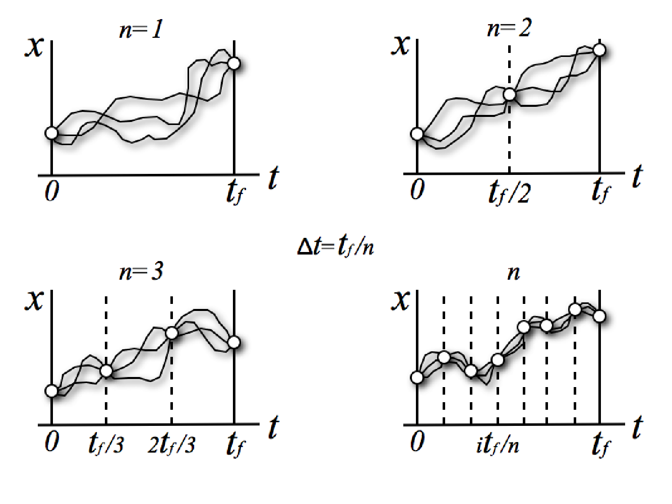
For simplicity we will consider that the coarse graining is into equal divisions of the total time duration . Therefore, in this -slicing procedure, the full trajectory of the particle is not measured but only its position after time intervals of duration . See figure (1). The probability for a discretized path can be easily evaluated since the process is Markovian and Gaussian. Let us denote by the conditional probability for jumping from a point at time to a point at time , and let be the initial equilibrium distribution. The probability of the -sliced discretized path is then given by
| (20) |
An analogous expression is valid for the backward path and probability, with superscript “tilde” again referring to time reversed excursion. The central quantity to evaluate is the following coarse-grained relative entropy (multiplied by , since we want to compare with the dissipated work, and having absorbed in its units):
| (21) |
The brackets refer to the average performed with the forward distribution .
The next step is to find the general expression for and . Since the Langevin equation that describes the dynamics is linear, the conditional probabilities are Gaussian distributions
| (22) |
and
| (23) |
From equation (18) (applied for final and initial times and , respectively, and with the appropriate initial condition) the conditional averages are found to be
| (24) |
and
| (25) |
where
| (26) |
Similarly, one can multiply the Langevin equation by the position and then take averages. This leads to the following equation for the variance :
| (27) |
which yields (conditional variances starting at zero value)
| (28) |
for both (forward and backward) cases.
In order to obtain , we insert the above conditional probability distributions in Eq. (21), work out the squares and arrange the averages. The final result can most revealingly be written in terms of the duration of the experiment and the final position . After some algebra, one finally gets
| (29) |
We also mention explicitly the results for and :
| (30) |
and
| (31) |
First note that in the limit one finds (cf. Eq. (19))
| (32) |
Hence the exact dissipation is, as anticipated, recovered in the limit of the continuous path description. Using the same procedure, one can show that this result remains valid for a general time dependent potential (see the Appendix).
We now turn to the main question of interest here. How is the convergence of to ? First, one can verify that, for any value of the system’s parameters, is always a lower bound for the total dissipation:
| (33) |
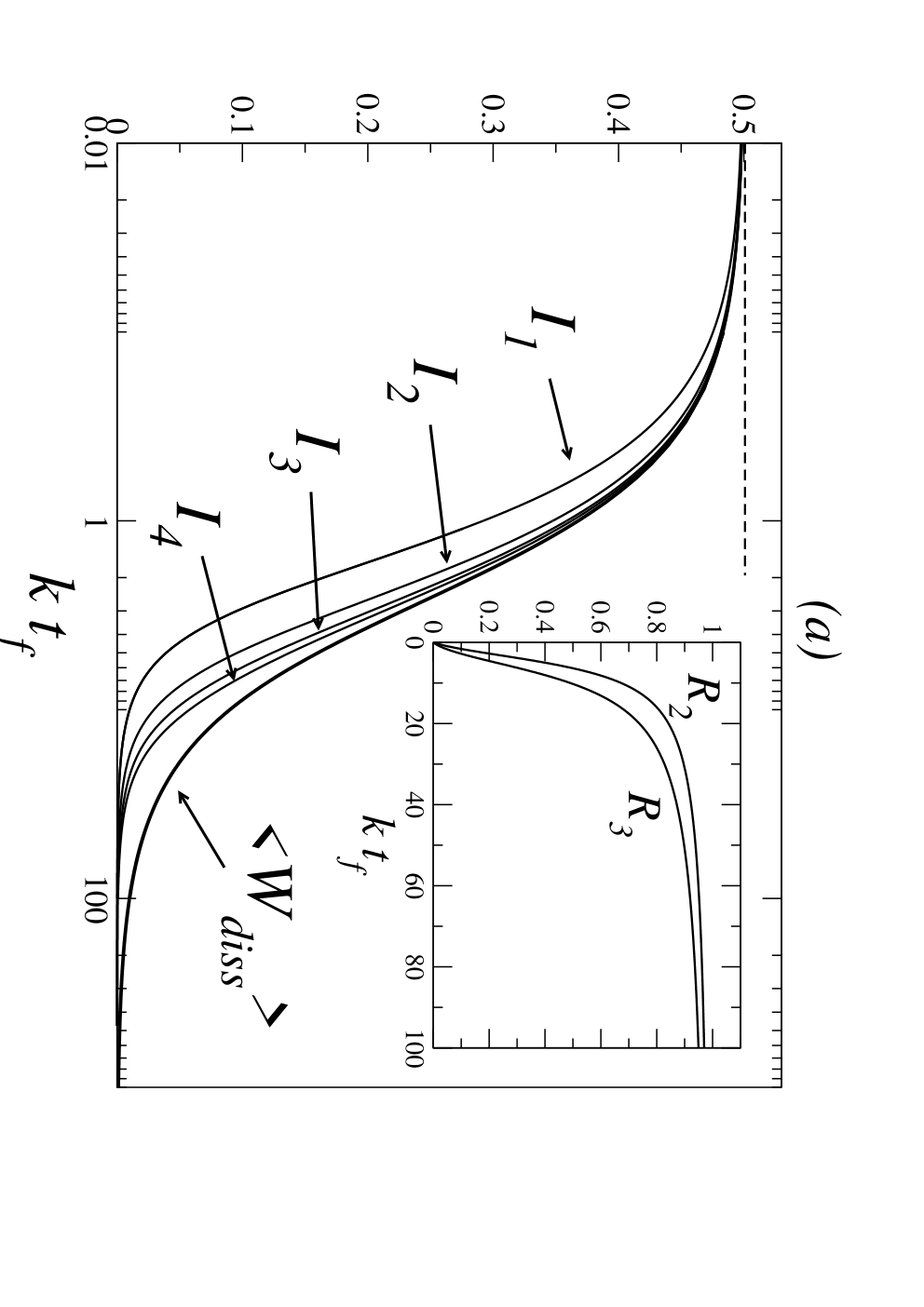
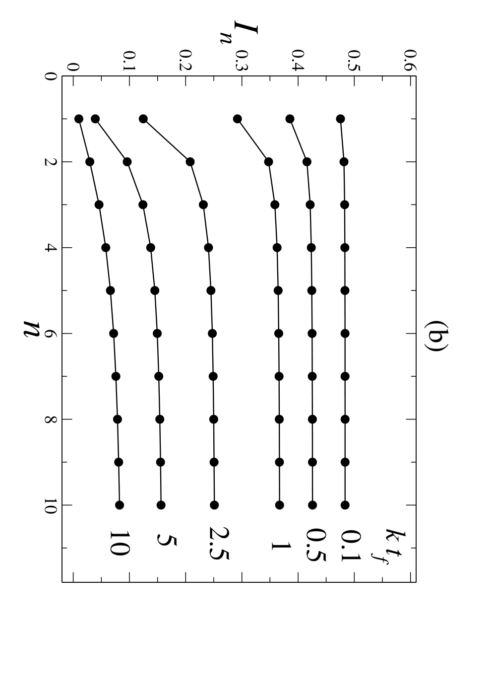
Next, as is apparent from the explicit result, the convergence of to depends only on the ratio of the time of the experiment over the relaxation time in the harmonic potential. In figure (2.a) we plot up to , as a function of . The convergence is surprisingly good. For example, for , the error in (single intermediate measurement point, plus the initial and the final points, which are always measured) is only a few percent. We also study in figure (2.b) the evolution of , for different values of , as the number of measured points increases. Note that the biggest jumps in occur from to , after which the bound quickly saturates and slowly approaches the total mean dissipated work.
In the limit or (very slow translation of the potential), one recovers the quasi-static result of zero dissipated work. Note however that the relative rate of convergence becomes quite bad in this limit (cf. inset in figure (2.a)). On the other hand, the fit is perfect in the limit of the irreversible quench, in which the potential is instantaneously switched to its new position. This corresponds to the limit or . One finds
| (34) |
The dissipated work is exactly equal to the average work done in instantaneously placing the particle in the shifted potential.
4 Underdamped Brownian particle: coarse graining in the space of variables
According to Eq. (1), the average dissipated work is obtained from a single time measurement of forward and backward statistics of the full system. Eq. (2) provides a complimentary result, since the measurement of some (e.g. heat bath) variables can be avoided and the average dissipated work is still obtained if the reduced set of stochastic variables are measured along the whole time track of the experiment. In the previous section, we discussed the effect of coarse graining in time for the measurement of the single relevant variable at hand, namely the position of the overdamped Brownian particle. In this section, we address the additional question about the role of specific variables (or degrees of freedom) in revealing the dissipation.
We naturally turn for the illustration of this point to underdamped Brownian particles in a harmonic potential since both position and momentum of the particle are relevant. Instead of considering a moving harmonic potential with fixed strength, we turn to another experimentally significant scenario of a non-moving harmonic potential undergoing an instantaneous quench, say at the initial time from a frequency to the frequency .
The point in phase space of all degrees of freedom, denoted previously by , and which includes all the bath variables, is supposed not to be accessible. As available statistical information we consider the probability distribution for position and momentum at a single arbitrary instant of time after the quench. Then, statistical information on this reduced set of variables at just one particular time must provide again lower bound for the dissipated work corresponding to such quench:
| (35) |
Below we will elucidate the effect of coarse graining implied in the punctual measurement in time (at time ) and, moreover, on a reduction in the number of variables (measuring only , only or both). Note that we are free to decide what we call the final time of the experiment, hence the choice of the measurement time after the quench is also completely free.
4.1 Mean dissipated work
The average work dissipated at the moment of the instantaneous quench can be evaluated as follows. The potential energy of the particle when at a position , is given by , where is the harmonic frequency, with and before and after the quench, respectively. The probability distribution of the position at the moment of the quench is given by (as before, Boltzmann’s constant is absorbed in the temperature for simplicity of notation). Here , the normalization constant, is the familiar partition function. Averaging with respect to this distribution (notation ), we conclude that the average work associated to the quench is given by . The corresponding change in free energy is found to be . Therefore, the total dissipation in the irreversible instantaneous quench reads
| (36) |
Note that the total dissipated work is always positive due to the irreversible nature of the process.
4.2 Probability density in forward and backward scenario
To obtain the bound from the coarse-grained relative entropy appearing in the r.h.s. of Eq. (35), we need to evaluate the probability distributions in forward and backward scenario. The derivation for the backward scenario is very simple. The system starts at canonical equilibrium with frequency , and the quench is performed at the end of the experiment ( in forward time, which is the final time in the reverse experiment). The particle is then at canonical equilibrium with respect to the frequency throughout the process, so that
| (37) |
Note that the distribution is even in , namely . Hence the distribution is Gaussian with the following moments:
| (38) |
One the other hand, in the forward scenario, the initial condition is canonical with respect to the initial frequency , . At the frequency is suddenly changed to and then kept constant along the whole process. Therefore, the evolution of the system in the forward process consists of a relaxation to the new equilibrium state, . We write the familiar equations of motion for an underdamped Brownian particle for times
| (39) | |||||
| (40) |
where is the friction coefficient, and is Gaussian white noise with strength determined by the fluctuation dissipation theorem, . The initial condition is stipulated by the fact that prior to the quench at , the system is at equilibrium in a harmonic potential with strength , i.e. it is bi-Gaussian with (compare with Eq. (4.2))
| (41) |
Since the Langevin equation is linear, the resulting time dependent probability distribution remains a Gaussian. Therefore, it is sufficient to evaluate the ensuing time evolution of first- and second-order moments. Since there is no shift in the center position of the harmonic potential, the average position and momentum stay equal to zero: . The second order moments on the other hand obey the following evolution equations which following directly from the equations (39) and (40):
| (42) |
These have to be solved with the above mentioned initial conditions. One finds:
| (43) |
| (44) |
| (45) |
where
| (46) |
Note the switch from a monotonously decay ( real) to an oscillatory one ( imaginary) of the above solutions for the moments as crosses the value from below.
4.3 Relative entropy
We are now in position to evaluate the relative entropy (or Kullback–Leibler distance) between and . The relative entropy between the forward and the backward distribution can be considered as a distance between and its final equilibrium state , only reached for . Since both densities are Gaussian (and the backward distribution is even in ), the following simple result is obtained:
| (47) |
where and are the covariance matrices of the forward and backward distributions, respectively
| (48) |
| (49) |
The above result can be further simplified to
| (50) |
From now on, subindices in refer to the variables of the probability distributions for which the relative entropy is evaluated. We also mention the results for the relative entropy of the probability distribution of only the position and momentum :
| (51) |
| (52) |
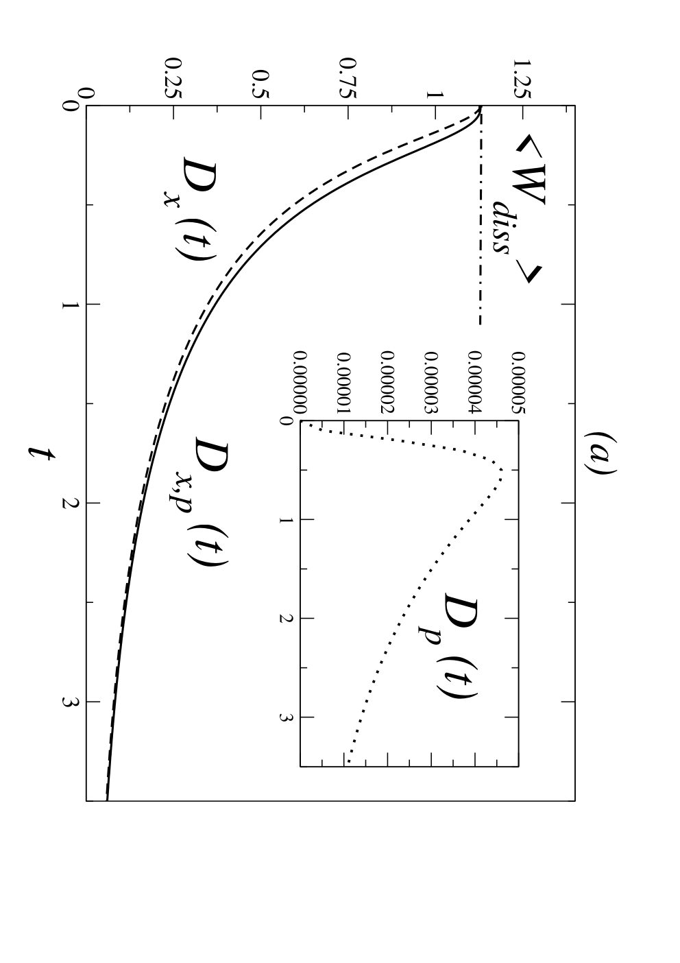
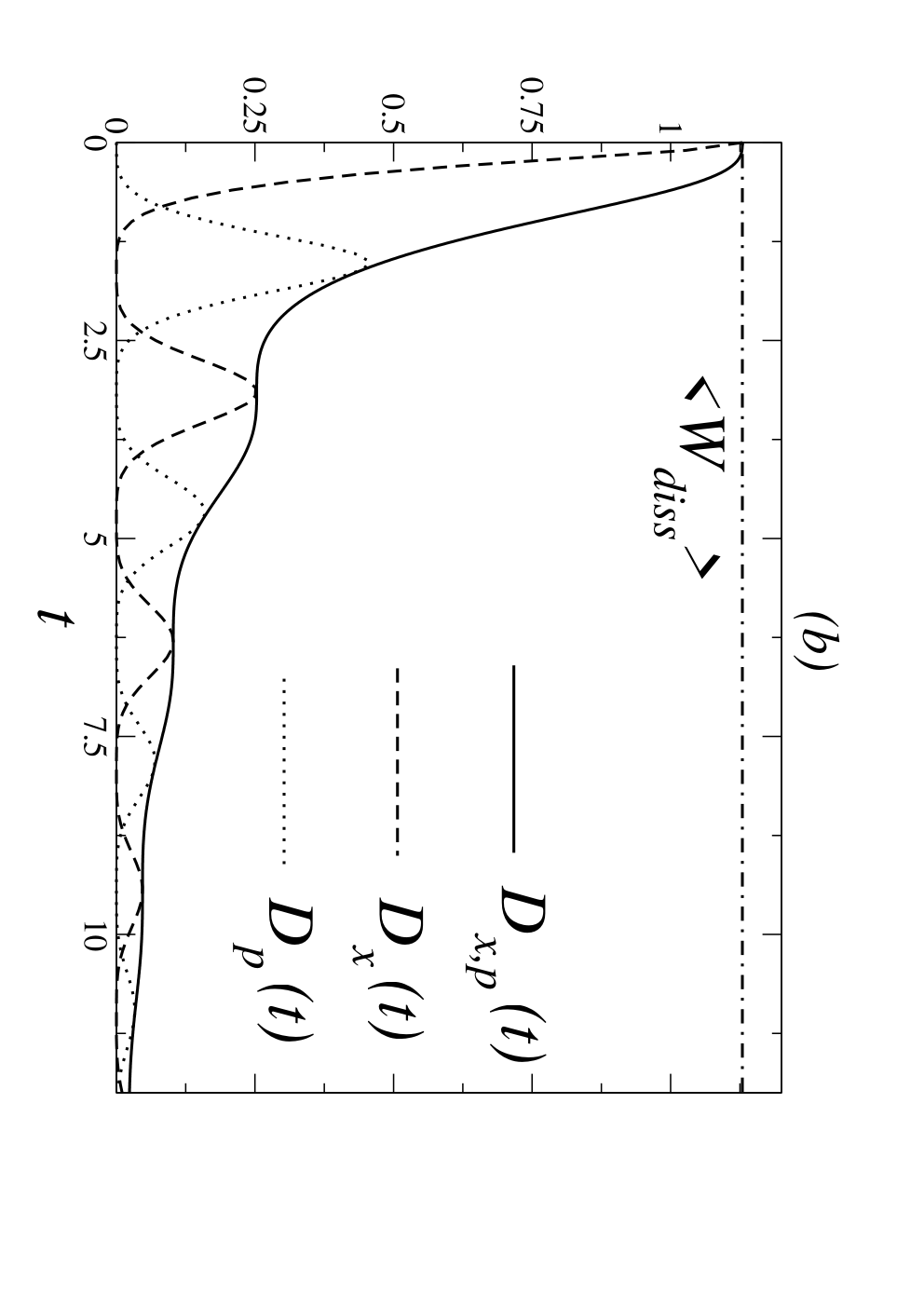
With these explicit results (depicted in figure 3), we can discuss how well the various relative entropies capture the dissipation. We first note that at the moment of the quench, full information on the dissipation is captured completely in the statistical information on the position variable (), while none is available from the momentum variable (). This is consistent with the observation that the position variable is the only variable which is out of equilibrium at this time.
Furthermore, it is known that the relative entropy between the probability distribution of a Markov process and its corresponding stationary state is a strictly decreasing function of time [20]. Hence, must be a decreasing function, as we have obtained in our calculation. However, the relative entropies when only one of the variables is taken into account exhibit a richer phenomenology.
The behavior is rather different in the weakly damped regime than in the strongly damped one. In the strongly damped case () the relative entropies and just decay monotonically with time, see figure (3.a). However, we obtain a non-monotonous behavior in the relative entropy of the momentum distribution. This can be explained as follows. The equilibrium distribution of the momentum does not depend on the frequency of the oscillator. Therefore, at the quench time, the forward and backward momentum distributions are identical. However, once the potential is quenched, the potential energy is not at equilibrium and as a consequence the kinetic energy momentum distribution will depart from equilibrium to relax back to the same distribution at a later time. As a consequence increases from , reaches a maximum and decays back to zero for long time, as can be seen in the inset of figure (3.a). The maximum is however very low, since damping is strong.
We can see a more pronounced and interesting effect in the underdamped case (). The main results are represented in figure (3.b). Note the oscillatory exchange of information on dissipation between the position and velocity variables and the decay of the total information contained in . In particular all the available information about the dissipation is periodically contained in one of the single variables, or , and it dies out (it gets lost in the bath degrees of freedom) as time evolves.
The peculiarities observed in the right figure (3.b) can be better understood by rewriting the relative entropy in (50) as follows:
| (53) |
where the correlation coefficient is given by
| (54) |
Since , we first note that the last term in the r.h.s of equation (53) is always positive, hence:
| (55) |
We conclude that, in the present case, the sum of information on the dissipation gathered separately from position and momentum is smaller than that from both variables taken together. The equality sign in (55) is realized when , or . Since the variables are Gaussian, the condition of zero correlation is tantamount to the independency of position and momentum. From the oscillating analogue of expression (45), one easily verifies that this occurs at specific times , where .
Another feature is that one of the variables, either or , loses all information on dissipation at another set of specific times. From equations (51) and (52) one finds that this occurs if or respectively. This is in agreement with the more general observation that the relative entropy of a specific degree of freedom is zero, when, at a given time, the detailed balance condition holds (i.e., when at that time the forward and backward distributions are equal).
We conclude that, on the whole, an intricate transfer of information on dissipation is taken place between position and momentum of the underdamped Brownian particle. At the same time, the information on the dissipated work is irreversibly lost by the punctual (one-time) relative entropy of and and transfered to the heat bath variables as time goes by.
5 Two coupled oscillators: flow of information on dissipation
To complete the picture, we next consider the case of a harmonically bound Brownian particle that is coupled, via a second Brownian particle, to the heat bath. The idea is that by monitoring this second particle, we are including some information on the heat bath (of which it is supposed to be part).
The Langevin equations of motion that describe the system read:
| (56) |
| (57) |
| (58) |
Again we consider the quench experiment. For times , the oscillator under consideration, oscillator , is initially at equilibrium with . At we perform an instantaneous quench switching so that for . Oscillator is kept throughout at the same frequency , while, on one hand, linearly coupled to oscillator with a strength and, on the other hand, immersed in the heat bath. The behavior of the first moments is trivial:
| (59) |
Furthermore, the probability distributions are all Gaussian so we only need to evaluate the second moments. Defining and , they obey the following set of evolution equations:
| (60) |
where the matrix is given by:
| (61) |
The system can be solved explicitly using the appropriate initial conditions. However, the analytic expressions are extremely lengthy. In what follows, we will illustrate the obtained behavior via appropriate figures.
5.1 Relative entropy
Since the joint distribution is Gaussian (and the backwards density even in ), the relative entropy involving all four variables and can be compactly expressed in terms of the covariance matrices and :
| (62) |
The latter are the following four-by-four symmetric matrices
| (63) |
Regarding the covariance matrix corresponding to the backwards excursion, we explicitly find
| (64) |
From the above results, we can derive the relative entropy of all available degrees of freedom of the system (both positions and , and momenta and ). While these are the pertinent variables to evaluate the dissipated work, when measured along the whole time track, a single time measurement as performed here again represents a coarse-graining. Only when performed at the moment of the quench does it contain full information. When considering times , information on the dissipation will flow and get irreversibly lost to the bath variables. This is similar to the situation discussed in the overdamped case
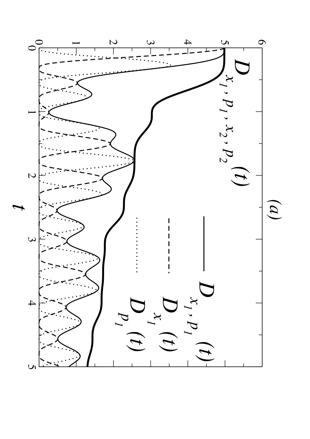
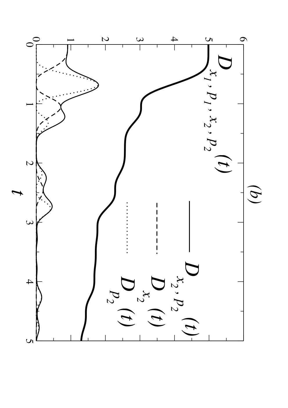
Similarly to the underdamped oscillator case, one can also explore the behavior of the relative entropies of all possible combinations of all 4 degrees of freedom , , and . Several of such combinations are plotted in figure 4. First note that, as explained before, the relative entropy of the whole system, , decays monotonically in time. Then, the relative entropy of oscillator , , is oscillating below the former. Both entropies for position and momentum alone, transfer information periodically and are modulated by . Note that the position of the first oscillator captures the whole dissipation at the moment of the quench,
| (65) |
The novelty in this case is that oscillator is not directly in contact with the heat bath, but rather to oscillator , whose relative entropies we now comment on. First, we see that the relative entropies are significantly smaller than those in oscillator . Oscillator 2 receives the information on the dissipated work from the quench only indirectly through its coupling to . Furthermore, while it “bounces” back some of this information to it also irreversibly loses information to the bath variables.
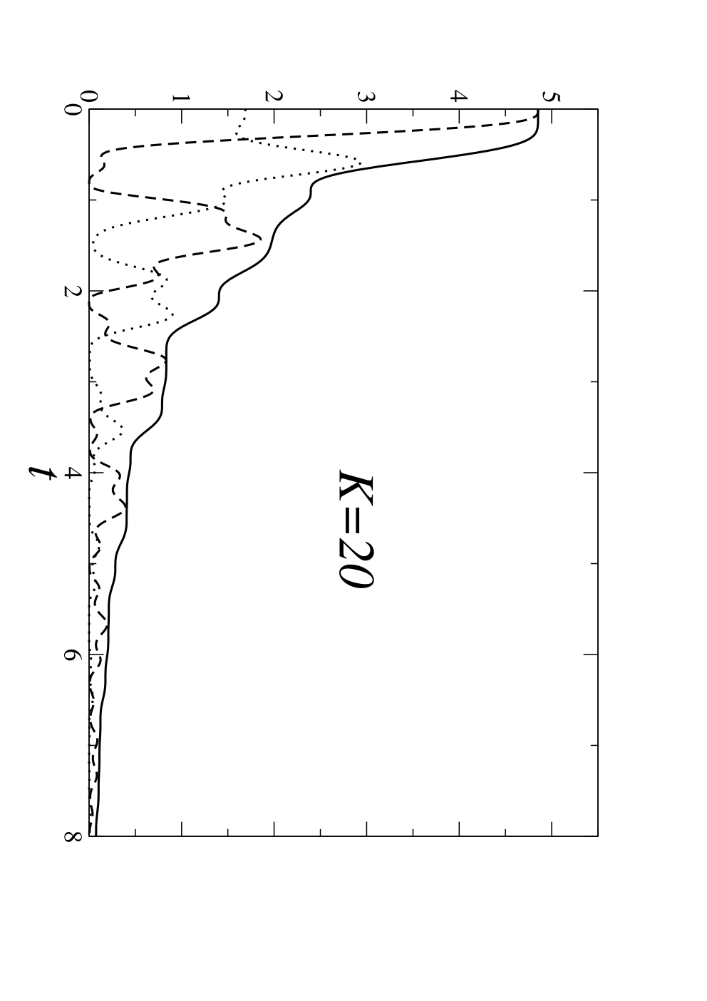
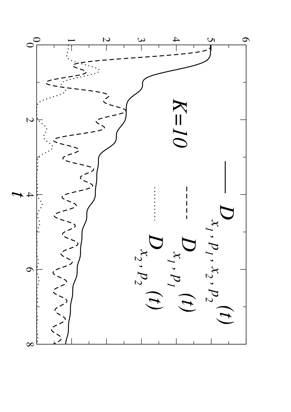
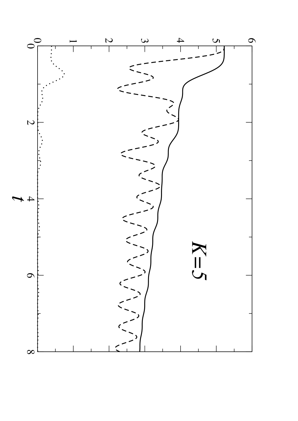
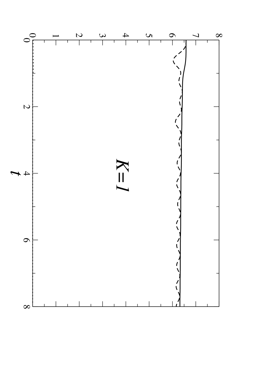
Regarding the plateau for the relative entropy appearing at short times in figure (4), one observes that most of the effect of the dissipative process still resides inside the system formed by the two particles. In fact, oscillator keeps much of this information while slowly transferring it to oscillator . Some of it can come back but a part of it is lost to the heat bath. This behavior is illustrated in figure (5) by varying the coupling constant that connects both oscillators. Note that for , the relative entropy of oscillator is almost zero but yet there is a considerable difference between and . Therefore, while oscillator is ”close to equilibrium”, its correlation with oscillator still carries relevant information on the irreversible quench.
6 Conclusions
We have derived a microscopically exact expression for the dissipative work along an arbitrary process starting in equilibrium for systems described by stochastic dynamics. As was anticipated in earlier work in the literature, we find that dissipation is proportional to the relative entropy between the probability distributions of forward and backward trajectories, respectively. In other words, dissipation is related to our ability to distinguish the arrow of time. Furthermore, the expression in terms of relative entropy gives rise to lower bounds if only partial information on the trajectories is available.
In combination with Crook’s theorem [24, 18], we have shown that a single functional of the path, namely the work itself, provides an exact and full assessment of dissipation. In other words, work ”exhausts” the arrow of time: if we know the statistical properties of the work done along the forward and the backward process, no further information can help us to better distinguish between the two.
We have discussed various scenarios to illustrate how dissipation can be bounded from below on the basis of reduced information. First, when the information about the continuous trajectory of the system is reduced to a finite number of measurements, our analysis has shown that the resulting relative entropy provides reasonably accurate bounds for the dissipation, even with only a small number of intermediate measurement points. This result could be specially useful in real experiments where trajectories are recorded at finite sampling rates. Second, we have analyzed the effect of considering a subset of variables instead of a detailed description of the system in a quench process. In this case, the time-arrow information, concentrated in the single position variable immediately after the quench, is subsequently transferred to the thermal bath and the other variables. Of special interest is the case of two oscillators, the first one undergoing a quench of its frequency and the second one in contact with a thermal bath. One would expect that the information contained in the first oscillator would be transferred to the second one before getting lost in the thermal bath. However, our analysis calls into question this naive picture, as we have shown that the oscillator coupled to the thermal bath is the first to thermalize. This result indicates that “reversibility”ââ is transferred from the thermal bath to the quench point, instead of “irreversibility” being transferred in the opposite direction. The generalization of our analysis to long chains of oscillators will help to further elucidate this issue.
Appendix
We studied the effect of coarse-graining in time for the harmonic potential. However, the same procedure can be applied for an arbitrary potential, at least in the limit of a infinitely large number of time measurements. Indeed the Gaussian ansatz remains valid for any potential for for short time increments, since the propagator of the Fokker-Planck equation is then always Gaussian [45]. Therefore, equations (22) and (23) are completely general in this case. The only difference is the expression for the first and second moments, but even this we know, since
| (66) |
On the whole, for small , the Fokker-Planck equation of such transition probabilities can be solved giving rise to [46]
| (67) |
Now we recall equation (21), and we find that the first term in the r.h.s. gives
| (68) |
where . After substitution of the conditional probabilities and some algebra, the second term in the r.h.s. of (21) yields to
| (69) |
where
| (70) |
| (71) |
Remember that this result is valid for small , or conversely, for big . In the limit of , we find to lowest order in that and , hence:
| (72) |
The last integral is the heat associated to a specific stochastic trajectory, cf. Eq. (15). Then, relations (21), (68), (69) and (72), together with the conservation of energy, imply that
| (73) |
This is a pedestrian path integral method to show that, for a general time dependent potential, the relative entropy of the distributions of the forward and backward paths (considering also their initial ensemble probabilities) is equal to the dissipated work.
References
References
- [1] Onsager L 1932 Phys. Rev. 37 405
- [2] Onsager L 1931 Phys. Rev. 38 2265
- [3] Prigogine I 1947 Etude Thermodynamique des Phénomènes Irréversibles (Desoer: Liège)
- [4] de Groot S R and Mazur P 1984 Non-Equilibrium Thermodynamics (Dover: New York)
- [5] Evans D J, Cohen E G D and Morriss G P 1993 Phys. Rev. Lett. 71 2401
- [6] Gallavotti G and Cohen E G D 1995 J. Stat. Phys. 80 931
- [7] Kurchan J 1998 J. Phys. A 31 3719
- [8] Lebowitz J L and Spohn H 1999 J. Stat. Phys. 95 333
- [9] Maes C 1999 J. Stat. Phys. 95 367
- [10] Bochkov G N and Kuzovlev Y E 1977 Zh. Eksp. Teor. Fiz. 72 238
- [11] Bochkov G N and Kuzovlev Y E 1977 Sov. Phys. JETP 45 125
- [12] Bochkov G N and Kuzovlev Y E 1981 Physica A 106 443
- [13] Bochkov G N and Kuzovlev Y E 1981 Physica A 106 480
- [14] Jarzynski C 1997 Phys. Rev. Lett. 78 2690
- [15] Jarzynski C 1997 Phys. Rev. E 56 5018
- [16] Crooks G E 1999 Phys. Rev. E 60 2721
- [17] Hatano T and Sasa S I 2001 Phys. Rev. Lett. 86 3463
- [18] Cleuren B, Van den Broeck C and Kawai R 2006 Phys. Rev. Lett. 96 050601
- [19] Kawai R, Parrondo J M R and Van den Broeck C 2007 Phys. Rev. Lett. 98 080602
- [20] Cover T M and Thomas J A 2006 Elements of Information Theory 2nd edition (Wiley, Hoboken: New Jersey)
- [21] Van Kampen N G 1992 Stochastic Processes in Physics and Chemistry (North Holland: Amsterdam)
- [22] Trepagnier E H, Jarzynski C, Ritort F, Crooks G E, Bustamante C J and Liphardt J 2005 Proc. Nat. Acad. Sci. 101 15038
- [23] Andrieux D, Gaspard P, Ciliberto S, Garnier N, Joubaud S and Petrosyan A 2007 Phys. Rev. Lett. 98 150601
- [24] Crooks G E 1998 J. Stat. Phys. 90 1481
- [25] Crooks G E 1999, Excursions in Statistical Dynamics, PhD thesis, University of Berkeley
- [26] Mackey M C 1989 Rev. Mod. Phys. 61 981
- [27] Vedral V 2002 Rev. Mod. Phys. 74 197
- [28] Jarzynski C 2006 Phys. Rev. E 73 046105
- [29] Luo Jiu-Li, Van den Broeck C and Nicolis G 1984 Z. Phys. B 56 165
- [30] Sekimoto K 1998 Prog. Theor. Phys. Suppl. 130 17
- [31] Kurchan J 1998 J. Phys. A 31 3719
- [32] Qian H 2001 Phys. Rev. E 63 042103
- [33] Maes C and Netocÿny K 2003 J. Stat. Phys. 110 269
- [34] Wu D and Kofke D A 2005 J. Chem. Phys. 123 054103
- [35] Seifert U 2005 Phys. Rev. Lett. 95 040602
- [36] Porporato A, Rigby J R and Daly E 2007 Phys. Rev. Lett. 98 094101
- [37] Gaspard P 2004 J. Stat. Phys. 117 599
- [38] Farago J 2002 J. Stat. Phys. 107 781, Farago J 2004 Physica A 331 69
- [39] van Zon R and Cohen E G D 2003 Phys. Rev. Lett. 91 110601
- [40] Blickle V, Speck T, Helden L, Seifert U and Bechinger C 2006 Phys. Rev. Lett. 96 070603
- [41] Gomez-Marin A and Sancho J M 2006 Phys. Rev. E 73 045101(R)
- [42] P. Visco 2006 J. Stat. Mech. P06006
- [43] Baiesi M, Jacobs T, Maes C and N.S. Skantzos, 2006 Phys. Rev. E 74 021111
- [44] F. Douarche, S. Joubaud, N.B. Garnier, A. Petrosyan, S. Ciliberto 2006 Phys. Rev. Lett. 97 140603
- [45] Risken H 1989 The Fokker-Planck equation: Methods of Solutions and Applications, 2nd edition (Springer-Verlag: Berlin)
- [46] Gardiner 1985 Handbook of Stochastic Methods (Springer-Verlag: Berlin)