CERN-PH-TH/2007-201 Topics on String PhenomenologyLectures given at Les Houches 2007 Summer School ‘String Theory and the Real World - From particle physics to astrophysics’, 2 - 27 July 2007

During the last few decades, physics beyond the Standard Model (SM) was guided from the problem of mass hierarchy. This can be formulated as the question of why gravity appears to us so weak compared to the other three known fundamental interactions corresponding to the electromagnetic, weak and strong nuclear forces. Indeed, gravitational interactions are suppressed by a very high energy scale, the Planck mass $M_{P}\sim 10^{19}$ GeV, associated to a length $l_{P}\sim 10^{-35}$ m, where they are expected to become important. In a quantum theory, the hierarchy implies a severe fine tuning of the fundamental parameters in more than 30 decimal places in order to keep the masses of elementary particles at their observed values. The reason is that quantum radiative corrections to all masses generated by the Higgs vacuum expectation value (VEV) are proportional to the ultraviolet cutoff which in the presence of gravity is fixed by the Planck mass. As a result, all masses are “attracted” to become about $10^{16}$ times heavier than their observed values.

Besides compositeness, there are three main ideas that have been proposed and studied extensively during the last years, corresponding to different approaches of dealing with the mass hierarchy problem. (1) Low energy supersymmetry with all superparticle masses in the TeV region. Indeed, in the limit of exact supersymmetry, quadratically divergent corrections to the Higgs self-energy are exactly cancelled, while in the softly broken case, they are cutoff by the supersymmetry breaking mass splittings. (2) TeV scale strings, in which quadratic divergences are cutoff by the string scale and low energy supersymmetry is not needed. (3) Split supersymmetry, where scalar masses are heavy while fermions (gauginos and higgsinos) are light. Thus, gauge coupling unification and dark matter candidate are preserved but the mass hierarchy should be stabilized by a different way and the low energy world appears to be fine-tuned. All these ideas are experimentally testable at high-energy particle colliders and in particular at LHC. Below, I discuss their implementation in string theory.

The appropriate and most convenient framework for low energy supersymmetry and grand unification is the perturbative heterotic string. Indeed, in this theory, gravity and gauge interactions have the same origin, as massless modes of the closed heterotic string, and they are unified at the string scale $M_{s}$. As a result, the Planck mass $M_{P}$ is predicted to be proportional to $M_{s}$:

$$M_{P}=M_{s}/g\,,$$

(1)

where $g$ is the gauge coupling. In the simplest constructions all gauge couplings are the same at the string scale, given by the four-dimensional (4d) string coupling, and thus no grand unified group is needed for unification. In our conventions $\alpha_{\rm GUT}=g^{2}\simeq 0.04$, leading to a discrepancy between the string and grand unification scale $M_{\rm GUT}$ by almost two orders of magnitude. Explaining this gap introduces in general new parameters or a new scale, and the predictive power is essentially lost. This is the main defect of this framework, which remains though an open and interesting possibility [1].

The other two ideas have both as natural framework of realization type I string theory with D-branes. Unlike in the heterotic string, gauge and gravitational interactions have now different origin. The latter are described again by closed strings, while the former emerge as excitations of open strings with endpoints confined on D-branes [2]. This leads to a braneworld description of our universe, which should be localized on a hypersurface, i.e. a membrane extended in $p$ spatial dimensions, called $p$-brane (see Fig. 1). Closed strings propagate in all nine dimensions of string theory: in those extended along the $p$-brane, called parallel, as well as in the transverse ones. On the contrary, open strings are attached on the $p$-brane.

Obviously, our $p$-brane world must have at least the three known dimensions of space. But it may contain more: the extra $d_{\parallel}=p-3$ parallel dimensions must have a finite size, in order to be unobservable at present energies, and can be as large as TeV${}^{-1}\sim 10^{-18}$ m [3]. On the other hand, transverse dimensions interact with us only gravitationally and experimental bounds are much weaker: their size should be less than about 0.1 mm [4]. In the following, I review the main properties and experimental signatures of low string scale models [5, 6].

These lectures have two parts. In the first part, contained in sections 2 to 6, I describe the implementation, the properties and the main phyical properties of low scale string theories. In the second part, contained in the following sections, starting from section 7, I discuss a simple framework of toroidal type I string compactifications with in general high string scale, in the presence of magnetized branes, that can be used for moduli stabilization, model building and supersymmetry breaking.

In type I theory, the different origin of gauge and gravitational interactions implies that the relation between the Planck and string scales is not linear as (1) of the heterotic string. The requirement that string theory should be weakly coupled, constrain the size of all parallel dimensions to be of order of the string length, while transverse dimensions remain unrestricted. Assuming an isotropic transverse space of $n=9-p$ compact dimensions of common radius $R_{\perp}$, one finds:

$$M_{P}^{2}=\frac{1}{g^{4}}M_{s}^{2+n}R_{\perp}^{n}\ ,\qquad g_{s}\simeq g^{2}\,.$$

(2)

where $g_{s}$ is the string coupling. It follows that the type I string scale can be chosen hierarchically smaller than the Planck mass [7, 5] at the expense of introducing extra large transverse dimensions felt only by gravity, while keeping the string coupling small [5]. The weakness of 4d gravity compared to gauge interactions (ratio $M_{W}/M_{P}$) is then attributed to the largeness of the transverse space $R_{\perp}$ compared to the string length $l_{s}=M_{s}^{-1}$.

An important property of these models is that gravity becomes effectively $(4+n)$-dimensional with a strength comparable to those of gauge interactions at the string scale. The first relation of Eq. (2) can be understood as a consequence of the $(4+n)$-dimensional Gauss law for gravity, with

$$M_{*}^{(4+n)}=M_{s}^{2+n}/g^{4}$$

(3)

the effective scale of gravity in $4+n$ dimensions. Taking $M_{s}\simeq 1$ TeV, one finds a size for the extra dimensions $R_{\perp}$ varying from $10^{8}$ km, .1 mm, down to a Fermi for $n=1,2$, or 6 large dimensions, respectively. This shows that while $n=1$ is excluded, $n\geq 2$ is allowed by present experimental bounds on gravitational forces [4, 8]. Thus, in these models, gravity appears to us very weak at macroscopic scales because its intensity is spread in the “hidden” extra dimensions. At distances shorter than $R_{\perp}$, it should deviate from Newton’s law, which may be possible to explore in laboratory experiments (see Fig. 2).

The main experimental implications of TeV scale strings in particle accelerators are of three types, in correspondence with the three different sectors that are generally present: (i) new compactified parallel dimensions, (ii) new extra large transverse dimensions and low scale quantum gravity, and (iii) genuine string and quantum gravity effects. On the other hand, there exist interesting implications in non accelerator table-top experiments due to the exchange of gravitons or other possible states living in the bulk.

Non-supersymmetric TeV strings offer also a framework to realize gauge symmetry breaking radiatively. Indeed, from the effective field theory point of view, one expects quadratically divergent one-loop contributions to the masses of scalar fields. The divergences are cut off by $M_{s}$ and if the corrections are negative, they can induce electroweak symmetry breaking and explain the mild hierarchy between the weak and a string scale at a few TeV, in terms of a loop factor [35]. More precisely, in the minimal case of one Higgs doublet $H$, the scalar potential is:

$$V=\lambda(H^{\dagger}H)^{2}+\mu^{2}(H^{\dagger}H)\,,$$

(13)

where $\lambda$ arises at tree-level. Moreover, in any model where the Higgs field comes from an open string with both ends fixed on the same brane stack, it is given by an appropriate truncation of a supersymmetric theory. Within the minimal spectrum of the SM, $\lambda=(g_{2}^{2}+g^{\prime 2})/8$, with $g_{2}$ and $g^{\prime}$ the $SU(2)$ and $U(1)_{Y}$ gauge couplings. On the other hand, $\mu^{2}$ is generated at one loop:

$$\mu^{2}=-\varepsilon^{2}\,g^{2}\,M_{s}^{2}\,,$$

(14)

where $\varepsilon$ is a loop factor that can be estimated from a toy model computation and varies in the region $\epsilon\sim 10^{-1}-10^{-3}$.

Indeed, consider for illustration a simple case where the whole one-loop effective potential of a scalar field can be computed. We assume for instance one extra dimension compactified on a circle of radius $R>1$ (in string units). An interesting situation is provided by a class of models where a non-vanishing VEV for a scalar (Higgs) field $\phi$ results in shifting the mass of each KK excitation by a constant $a(\phi)$:

$$M^{2}_{m}=\left(\frac{m+a(\phi)}{R}\right)^{2}\,,$$

(15)

with $m$ the KK integer momentum number. Such mass shifts arise for instance in the presence of a Wilson line, $a=q\oint\frac{dy}{2\pi}gA$, where $A$ is the internal component of a gauge field with gauge coupling $g$, and $q$ is the charge of a given state under the corresponding generator. A straightforward computation shows that the $\phi$-dependent part of the one-loop effective potential is given by [36]:

$$V_{eff}=-Tr(-)^{F}\,\frac{R}{32\,\pi^{3/2}}\,\,\sum_{n}e^{2\pi ina}\,\,\int_{0}^{\infty}dl\,\,l^{3/2}f_{s}(l)\,\,e^{-\pi^{2}n^{2}R^{2}l}$$

(16)

where $F=0,1$ for bosons and fermions, respectively. We have included a regulating function $f_{s}(l)$ which contains for example the effects of string oscillators. To understand its role we will consider the two limits $R>>1$ and $R<<1$. In the first case only the $l\rightarrow 0$ region contributes to the integral. This means that the effective potential receives sizable contributions only from the infrared (field theory) degrees of freedom. In this limit we would have $f_{s}(l)\rightarrow 1$. For example, in the string model considered in [35]:

$$f_{s}(l)=\left[\frac{1}{4l}\frac{\theta_{2}}{\eta^{3}}(il+{\frac{1}{2}})\right]^{4}\rightarrow 1\qquad{\rm for}\qquad l\rightarrow 0,$$

(17)

and the field theory result is finite and can be explicitly computed. As a result of the Taylor expansion around $a=0$, we are able to extract the one-loop contribution to the coefficient of the term of the potential quadratic in the Higgs field. It is given by a loop factor times the compactification scale [36]. One thus obtains $\mu^{2}\sim g^{2}/R^{2}$ up to a proportionality constant which is calculable in the effective field theory. On the other hand, if we consider $R\rightarrow 0$, which by $T$-duality corresponds to taking the extra dimension as transverse and very large, the one-loop effective potential receives contributions from the whole tower of string oscillators as appearing in $f_{s}(l)$, leading to squared masses given by a loop factor times $M_{s}^{2}$, according to eq. (14).

More precisely, from the expression (16), one finds:

$$\varepsilon^{2}(R)={1\over 2\pi^{2}}\int_{0}^{\infty}\frac{dl}{\left(2\,l\right)^{5/2}}{\theta_{2}^{4}\over 4\eta^{12}}\left(il+{1\over 2}\right)R^{3}\sum_{n}n^{2}e^{-2\pi n^{2}R^{2}l}\ ,$$

(18)

which is plotted in Fig. 9.

For the asymptotic value $R\to 0$ (corresponding upon T-duality to a large transverse dimension of radius $1/R$), $\varepsilon(0)\simeq 0.14$, and the effective cut-off for the mass term is $M_{s}$, as can be seen from Eq. (14). At large $R$, $\mu^{2}(R)$ falls off as $1/R^{2}$, which is the effective cut-off in the limit $R\to\infty$, as we argued above, in agreement with field theory results in the presence of a compactified extra dimension [37, 26]. In fact, in the limit $R\to\infty$, an analytic approximation to $\varepsilon(R)$ gives:

$$\varepsilon(R)\simeq\frac{\varepsilon_{\infty}}{M_{s}\,R}\,,\qquad\qquad\varepsilon_{\infty}^{2}=\frac{3\,\zeta(5)}{4\,\pi^{4}}\simeq 0.008\,.$$

(19)

The potential (13) has the usual minimum, given by the VEV of the neutral component of the Higgs doublet $v=\sqrt{-\mu^{2}/\lambda}$. Using the relation of $v$ with the $Z$ gauge boson mass, $M_{Z}^{2}=(g_{2}^{2}+g^{\prime 2})v^{2}/4$, and the expression of the quartic coupling $\lambda$, one obtains for the Higgs mass a prediction which is the Minimal Supersymmetric Standard Model (MSSM) value for $\tan\beta\to\infty$ and $m_{A}\to\infty$: $m_{H}=M_{Z}$. The tree level Higgs mass is known to receive important radiative corrections from the top-quark sector and rises to values around 120 GeV. Furthermore, from (14), one can compute $M_{s}$ in terms of the Higgs mass $m_{H}^{2}=-2\mu^{2}$:

$$M_{s}=\frac{m_{H}}{\sqrt{2}\,g\varepsilon}\,,$$

(20)

yielding naturally values in the TeV range.

The gauge group closest to the Standard Model one can easily obtain with D-branes is $U(3)\times U(2)\times U(1)$. The first factor arises from three coincident “color” D-branes. An open string with one end on them is a triplet under $SU(3)$ and carries the same $U(1)$ charge for all three components. Thus, the $U(1)$ factor of $U(3)$ has to be identified with gauged baryon number. Similarly, $U(2)$ arises from two coincident “weak” D-branes and the corresponding abelian factor is identified with gauged weak-doublet number. Finally, an extra $U(1)$ D-brane is necessary in order to accommodate the Standard Model without breaking the baryon number [38]. In principle this $U(1)$ brane can be chosen to be independent of the other two collections with its own gauge coupling. To improve the predictability of the model, we choose to put it on top of either the color or the weak D-branes [39]. In either case, the model has two independent gauge couplings $g_{3}$ and $g_{2}$ corresponding, respectively, to the gauge groups $U(3)$ and $U(2)$. The $U(1)$ gauge coupling $g_{1}$ is equal to either $g_{3}$ or $g_{2}$.

Let us denote by $Q_{3}$, $Q_{2}$ and $Q_{1}$ the three $U(1)$ charges of $U(3)\times U(2)\times U(1)$, in a self explanatory notation. Under $SU(3)\times SU(2)\times U(1)_{3}\times U(1)_{2}\times U(1)_{1}$, the members of a family of quarks and leptons have the following quantum numbers:

		$\displaystyle Q$	$\displaystyle({\bf 3},{\bf 2};1,w,0)_{1/6}$		(21)
		$\displaystyle u^{c}$	$\displaystyle({\bf\bar{3}},{\bf 1};-1,0,x)_{-2/3}$
		$\displaystyle d^{c}$	$\displaystyle({\bf\bar{3}},{\bf 1};-1,0,y)_{1/3}$
		$\displaystyle L$	$\displaystyle({\bf 1},{\bf 2};0,1,z)_{-1/2}$
		$\displaystyle l^{c}$	$\displaystyle({\bf 1},{\bf 1};0,0,1)_{1}$

The values of the $U(1)$ charges $x,y,z,w$ will be fixed below so that they lead to the right hypercharges, shown for completeness as subscripts.

It turns out that there are two possible ways of embedding the Standard Model particle spectrum on these stacks of branes [38], which are shown pictorially in Fig. 10.

The quark doublet $Q$ corresponds necessarily to a massless excitation of an open string with its two ends on the two different collections of branes (color and weak). As seen from the figure, a fourth brane stack is needed for a complete embedding, which is chosen to be a $U(1)_{b}$ extended in the bulk. This is welcome since one can accommodate right handed neutrinos as open string states on the bulk with sufficiently small Yukawa couplings suppressed by the large volume of the bulk [40]. The two models are obtained by an exchange of the up and down antiquarks, $u^{c}$ and $d^{c}$, which correspond to open strings with one end on the color branes and the other either on the $U(1)$ brane, or on the $U(1)_{b}$ in the bulk. The lepton doublet $L$ arises from an open string stretched between the weak branes and $U(1)_{b}$, while the antilepton $l^{c}$ corresponds to a string with one end on the $U(1)$ brane and the other in the bulk. For completeness, we also show the two possible Higgs states $H_{u}$ and $H_{d}$ that are both necessary in order to give tree-level masses to all quarks and leptons of the heaviest generation.

We now consider type I string theory, or equivalently type IIB with orientifold 9-planes and D9-branes [2]. Upon compactification in four dimensions on a Calabi-Yau manifold, one gets ${\cal N}=2$ supersymmetry in the bulk and ${\cal N}=1$ on the branes. We then turn on internal magnetic fields [43, 44], which, in the T-dual picture, amounts to intersecting branes [45, 46]. For generic angles, or equivalently for arbitrary magnetic fields, supersymmetry is spontaneously broken and described by effective D-terms in the four-dimensional (4d) theory [43]. In the weak field limit, $|H|\alpha^{\prime}<1$ with $\alpha^{\prime}$ the string Regge slope, the resulting mass shifts are given by:

$$\delta M^{2}=(2k+1)|qH|+2qH\Sigma\quad;\quad k=0,1,2,\dots\,,$$

(28)

where $H$ is the magnetic field of an abelian gauge symmetry, corresponding to a Cartan generator of the higher dimensional gauge group, on a non-contractible 2-cycle of the internal manifold. $\Sigma$ is the corresponding projection of the spin operator, $k$ is the Landau level and $q=q_{L}+q_{R}$ is the charge of the state, given by the sum of the left and right charges of the endpoints of the associated open string. We recall that the exact string mass formula has the same form as (28) with $qH$ replaced by:

$$qH\longrightarrow\theta_{L}+\theta_{R}\qquad;\qquad\theta_{L,R}=\arctan(q_{L,R}H\alpha^{\prime})\,.$$

(29)

Obviously, the field theory expression (28) is reproduced in the weak field limit.

The Gauss law for the magnetic flux implies that the field $H$ is quantized in terms of the area of the corresponding 2-cycle $A$:

$$H={m\over nA}\,,$$

(30)

where the integers $m,n$ correspond to the respective magnetic and electric charges; $m$ is the quantized flux and $n$ is the wrapping number of the higher dimensional brane around the corresponding internal 2-cycle. In the T-dual representation, associated to the inversion of the compactification radius along one of the two directions of the 2-cycle, $m$ and $n$ become the wrapping numbers around these two directions.

For simplicity, we consider first the case where the internal manifold is a product of three factorized tori $\prod_{i=1}^{3}T^{2}_{(i)}$. Then, the mass formula (28) becomes:

$$\delta M^{2}=\sum_{i}(2k_{i}+1)|qH_{i}|+2qH_{i}\Sigma_{i}\,,$$

(31)

where $\Sigma_{i}$ is the projection of the internal helicity along the $i$-th plane. For a ten-dimensional (10d) spinor, its eigenvalues are $\Sigma_{i}=\pm 1/2$, while for a 10d vector $\Sigma_{i}=\pm 1$ in one of the planes $i=i_{0}$ and zero in the other two $(i\neq i_{0})$. Thus, charged higher dimensional scalars become massive, fermions lead to chiral 4d zero modes if all $H_{i}\neq 0$, while the lightest scalars coming from 10d vectors have masses

$$M_{0}^{2}=\left\{\begin{matrix}|qH_{1}|+|qH_{2}|-|qH_{3}|\cr|qH_{1}|-|qH_{2}|+|qH_{3}|\cr-|qH_{1}|+|qH_{2}|+|qH_{3}|\cr\end{matrix}\,.\right.$$

(32)

Note that all of them can be made positive definite, avoiding the Nielsen-Olesen instability, if all $H_{i}\neq 0$. Moreover, one can easily show that if a scalar mass vanishes, some supersymmetry remains unbroken [44, 45].

We turn on now several abelian magnetic fields $H_{I}^{a}$ of different Cartan generators $U(1)_{a}$, so that the gauge group is a product of unitary factors $\prod_{a}U(N_{a})$ with $U(N_{a})=SU(N_{a})\times U(1)_{a}$. In an appropriate T-dual representation, it amounts to consider several stacks of D6-branes intersecting in the three internal tori at angles. An open string with one end on the $a$-th stack has charge $\pm 1$ under the $U(1)_{a}$, depending on its orientation, and is neutral with respect to all others.

In this section, we perform a general study of SM embedding in three brane stacks with gauge group $U(3)\times U(2)\times U(1)$ [47], and present an explicit example having realistic particle content and satisfying gauge coupling unification [48]. We consider in general non oriented strings because of the presence of the orientifold plane that gives rise mirror branes with opposite magnetic fluxes $m\to-m$ in eq. (30). An open string stretched between a brane stack $U(N)$ and its mirror transforms in the symmetric or antisymmetric representation, while the multiplicity of chiral fermions is given by their intersection number.

The quark and lepton doublets ($Q$ and $L$) correspond to open strings stretched between the weak and the color or $U(1)$ branes, respectively. On the other hand, the $u^{c}$ and $d^{c}$ antiquarks can come from strings that are either stretched between the color and $U(1)$ branes, or that have both ends on the color branes (stretched between the brane stack and its orientifold image) and transform in the antisymmetric representation of $U(3)$ (which is an anti-triplet). There are therefore three possible models, depending on whether it is the $u^{c}$ (model A), or the $d^{c}$ (model B), or none of them (model C), the state coming from the antisymmetric representation of color branes. It follows that the antilepton $l^{c}$ comes in a similar way from open strings with both ends either on the weak brane stack and transforming in the antisymmetric representation of $U(2)$ which is an $SU(2)$ singlet (in model A), or on the abelian brane and transforming in the “symmetric” representation of $U(1)$ (in models B and C). The three models are presented pictorially in Fig. 12

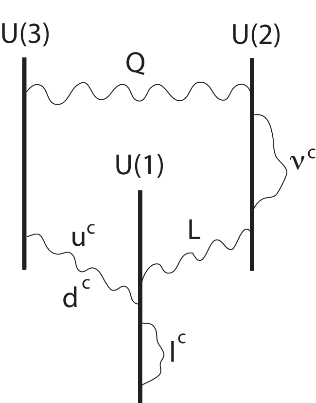
Thus, the members of a family of quarks and leptons have the following quantum numbers:

			$\displaystyle{\rm Model\ A}\qquad\qquad\quad\quad{\rm Model\ B}\qquad\qquad\quad\ {\rm Model\ C}$
	$\displaystyle\!\!\!\!\!\!\!\!Q$		$\displaystyle({\bf 3},{\bf 2};1,1,0)_{1/6}\quad\quad\quad\ ({\bf 3},{\bf 2};1,\varepsilon_{Q},0)_{1/6}\qquad\,({\bf 3},{\bf 2};1,\varepsilon_{Q},0)_{1/6}$
	$\displaystyle\!\!\!\!\!\!\!\!u^{c}$		$\displaystyle(\bar{\bf 3},{\bf 1};2,0,0)_{-2/3}\quad\quad\ \ \,(\bar{\bf 3},{\bf 1};-1,0,1)_{-2/3}\quad\ (\bar{\bf 3},{\bf 1};-1,0,1)_{-2/3}$
	$\displaystyle\!\!\!\!\!\!\!\!d^{c}$		$\displaystyle(\bar{\bf 3},{\bf 1};-1,0,\varepsilon_{d})_{1/3}\qquad\,(\bar{\bf 3},{\bf 1};2,0,0)_{1/3}\qquad\ \ \,(\bar{\bf 3},{\bf 1};-1,0,-1)_{1/3}$		(33)
	$\displaystyle\!\!\!\!\!\!\!\!L$		$\displaystyle({\bf 1},{\bf 2};0,-1,\varepsilon_{L})_{-1/2}\quad\ \,({\bf 1},{\bf 2};0,\varepsilon_{L},1)_{-1/2}\quad\ \ \,({\bf 1},{\bf 2};0,\varepsilon_{L},1)_{-1/2}$
	$\displaystyle\!\!\!\!\!\!\!\!l^{c}$		$\displaystyle({\bf 1},{\bf 1};0,2,0)_{1}\qquad\quad\quad\,({\bf 1},{\bf 1};0,0,-2)_{1}\qquad\ \ ({\bf 1},{\bf 1};0,0,-2)_{1}$
	$\displaystyle\!\!\!\!\!\!\!\!\nu^{c}$		$\displaystyle({\bf 1},{\bf 1};0,0,2\varepsilon_{\nu})_{0}\qquad\quad\ ({\bf 1},{\bf 1};0,2\varepsilon_{\nu},0)_{0}\qquad\ \,({\bf 1},{\bf 1};0,2\varepsilon_{\nu},0)_{0}$

where the last three digits after the semi-column in the brackets are the charges under the three abelian factors $U(1)_{3}\times U(1)_{2}\times U(1)$, that we will call $Q_{3}$, $Q_{2}$ and $Q_{1}$ in the following, while the subscripts denote the corresponding hypercharges. The various sign ambiguities $\varepsilon_{i}=\pm 1$ are due to the fact that the corresponding abelian factor does not participate in the hypercharge combination (see below). In the last lines, we also give the quantum numbers of a possible right-handed neutrino in each of the three models. These are in fact all possible ways of embedding the SM spectrum in three sets of branes.

The hypercharge combination is:

	$\displaystyle{\rm Model\ A}\quad\$	$\displaystyle:$	$\displaystyle\quad Y=-{1\over 3}Q_{3}+{1\over 2}Q_{2}$		(34)
	$\displaystyle{\rm Model\ B,C}$	$\displaystyle:$	$\displaystyle\quad Y=\ \ \,{1\over 6}Q_{3}-{1\over 2}Q_{1}$

leading to the following expressions for the weak angle:

	$\displaystyle{\rm Model\ A}$	$\displaystyle:$	$\displaystyle\sin^{2}\theta_{W}={1\over 2+2\alpha_{2}/3\alpha_{3}}={3\over 8}\,{\bigg|}_{\alpha_{{}_{2}}=\alpha_{{}_{3}}}$		(35)
	$\displaystyle{\rm Model\ B,C}$	$\displaystyle:$	$\displaystyle\sin^{2}\theta_{W}={1\over 1+\alpha_{2}/2\alpha_{1}+\alpha_{2}/6\alpha_{3}}$
			$\displaystyle\qquad\quad\ ={6\over 7+3\alpha_{2}/\alpha_{1}}\,{\bigg|}_{\alpha_{{}_{2}}=\alpha_{{}_{3}}}$

In the second part of the above equalities, we used the unification relation $\alpha_{2}=\alpha_{3}$, that can be imposed if for instance $U(3)$ and $U(2)$ branes are coincident, leading to a $U(5)$ unified group. Alternatively, this condition can be generally imposed under mild assumptions [48]. It follows that model A admits natural gauge coupling unification of strong and weak interactions, and predicts the correct value for $\sin^{2}\theta_{W}=3/8$ at the unification scale $M_{\rm GUT}$. On the other hand, model B corresponds to the flipped $SU(5)$ where the role of $u^{c}$ and $d^{c}$ is interchanged together with $l^{c}$ and $\nu^{c}$ between the ${\bf 10}$ and ${\bf\bar{5}}$ representations [49].

Besides the hypercharge combination, there are two additional $U(1)$’s. It is easy to check that one of the two can be identified with $B-L$. For instance, in model A choosing the signs $\varepsilon_{d}=\varepsilon_{L}=-\varepsilon_{\nu}=-\varepsilon_{H}=\varepsilon_{H^{\prime}}$, it is given by:

$$B-L=-{1\over 6}Q_{3}+{1\over 2}Q_{2}-{\varepsilon_{d}\over 2}Q_{1}\,.$$

(36)

Finally, the above spectrum can be easily implemented with a Higgs sector, since the Higgs field $H$ has the same quantum numbers as the lepton doublet or its complex conjugate.

Internal magnetic fluxes provide a new calculable method of moduli stabilization in four-dimensional (4d) type I string compactifications [50, 51, 52]. In fact, moduli stabilization in the presence of 3-form closed string fluxes led to significance progress over the last years [53, 54] but presents some drawbacks: (i) it has no exact string description and thus relies mainly on the low energy supergravity approximpation; (ii) in the generic case, it can fix only the complex structure and the dilaton [55], while for the Kähler class non-perturbative effects have to be used [54]. On the other hand, constant internal magnetic fields can stabilize mainly Kähler moduli [56, 50] and are thus complementary to 3-form closed string fluxes. Moreover, they can also be used in simple toroidal compactifications, stabilizing all geometric moduli in a supersymmetric vacuum using only magnetized $D9$-branes that have an exact perturbative string description [57, 43]. They have also a natural implementation in intersecting D-brane models.

Here, we make use of the conventions given in Appendix A of Ref. [51], for the parametrization of the torus $T^{6}$, as well as for the general definitions of the Kähler and complex structure moduli. In particular, the coordinates of three factorized tori: $(T^{2})^{3}\in T^{6}$ are given by $x_{i},y_{i}$ $i=1,2,3$ with periodicities: $x^{i}=x^{i}+1$, $y^{i}\equiv y^{i}+1$, and a volume normalization:

$$\int dx_{1}\wedge dy_{1}\wedge dx_{2}\wedge dy_{2}\wedge dx_{3}\wedge dy_{3}=1\,.$$

(37)

The 36 moduli of $T^{6}$ correspond to 21 independent deformations of the internal metric and 15 deformations of the two-index antisymmetric tensor $C_{2}$ from the RR closed string sector. They form nine complex parameters of Kähler class and nine of complex structure. Indeed, the geometric moduli decompose in a complex structure variation which is parametrized by the matrix $\tau_{ij}$ entering in the definition of the complex coordinates

$$z_{i}=x_{i}+\tau_{ij}y^{j}\,,$$

(38)

and in the Kähler variation of the mixed part of the metric described by the real $(1,1)$-form $J=i\delta g_{i\bar{j}}dz^{i}\wedge d\bar{z}^{j}$. The later is complexified with the corresponding RR two-form deformation.

References

- [1] Fore a review, see e.g. K. R. Dienes, Phys. Rept. 287 (1997) 447 [arXiv:hep-th/9602045]; and references therein.
- [2] C. Angelantonj and A. Sagnotti, Phys. Rept. 371 (2002) 1 [Erratum-ibid. 376 (2003) 339] [arXiv:hep-th/0204089].
- [3] I. Antoniadis, Phys. Lett. B 246 (1990) 377.
- [4] D. J. Kapner, T. S. Cook, E. G. Adelberger, J. H. Gundlach, B. R. Heckel, C. D. Hoyle and H. E. Swanson, Phys. Rev. Lett. 98 (2007) 021101.
- [5] N. Arkani-Hamed, S. Dimopoulos and G. R. Dvali, Phys. Lett. B 429 (1998) 263 [arXiv:hep-ph/9803315]; I. Antoniadis, N. Arkani-Hamed, S. Dimopoulos and G. R. Dvali, Phys. Lett. B 436 (1998) 257 [arXiv:hep-ph/9804398].
- [6] For a review see e.g. I. Antoniadis, Prepared for NATO Advanced Study Institute and EC Summer School on Progress in String, Field and Particle Theory, Cargese, Corsica, France (2002); and references therein.
- [7] J. D. Lykken, Phys. Rev. D 54 (1996) 3693 [arXiv:hep-th/9603133].
- [8] J. C. Long and J. C. Price, Comptes Rendus Physique 4 (2003) 337; R. S. Decca, D. Lopez, H. B. Chan, E. Fischbach, D. E. Krause and C. R. Jamell, Phys. Rev. Lett. 94 (2005) 240401; R. S. Decca et al., arXiv:0706.3283 [hep-ph]; S. J. Smullin, A. A. Geraci, D. M. Weld, J. Chiaverini, S. Holmes and A. Kapitulnik, arXiv:hep-ph/0508204; H. Abele, S. Haeßler and A. Westphal, in 271th WE-Heraeus-Seminar, Bad Honnef (2002).
- [9] I. Antoniadis and K. Benakli, Phys. Lett. B 326 (1994) 69.
- [10] K. R. Dienes, E. Dudas and T. Gherghetta, Phys. Lett. B 436 (1998) 55 [arXiv:hep-ph/9803466]; Nucl. Phys. B 537 (1999) 47 [arXiv:hep-ph/9806292].
- [11] I. Antoniadis, K. Benakli and M. Quirós, Phys. Lett. B 331 (1994) 313 and Phys. Lett. B 460 (1999) 176; P. Nath, Y. Yamada and M. Yamaguchi, Phys. Lett. B 466 (1999) 100 T. G. Rizzo and J. D. Wells, Phys. Rev. D 61 (2000) 016007; T. G. Rizzo, Phys. Rev. D 61 (2000) 055005; A. De Rujula, A. Donini, M. B. Gavela and S. Rigolin, Phys. Lett. B 482 (2000) 195;
- [12] E. Accomando, I. Antoniadis and K. Benakli, Nucl. Phys. B 579 (2000) 3.
- [13] I. Antoniadis, K. Benakli and A. Laugier, JHEP 0105 (2001) 044.
- [14] P. Nath and M. Yamaguchi, Phys. Rev. D 60 (1999) 116004; Phys. Rev. D 60 (1999) 116006; M. Masip and A. Pomarol, Phys. Rev. D 60 (1999) 096005; W. J. Marciano, Phys. Rev. D 60 (1999) 093006; A. Strumia, Phys. Lett. B 466 (1999) 107; R. Casalbuoni, S. De Curtis, D. Dominici and R. Gatto, Phys. Lett. B 462 (1999) 48; C. D. Carone, Phys. Rev. D 61 (2000) 015008; A. Delgado, A. Pomarol and M. Quirós, JHEP 1 (2000) 30.
- [15] G. Servant and T. M. P. Tait, Nucl. Phys. B 650 (2003) 391.
- [16] G. F. Giudice, R. Rattazzi and J. D. Wells, Nucl. Phys. B 544 (1999) 3; E. A. Mirabelli, M. Perelstein and M. E. Peskin, Phys. Rev. Lett. 82 (1999) 2236; T. Han, J. D. Lykken and R. Zhang, Phys. Rev. D 59 (1999) 105006; K. Cheung and W.-Y. Keung, Phys. Rev. D 60 (1999) 112003; C. Balázs et al., Phys. Rev. Lett. 83 (1999) 2112; L3 Collaboration (M. Acciarri et al.), Phys. Lett. B 464 (1999) 135 and 470 (1999) 281: J. L. Hewett, Phys. Rev. Lett. 82 (1999) 4765.
- [17] N. Arkani-Hamed, S. Dimopoulos and G. Dvali, Phys. Rev. D 59 (1999) 086004.
- [18] S. Cullen and M. Perelstein, Phys. Rev. Lett. 83 (1999) 268; V. Barger, T. Han, C. Kao and R. J. Zhang, Phys. Lett. B 461 (1999) 34.
- [19] K. Benakli and S. Davidson, Phys. Rev. D 60 (1999) 025004; L. J. Hall and D. Smith, Phys. Rev. D 60 (1999) 085008.
- [20] E. Dudas and J. Mourad, Nucl. Phys. B 575 (2000) 3 [arXiv:hep-th/9911019]; S. Cullen, M. Perelstein and M. E. Peskin, Phys. Rev. D 62 (2000) 055012; D. Bourilkov, Phys. Rev. D 62 (2000) 076005; L3 Collaboration (M. Acciarri et al.), Phys. Lett. B 489 (2000) 81.
- [21] P. C. Argyres, S. Dimopoulos and J. March-Russell, Phys. Lett. B 441 (1998) 96 [arXiv:hep-th/9808138]; T. Banks and W. Fischler, arXiv:hep-th/9906038.
- [22] S. B. Giddings and S. Thomas, Phys. Rev. D 65 (2002) 056010 [arXiv:hep-ph/0106219]; S. Dimopoulos and G. Landsberg, Phys. Rev. Lett. 87 (2001) 161602 [arXiv:hep-ph/0106295].
- [23] P. Meade and L. Randall, arXiv:0708.3017 [hep-ph].
- [24] I. Antoniadis, C. Bachas, Phys. Lett. B 450 (1999) 83.
- [25] I. Antoniadis, K. Benakli, A. Laugier and T. Maillard, Nucl. Phys. B 662 (2003) 40 [arXiv:hep-ph/0211409].
- [26] I. Antoniadis, S. Dimopoulos and G. Dvali, Nucl. Phys. B 516 (1998) 70; S. Ferrara, C. Kounnas and F. Zwirner, Nucl. Phys. B 429 (1994) 589.
- [27] E. G. Adelberger, B. R. Heckel, S. Hoedl, C. D. Hoyle, D. J. Kapner and A. Upadhye, Phys. Rev. Lett. 98 (2007) 131104.
- [28] T. R. Taylor and G. Veneziano, Phys. Lett. B 213 (1988) 450.
- [29] I. Antoniadis, E. Kiritsis and J. Rizos, Nucl. Phys. B 637 (2002) 92.
- [30] E. Dudas and J. Mourad, Phys. Lett. B 514 (2001) 173 [arXiv:hep-th/0012071].
- [31] D. V. Volkov and V. P. Akulov, JETP Lett. 16 (1972) 438 and Phys. Lett. B 46 (1973) 109.
- [32] A. Brignole, F. Feruglio and F. Zwirner, JHEP 9711 (1997) 001; T. E. Clark, T. Lee, S. T. Love and G. Wu, Phys. Rev. D 57 (1998) 5912; M. A. Luty and E. Ponton, Phys. Rev. D 57 (1998) 4167; I. Antoniadis, K. Benakli and A. Laugier, Nucl. Phys. B 631 (2002) 3.
- [33] I. Antoniadis and M. Tuckmantel, Nucl. Phys. B 697 (2004) 3.
- [34] I. Antoniadis, M. Tuckmantel and F. Zwirner, Nucl. Phys. B 707 (2005) 215 [arXiv:hep-ph/0410165].
- [35] I. Antoniadis, K. Benakli and M. Quirós, Nucl. Phys. B 583 (2000) 35.
- [36] I. Antoniadis, K. Benakli and M. Quiros, New Jour. Phys. 3 (2001) 20.
- [37] I. Antoniadis, C. Muñoz and M. Quirós, Nucl. Phys. B 397 (1993) 515; I. Antoniadis and M. Quirós, Phys. Lett. B 392 (1997) 61; A. Pomarol and M. Quirós, Phys. Lett. B 438 (1998) 225; I. Antoniadis, S. Dimopoulos, A. Pomarol and M. Quirós, Nucl. Phys. B 544 (1999) 503; A. Delgado, A. Pomarol and M. Quirós, Phys. Rev. D 60 (1999) 095008; R. Barbieri, L. J. Hall and Y. Nomura, Phys. Rev. D 63 (2001) 105007.
- [38] I. Antoniadis, E. Kiritsis and T. N. Tomaras, Phys. Lett. B 486 (2000) 186; I. Antoniadis, E. Kiritsis, J. Rizos and T. N. Tomaras, Nucl. Phys. B 660 (2003) 81.
- [39] G. Shiu and S.-H. H. Tye, Phys. Rev. D 58 (1998) 106007; Z. Kakushadze and S.-H. H. Tye, Nucl. Phys. B 548 (1999) 180; L. E. Ibáñez, C. Muñoz and S. Rigolin, Nucl. Phys. B 553 (1999) 43.
- [40] K. R. Dienes, E. Dudas and T. Gherghetta, Nucl. Phys. B 557 (1999) 25 [arXiv:hep-ph/9811428]; N. Arkani-Hamed, S. Dimopoulos, G. R. Dvali and J. March-Russell, Phys. Rev. D 65 (2002) 024032 [arXiv:hep-ph/9811448]; G. R. Dvali and A. Y. Smirnov, Nucl. Phys. B 563 (1999) 63.
- [41] A. Sagnotti, Phys. Lett. B 294 (1992) 196; L. E. Ibáñez, R. Rabadán and A. M. Uranga, Nucl. Phys. B 542 (1999) 112; E. Poppitz, Nucl. Phys. B 542 (1999) 31.
- [42] H. Davoudiasl, P. Langacker and M. Perelstein, Phys. Rev. D 65 (2002) 105015 [arXiv:hep-ph/0201128].
- [43] C. Bachas, arXiv:hep-th/9503030.
- [44] C. Angelantonj, I. Antoniadis, E. Dudas and A. Sagnotti, Phys. Lett. B 489 (2000) 223 [arXiv:hep-th/0007090].
- [45] M. Berkooz, M. R. Douglas and R. G. Leigh, Nucl. Phys. B 480 (1996) 265 [arXiv:hep-th/9606139].
- [46] R. Blumenhagen, L. Goerlich, B. Kors and D. Lust, JHEP 0010 (2000) 006 [arXiv:hep-th/0007024]; G. Aldazabal, S. Franco, L. E. Ibanez, R. Rabadan and A. M. Uranga, J. Math. Phys. 42 (2001) 3103 [arXiv:hep-th/0011073]; N. Ohta and P. K. Townsend, Phys. Lett. B 418 (1998) 77 [arXiv:hep-th/9710129].
- [47] I. Antoniadis, E. Kiritsis and T. N. Tomaras, Phys. Lett. B 486 (2000) 186 [arXiv:hep-ph/0004214]; I. Antoniadis, E. Kiritsis, J. Rizos and T. N. Tomaras, Nucl. Phys. B 660 (2003) 81 [arXiv:hep-th/0210263]; R. Blumenhagen, B. Kors, D. Lust and T. Ott, Nucl. Phys. B 616 (2001) 3 [arXiv:hep-th/0107138]; M. Cvetic, G. Shiu and A. M. Uranga, Nucl. Phys. B 615, 3 (2001) [arXiv:hep-th/0107166]; I. Antoniadis and J. Rizos, 2003 unpublished work.
- [48] I. Antoniadis and S. Dimopoulos, Nucl. Phys. B 715, 120 (2005) [arXiv:hep-th/0411032].
- [49] S. M. Barr, Phys. Lett. B 112 (1982) 219; J. P. Derendinger, J. E. Kim and D. V. Nanopoulos, Phys. Lett. B 139 (1984) 170; I. Antoniadis, J. R. Ellis, J. S. Hagelin and D. V. Nanopoulos, Phys. Lett. B 194 (1987) 231.
- [50] I. Antoniadis and T. Maillard, Nucl. Phys. B 716 (2005) 3, [arXiv:hep-th/0412008].
- [51] I. Antoniadis, A. Kumar, T. Maillard, arXiv: hep-th/0505260; Nucl. Phys. B 767 (2007) 139, [arXiv:hep-th/0610246].
- [52] M. Bianchi and E. Trevigne, JHEP 0508 (2005) 034, [arXiv:hep-th/0502147] and JHEP 0601 (2006) 092, [arXiv:hep-th/0506080].
- [53] S. B. Giddings, S. Kachru and J. Polchinski, Phys. Rev. D 66 (1997) 106006, [arXiv:hep-th/0105097].
- [54] R. Kallosh, S. Kachru, A. Linde and S. Trivedi, Phys. Rev. D 68 (2003) 046005, [arXiv:hep-th/0301240].
- [55] S. Kachru, M.B. Schulz and S. Trivedi, JHEP 0310 (2003) 007, [arXiv: hep-th/0201028]; A. Frey and J. Polchinski, Phys. Rev. D 65 (2002) 126009, [arXiv:hep-th/0201029].
- [56] R. Blumenhagen, D. Lust and T. R. Taylor, Nucl. Phys. B 663 (2003) 319 [arXiv:hep-th/0303016]; J. F. G. Cascales and A. M. Uranga, JHEP 0305 (2003) 011 [arXiv:hep-th/0303024].
- [57] E. S. Fradkin and A. A. Tseytlin, Phys. Lett. B 163 (1985) 123; A. Abouelsaood, C. G. . Callan, C. R. Nappi and S. A. Yost, Nucl. Phys. B 280 (1987) 599;
- [58] R. Blumenhagen, B. Kors and D. Lust, JHEP 0102 (2001) 030 [arXiv:hep-th/0012156].
- [59] M. Bianchi, G. Pradisi and A. Sagnotti, Nucl. Phys. B 376 (1992) 365; C. Angelantonj, Nucl. Phys. B 566 (2000) 126 [arXiv:hep-th/9908064]; C. Angelantonj and A. Sagnotti, arXiv:hep-th/0010279;
- [60] M. Marino, R. Minasian, G. W. Moore and A. Strominger, JHEP 0001 (2000) 005, [arXiv:hep-th/9911206].
- [61] I. Antoniadis, J.-P. Derendinger and T. Maillard, to appear.
- [62] I. Antoniadis, K. Benakli, A. Delgado, M. Quiros and M. Tuckmantel, Nucl. Phys. B 744 (2006) 156 [arXiv:hep-th/0601003]; I. Antoniadis, K. Benakli, A. Delgado and M. Quiros, arXiv:hep-ph/0610265.
- [63] I. Antoniadis, A. Kumar and B. Panda, arXiv:0709.2799 [hep-th].
- [64] I. Antoniadis and T. R. Taylor, Nucl. Phys. B 695 (2004) 103 [arXiv:hep-th/0403293] and Nucl. Phys. B 731 (2005) 164 [arXiv:hep-th/0509048].
- [65] I. Antoniadis, E. Dudas and A. Sagnotti, Nucl. Phys. B 544 (1999) 469 [arXiv:hep-th/9807011].
- [66] N. Arkani-Hamed and S. Dimopoulos, JHEP 0506 (2005) 073 [arXiv:hep-th/0405159]; G. F. Giudice and A. Romanino, Nucl. Phys. B 699 (2004) 65 [Erratum-ibid. B 706 (2005) 65] [arXiv:hep-ph/0406088].
- [67] I. Antoniadis and S. Dimopoulos, Nucl. Phys. B 715 (2005) 120 [arXiv:hep-th/0411032].
- [68] I. Antoniadis, K. S. Narain and T. R. Taylor, Nucl. Phys. B 729 (2005) 235 [arXiv:hep-th/0507244].
- [69] I. Antoniadis, A. Delgado, K. Benakli, M. Quiros and M. Tuckmantel, Phys. Lett. B 634 (2006) 302 [arXiv:hep-ph/0507192] and Nucl. Phys. B 744 (2006) 156 [arXiv:hep-th/0601003].
- [70] I. Antoniadis, K. Benakli, A. Delgado and M. Quiros, arXiv:hep-ph/0610265.
- [71] I. Antoniadis and K. Benakli, Phys. Lett. B 295 (1992) 219 [Erratum-ibid. B 407 (1997) 449] [arXiv:hep-th/9209020].
- [72] P. J. Fox, A. E. Nelson and N. Weiner, JHEP 0208 (2002) 035 [arXiv:hep-ph/0206096].