Critical properties of the four-state Commutative Random Permutation Glassy Potts model in three and four dimensions
Abstract
We investigate the critical properties of the four-state commutative random permutation glassy Potts model in three and four dimensions by means of Monte Carlo simulation and of a finite size scaling analysis. Thanks to the use of a field programmable gate array we have been able to thermalize a large number of samples of systems with large volume. This has allowed us to observe a spin-glass ordered phase in and to study the critical properties of the transition. In , our results are consistent with the presence of a Kosterlitz-Thouless transition, but also with different scenarios: transient effects due to a value of the lower critical dimension slightly below could be very important.
pacs
75.10.Nr, 64.60.Fr, 05.10.Ln.I Introduction
In the last years, spin-glass models without spin-inversion symmetry PSPIN; ELDER1; ELDER2; GROSS; CHIRAL-POTTS; GLASSY-POTTS; FRANZETAL; CGG; KZ have received a large amount of attention: probably the main reason for this big effort is that they are thought to describe structural glasses that in nature, as opposed to spin glasses, do not enjoy this symmetry. One of them, the Ferro-Potts-Glass (FPG),ELDER1; ELDER2 is a very direct generalization of the Ising Edwards-Anderson spin glass: the spins can take different values, and two neighboring spins contribute to the total energy a factor if they are in the same state and a factor if they are in different states. The bonds are quenched random variables that can be distributed, for example, under a Gaussian or under a bimodal distribution. In the FPG, as we will discuss better in the following, the missing spin-inversion symmetry has the collateral effect of allowing the existence of a ferromagnetic phase at low values of the temperature (this is why we define it Ferro-Potts-Glass): because of this possible contamination the analysis of the glassy critical points of the model can potentially become very complex, and even lead to misleading conclusions. In fact, as we will discuss below, progress can be expected from the consideration of more refined models, where a gauge symmetry forbids the ferromagnetic phase.
The FPG is a candidate for describing orientational glasses: a -state spin models a quadrupole moment which can be directed in (discrete) directions.BINDER-REGER However, its main interest is maybe originated from some of the properties of its infinite-range version: for , for example, the mean field FPG undergoes a glass transitionGROSS where the order parameter is discontinuous.PARISI A number of different lattice models,REM; PSPIN; ELDER1; ELDER2; CHIRAL-POTTS; GLASSY-POTTS; FRANZETAL; CGG in other words, can be analyzed to clarify the finite-range behavior of systems showing the equilibrium properties typical of glasses: it is also important to remember that a number of important connections have been foundKIRK1; KIRK2 between the mean-field dynamical equations of the model and the mode-coupling theory of the structural glass transition,GOTZE; BOUCHAUD that describes the evolution of the density correlations in a supercooled liquid above the dynamical transition temperature.
Even if the mean-field results can be an important starting point, in a next step, since real systems have short-range interactions, it is important to study finite dimensional systems. Great part of the mainly numerical effort has been focused on the model in , to model a realistic quadrupolar glass.BINDER The first numerical studiesBAN1; BAN2; SCHE1; SCHE2; REUHL; CARMESIN; SINGH; LOBE found that the lower critical dimension is close to . In a numerical study with a zero-temperature scaling approach, Banavar and CieplakBAN1 suggested that the FPG with Gaussian couplings has a slightly greater than , while the FPG with bimodal couplings has a slightly below (but such a measurement had large intrinsic errors). A few months later Monte Carlo simulationsSCHE1; SCHE2 hinted that the transition seems to take place at a temperature compatible with for both families of couplings, which suggested indeed that . Further simulations in the bimodalREUHL and GaussianCARMESIN models were consistent with these results, although one could not exclude the possibility of being small but larger than zero. A later study based on a high-temperature expansionSINGH; LOBE did not allow to reach a final conclusion. Only recently we start to have clearer evidences about the situation: a large scale numerical study, based on a finite size scaling analysis of the correlation length YOUNG, gives what looks like a reliable evidence of a transition to a glass phase at finite , making in this way a strong case for being slightly below for the three-state FPG.
Another interesting model that has been studied in detail is the model in , because of the intrinsic interest of the limit of a large number of states. OldBRA1; BRA2 and recentYOUNGnumerical simulations seem to suggest that there is no spin glass transition at finite temperature (but all the warnings about the dangers of ferromagnetic effects at low in this model stay in effect). This finding is in marked contrast with the predictions of mean field theory that indeed undergoes two transitions:KIRK1; KIRK2 new models could be useful to understand better the connections among the mean field and the finite dimensional picture, and for example Potts-glass models with medium-range interactionsBRA1; BRA2 could be relevant at this effect.
It has also been arguedEASTWOOD (although some controversy existsBRA2) that the choice of the coupling distribution might be relevant in removing the phase transition on the model. The disease of the FPG that we have discussed before is the designated culprit: the lack of the spin inversion symmetry (which in Ising spin glasses is connected to a gauge symmetry that forbids a spontaneous magnetizationTOULOUSE) allows ferromagnetic ordering at low temperatures.ELDER1; ELDER2 A partial relief to this problem can be obtained by using a distribution of couplings non-symmetric around zero,BRA1; YOUNG but this choice does not recover the lost (important) gauge invariance.
A different (and natural) definition of a frustrated Potts model containing quenched disorder, the Random Permutation Potts Glass (RPPG), has been introduced a few years ago.GLASSY-POTTS The key point of the RPPG (and of the similar model where only a set of possible couplings is allowed, the Commutative Random Permutation Potts Glass, CRPPG, where an additional symmetry is very useful to help checking thermalization, see II.1) is that it retains the gauge invariance which prevents Ising spin-glasses from entering ferromagnetic ordering at low temperature. The same paperGLASSY-POTTS analyzed numerically the , four-dimensional model (both in the RPPG and in the CRPPG versions) on lattices of volume and . The two models were found to exhibit the same critical behavior, with a glassy phase characterized by a divergence of the overlap susceptibility. A preliminary value of was estimated from that divergence, and the critical temperature was obtained from the analysis of the Binder parameter: the critical behavior was found to be reached under a discontinuity, that was related to the one observed in the Random Energy Model.REM It is also interesting to note that CarlucciCARLUCCI has discussed the relation connecting the (C)RPPG and the Chiral Potts model introduced by Nishimori and Stephen,CHIRAL-POTTS which in mean field shows the same type of transition for .GROSS; CARLUCCI The authors of Ref. GLASSY-POTTS also present a dynamical study of their models, and they observe clear aging effects.
In this work we investigate, by means of Monte Carlo simulation and Finite-Size Scaling analysis, the critical properties of the three and of the four dimensional CRPPG. In , the finite-size behavior makes possible that the system undergoes a Kosterlitz-Thouless transition, although a barely lower than is surely compatible with the significance of our numerical data. In , we confirm the existence of the spin-glass transition reported in Ref. GLASSY-POTTS, but the use of a field programmable gate array (FPGA) computer (see the appendix and Ref. IANUS2) allows us to obtain more accurate estimates of the critical exponents, universal dimensionless quantities and non universal critical couplings of the model.
The remaining part of this work is organized as follows. In Section II.1 we define the model and comment on its symmetries. We describe the relevant observables in Section II.2. Section III is devoted to a discussion of the numerical methods: the details of the simulations are described in Section III.1 and the Finite-Size Scaling method in Section III.2. Further details about the computation are given in Section III.3, while the problem of thermalization is addressed in Section III.4. The results for the model are discussed in Section IV, and those for are discussed in Section V. We present our conclusions in Section VI. In the Appendix we give details about the FPGA and about how they have actually been used.
II The model
II.1 Model and symmetries
We consider a system of spins defined on a (and ) dimensional simple cubic lattice of linear size L (volume ) and periodic boundary conditions. The Hamiltonian is:
| (1) |
where the sum runs over all pairs of nearest neighboring sites. The spins can take the values , and are quenched permutations of , defined on the links of the lattice.GLASSY-POTTS; MPR We define our quenched couplings (to implement the commutative model of Ref. GLASSY-POTTS) by extracting random permutations of that commute with our “reference permutation” . Only links from to such that give a non-zero contribution to the energy. The RPPG and CRPPG are deeply connectedCARLUCCI to the Chiral-Potts model analyzed by Nishimori and Stephen.CHIRAL-POTTS
The symmetry with respect to the reference permutation helps in defining an order parameter governed by a probability distribution symmetric under (this turns out to be crucial for checking that the system has reached thermal equilibriumGLASSY-POTTS). We define two copies of the system (two real replicas) and we allow them to evolve independently at the same temperature and the same realization of quenched random couplings . The modified overlap between the two replicas at site is defined as
| (2) |
II.2 Observables
The main quantities that we will consider here are defined in terms of the Fourier transform of :
| (3) |
The momentum space propagator is defined from the relation:
| (4) |
In the thermodynamic limit and at the critical point, the propagator is expected to have poles at :
| (5) |
where the correlation length diverges at the critical point, and . We also define the non-connected susceptibility:
| (6) |
On a finite lattice an extremely useful definition of the correlation length can be obtained from the discrete derivative of . Using , where belongs to the canonical Cartesian basis, one obtains:COOPER; AMIT
| (7) |
We also compute and analyze the cumulant:
| (8) |
We define the energy as:
| (9) |
so that it lays in the interval. When we need to estimate the derivative with respect to of an observable , we estimate it by measuring the connected correlation function . Bias-correctedFSS-CHECK reweighting techniquesFSS; BALLESTEROS; AMIT allow us to use the numerical data taken at temperature to compute expectation values at nearby temperature values , and to get in this way estimates that cover all the relevant part of the critical region.
III Numerical methods
III.1 Simulations
In the model we have analyzed lattices of linear sizes and . The critical behavior of the model (see Section IV) has suggested to simulate a wide range of values of , ranging from to . We have analyzed between and different samples of the smaller systems and around samples for .
In , we have analyzed lattices of linear sizes and , with ranging from to . The main computer effort has been accomplished around and , close to the critical point. At these temperatures, we have simulated samples for and samples for . For the other values we have simulated between and samples. We have also analyzed samples of the system deep into the low-temperature region, at .
III.2 Finite size scaling
We give here a few details about the finite size scaling approach that we have used for our analysis. When using the quotient methodRP2D3-LETTER; RP2D3-LONG; AMIT one compares the mean value of an observable , in two systems of sizes and , using the value where the correlation length in units of the lattice sizes coincides for both systems. If, for the infinite volume system, the basic equation of the quotient method is:
| (10) |
where the dots stand for higher-order scaling corrections, is the correlation length critical exponent, is the (universal) first irrelevant critical exponent, and is a non universal amplitude.
Just below the lower critical dimension, at a distance , the critical exponent is expected to be of order . This means that, for a limited range of lattice sizes, the slope of the curves at grows very slowly (almost logarithmically) with . This could make life hard for a numerical study where one looks for a crossing of the curves, since the curves for the different lattice sizes would be basically parallel in the critical region. In other words, distinguishing a merging of the curves from a crossing becomes very hard. If one works precisely at the lower critical dimension (i.e. ), one may expect that one of two mutually excluding scenarios is realized. If , the curves for would not join (if plotted versus , the curves for lattices of size and should displace uniformly by a -independent amount). On the other hand, if one would have a Kosterlitz-Thouless picture, where the curves for merge for all . It is clear that distinguishing a Kosterlitz-Thouless scenario from but very small is numerically challenging.
The most precise way of extracting the critical point is to consider the crossing point of dimensionless quantities such as and . When comparing their values in two systems of size and , one finds that they take a common value at
| (11) |
The non universal amplitude depends on the dimensionless quantity that one considers.
| EMCS | EMCS/meas. | |||
|---|---|---|---|---|
| 6 | 1.6 | 2 | 4 | 40 |
| 6 | 2.0 | 2 | 4 | 40 |
| 6 | 2.4 | 4 | 4 | 40 |
| 8 | 1.6 | 2 | 4 | 40 |
| 8 | 1.8 | 2 | 8 | 40 |
| 8 | 2.0 | 4 | 8 | 40 |
| 8 | 2.4 | 4 | 4 | 40 |
| 10 | 1.5 | 2 | 4 | 40 |
| 10 | 1.8 | 2 | 12 | 40 |
| 10 | 2.0 | 2 | 12 | 40 |
| 10 | 2.2 | 4 | 12 | 40 |
| 10 | 2.4 | 4 | 24 | 40 |
| 16 | 1.8 | 10 | 60 | |
| 16 | 2.0 | 10 | 60 | |
| 16 | 2.2 | 10 | 60 | |
| 16 | 2.4 | 9 | 600 |
III.3 Computational details
In order to compute equilibrium expectation values we update the spins with a sequential Metropolis algorithm, we bring them to equilibrium and during the equilibrium dynamics we measure the interesting physical quantities. Thanks to our optimized FPGA based processor we have been able to run large scale simulations: for example thanks to strong thermalization tests we can be sure that we have thermalized systems of volume and at high values, already deep in the broken phase. We define an elementary Monte Carlo sweep (EMCS) as sequential trial updates of lattice spin (considered in lexicographic order). To produce the needed pseudo-random numbers we use the Parisi-Rapuano shift register method.PARISI-RAPUANO
The small lattices, from to , have been simulated at the cluster of the Instituto de Biocomputación y Física de Sistemas Complejos (BIFI). We have taken our measurements after every EMCS. The total simulation time for this set of lattices has been equivalent of years of a Pentium IV processor running at GHz. Our main effort in has concerned the large, lattice and has been simulated in a single FPGA (see The FPGA device for details). The total simulation time corresponds to almost years of Pentium IV at GHz. Table 1 shows the details of the computation.
| EMCS | EMCS/meas. | |||
|---|---|---|---|---|
| 8 | 1.41 | 10 | 4 | 40 |
| 8 | 1.44 | 10 | 4 | 40 |
| 8 | 1.5 | 10 | 4 | 40 |
| 12 | 1.41 | 20 | 6 | 40 |
| 16 | 1.385 | 2.8 | 60 | |
| 16 | 1.395 | 8.5 | 60 | |
| 16 | 1.405 | 10 | 60 | |
| 16 | 1.41 | 2.5 | 200 | |
| 16 | 1.44 | 4.8 | 500 | |
| 16 | 1.5 | 0.5 | 1000 |
In the model, lattices with and have been simulated at the BIFI Cluster. The total simulation time has been the equivalent to about years of Pentium IV at GHz. Again, the core of the simulation corresponds to lattice , and has been computed with the FPGA. The total simulation time has been about years-equivalent of Pentium IV. Measurements have been made every EMCS. The details of the computation are shown in Table 2.
III.4 Thermalization tests
This large computer effort has allowed us to thermalize in the broken phase lattices of volume including up to spins (a large number). The thermalization issue is crucial in spin-glasses, and we have checked it by several independent tests.
As a first tool we have used a logarithmic binning procedure. Let us say that during a Monte Carlo simulation we have collected estimates for an observable quantity at all integer times in the interval . We divide these data in bins for . The usual disorder average of , , is obtained (after assuming that all data are at equilibrium) by averaging all Monte Carlo data, i.e. the data over all bins. Information about thermalization can be obtained by averaging separately over samples the time series in the different bins. We get in this way the logarithmic running disorder averages . In usual logarithmic data binning, if thermalization has been achieved, one expects that becomes -independent for small (the last bins). We show this quantity (shifted by for a better comparison with , see below) in the case of the non-connected susceptibility as a function of the logarithmic binning level in Figure 1. The data correspond to the four dimensional system of volume , at two values of the temperature, one very close to the critical point and one in the low temperature phase: the errors are drawn with a thin line.

An even better control of the convergence with time to the asymptotic result can be obtained by computing the difference of the thermal expectation value in bin and the value in bin in each sample, and averaging this quantity over the disorder. In other words we define . This way, one can obtain much smaller statistical uncertainty: we plot this quantity for the non-connected susceptibility in Figure 1 by drawing the errors with thick lines.
For both values of Figure 1 both indicators show that convergence has been reached. Errors in (thick error bars) are much smaller, but they still show that the last part of our samples has reached a steady state (even if the error is very small all the data of the last bin are at the level of one standard deviation from zero: also notice that the data for different data bins are correlated, that implies that correlated discrepancies have to be expected). We can claim that the data of the bin are surely well thermalized, and we use them for computing the equilibrium expectation values that we discuss in this note.
We have also estimated the integrated autocorrelation time for the observables that we have measured: we want to be sure that the total time length of our numerical simulation is far larger than .
In , for our larger system, , at (a high value of , deep inside the broken phase), we find that for the internal energy EMCS (and it turns out to be smaller for the other observables). This implies that our numerical simulation has been running for a time close to . In , the length of the numerical simulation of the system at values close to the critical point turns out to be close to .
We have also used a further test of thermalization, by considering the data of the bin. We have done that by selecting a set of values to use as starting points of the reweighting extrapolation. BALLESTEROS Figures 2 and 3 show an example of how data originated from different disorder samples and independent numerical simulations yield consistent results. The choice of using different set of samples for different values (the starting points of the different reweightings that appear in the figure as neighboring groups of points of the same type) does not optimize the quality of the final extrapolation of the data (in the full interval that we consider), but gives a further check of both the quality of the thermalization and of the quality of the sample average. In our case the test is obviously successful.


Even if these general thermalization checks are very useful, and they give strong hints that the system is thermalized, the symmetry of the model (see section II.1), that has been introduced exactly with this goal in mind, is crucial to check thermalization. Let us repeat that the allowed couplings have been selected exactly such that the probability distribution of the modified overlap, , has to be symmetric at equilibrium. We show in Figs. 4 and 5 for and (computed by using the data of the bin, i.e. the last half of the data of the numerical simulation). These disorder averaged distributions show very clearly the expected symmetry.
At last we have also studied the dynamics of different observables (for example of the modified overlap) in individual samples, and we show an example in Fig.6. We can observe a number of complete reversals of the global modified overlap, that gives us a new estimate of the time scale on which the system gets modified: this time scale is compatible with what we have estimated before. We stress again that the determination of this time scale is further evidence that we are indeed at thermal equilibrium.


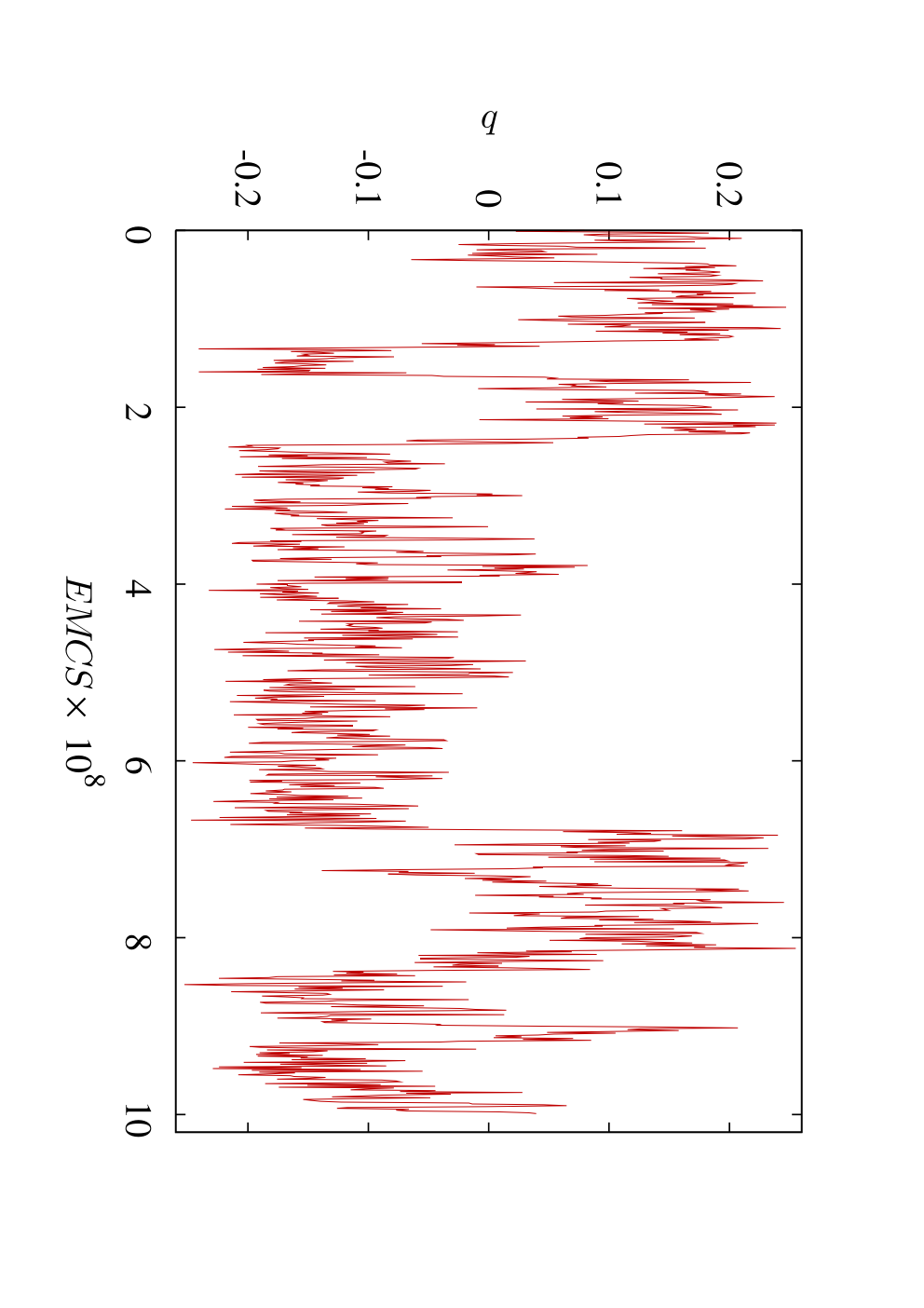
We believe that this discussion clearly shows that it is safe to use for an equilibrium analysis the data from the bin (i.e. the last half of the simulation), since it is fully thermalized.
IV Results for model
We show in Fig. 2 the correlation length in units of as a function of for the three-dimensional model. In the high-temperature regime the curves for different lattice sizes are well separated: for increasing the different curves approach, and for values of close to they seem to have merged in a single curve. In the limits of our statistical accuracy, we do not see any sign of a splitting of the curves in the high- phase (a crossing point at and a splitting in both the low and in the high- phase is the usual signature of a usual phase transition): such a merging (without an eventual splitting) for increasing is what would happen in a Kosterlitz-Thouless transition (KT, see for example Ref. KOSTERLITZ-THOULESS).
The first (of the many) delicate issue about this potential behavior concerns thermalization of the system: we have to be sure that we are not being mislead by the fact that we have not thermalized the larger lattice sizes (this could produce an effect hiding a crossing in the high- region). This is why we have studied, and discussed before, thermalization in detail: the thermalization checks described in Section III make us confident that we have reached equilibrium for all the lattice sizes that we have considered. We should not forget that there are other possible issues that could hide from us, even in a very large scale simulation like the one discussed here, the asymptotic result: we could need for example a better statistical accuracy to discriminate a weak crossing, or we could need large lattices to see the crossing appearing, or we could need to go to higher values. The issue of a very weak transition is a very delicate one, and reliable statements must be phrased with great care. Here we claim that a KT scenario is a possible choice given the data that we have been able to measure in ,
In a KT scenario the quantity is expected to remain invariant in a finite low-temperature region adjacent to the critical point. One way to be quantitative about that is to compute the crossing points for the dimensionless quantity , see Eq. 11. In Fig. 3, we plot the cumulant for several lattice sizes. The curves for different lattice sizes cross close to (look for example at the and the lattices), at a temperature where the curves for on different lattice sizes did not yet merge (i.e. where the correlation length has the high- behavior). The region of the crossing is quite narrow, so that is very implausible that the scaling corrections to (usually larger than that of ) will shift the crossings as much as to get them close to . Therefore, under our numerical accuracy, we do observe that remains invariant in an interval of temperatures lower than that of the crossings of the cumulant.
The features we have described are consistent with a transition of the KT type.KOSTERLITZ-THOULESS Nevertheless, as we have discussed before, many possible effects could lead to difficult conclusions (for example the value of the lower critical dimension to be slightly smaller than three). It is clear, in any case, that in we are indeed sitting very close to the lower critical dimension.
V Results for the model
The authors of Ref. GLASSY-POTTS, where the CRPPG model that we investigate here was proposed, found that the four-dimensional CRPPG undergoes a transition to a spin-glass phase at (by analyzing lattices of size and ).
In order to analyze the transition, we study here the scaling behavior of quantities as and , that are expected to be -independent at the critical point. In Fig. 7 we plot the correlation length in units of the lattice size as a function of . The reweighting extrapolations of these quantities for pairs of lattices and do intersect in the region around . In order to be sure of the existence of the crossing we have thermalized lattices of linear size and deep in the low-temperature region: the normalized correlation length of the larger lattice is well above the one of the smaller lattice for values ranging from to .

In Fig. 8 we zoom the region closer to our putative crossing. In this region we have also thermalized lattice of linear size , and we include the data in the figure and in our analysis.

In Table 3 we give the values of the crossing points obtained by the crossing of the curves. Already from Fig. 8 it is clear that the accuracy of the size-dependent estimates is not high enough to allow to estimate scaling corrections. This is since reaching thermal equilibrium for was not in the scope of our numerical simulation (bound to run on a single FPGA chip), while lattices with linear size would have probably been too small to show true asymptotic scaling corrections.
| 8 | 12 | 1.41(1) | 0.47(2) | 1.1(1) | -0.35(3) | 2.6(2) |
|---|---|---|---|---|---|---|
| 8 | 16 | 1.41(1) | 0.47(1) | 1.1(2) | -0.33(2) | 2.5(4) |
| 12 | 16 | 1.41(1) | 0.46(2) | 1.0(4) | -0.29(5) | 2.4(9) |
Since the cumulant scales like at the critical point, it might have played the same role than (by using Eq. 11). However, we find that it has much larger scaling corrections than , and that these corrections shift the crossing points to higher temperatures, out of the range that we have analyzed (and where we believe the real asymptotic critical behavior can be observed). We have therefore not used in our study of the critical point. Our results compare fairly with the ones obtained in Ref. GLASSY-POTTS by analyzing systems of linear sizes and ( must be renormalized since our Hamiltonian differs by a factor from the one of Ref. GLASSY-POTTS).
To obtain the critical exponents we consider the operators and , whose associated exponents, see Eq. 10, are and . Taking the logarithm of the quotients of these expectation values at the crossing points of , we obtain the effective size-dependent exponents that we show in Table 3. We can summarize our best estimate for the exponents as , , , and : these error are statistical in nature and cannot, obviously, fully take care of the systematic effects.
As was happening in the determination of the value of the critical coupling, the estimated exponents lack the precision necessary for obtaining a reliable infinite volume extrapolation. Ref. GLASSY-POTTS was quoting a value of in the range between and , obtained from the study of the overlap susceptibility in the warm phase of a lattice . Although our estimate is not very close to this value, it is clear that we are still dealing with lattice of intermediate size, and that a careful analysis of scaling corrections, that we hope will soon be possible, will probably lead to reconcile these results. Our results should characterizes, if universality holds, the spin glass transition to a Potts Glass, independently from the detailed model one selects.
Finally, we also show in table 3 the finite-size estimates of the universal quantity , i.e. evaluated at the critical coupling.
VI Conclusions
We have presented a numerical study of the -state CRPPG in , and, for the first time, in : we have used Monte Carlo simulations, reweighting techniques and a finite size scaling analysis. In our evidence clearly shows that we are very close to the lower critical dimension, and suggests that a Kosterlitz-Thouless like behavior is possible, even if we could be dealing with a transient effect. In we are able to collect a large number of thermalized samples for systems defined on large lattices, of linear size . Thanks to such a large scale numerical simulation we are able to qualify the spin-glass transition first found in Ref. GLASSY-POTTS, and we obtain size-dependent estimates of the critical coupling, of the critical exponents and and of the scale-invariant quantity
In both cases, the use of a FPGA gives us the power needed to achieve thermalization, a target very ambitious for standard computers. We have been very careful in checking thermalization, and also thanks to the built-in symmetry of the CRPPG we have succeeded in this task.
Acknowledgments
Numerical computations have been performed at BIFI. We acknowledge partial financial support from CAM-UCM and UCM-BSCH, and from MEC through research contracts FIS2006-08533-C03 and TEC2007-64188. J. L. Velasco is a DGA fellow. We thank Stefano Mossa, Giorgio Parisi and Cristina Picus for a number of conversations about the Glassy Potts models and more. We thank Raffaele Tripiccione and all the JANUS Collaboration for a continuous help that could not have been more important for us.
The FPGA device
The problem of the glassy state, for example, is a typical problem of very high complexity. A large (maybe infinite) number of time scales is involved, and numerical simulations have to try to give hints about dynamics at very long times: very large correlation and thermalization times imply that, already on lattices of medium size, a huge computational effort is required. This is a typical situation where conventional computers could be not enough to do the job.
The use of FPGA programmable chips for the simulation of spin systems has been proposed several years agoSUE: conventional computers are not optimized towards the computational tasks relevant for our typical calculation, and a FPGA can be programmed (at run time) in order to optimize the execution of the specific problem that one wants to solve.
FPGA devices comes with numerous embedded and sizable memory blocks (RAM blocks), and thousands of configurable logic blocks with programmable interconnections. A configurable logic blocks can be programmed to perform complex logic operations and provide storage (flip-flop registers) at the same time.
A number of features that characterize our model are indeed optimal for being dealt with by a FPGA: we have discrete variables that can take a small number of values (four for our system), and the interaction is local in physical space. The Metropolis algorithm and the random number generators discussed in Section III.3 have been implemented in the FPGA in a very effective way.
RAM blocks have a natural (width depth) grid structure. A cubic matrix of bits can be obtained by stacking many of them, and access to all of them with the same memory address corresponds to addressing an entire plane in a grid. We consider one such structure per each bit needed to represent fields (and interactions) defined on the sites of a simple cubic lattice.
Locality of interactions (nearest neighbors) allows for a high grade of internal parallelism: in a checkerboard scheme, all black or all white sites of a lattice plane can be updated simultaneously (i. e. at the same clock cycle). Moreover, when simulating two real replicas and mixing black (white) sites of a system with white (black) ones of its replica, all sites in a plane can be processed in parallel. Simultaneous local updates can then be performed by replicating small computation cells, each executing the few simple logical operations to compute local energies, and including a 32 bit comparator for the Metropolis test. Precomputed transition probabilities (that allows to avoid lengthy computations of transcendental functions) are stored as several small look-up tables in configurable logic (distributed RAM), and addressed by the computed energy variations values (each look-up tables serves two distinct computation cells). The iterative processes involving 32 bit integer arithmetics for random number generators have also been parallelized, by cascading many 32 bit integer adders and xors, and allowing for the generation of hundreds of 32 bit random numbers per clock cycle. For further details, see Ref. IANUS2.
We use the FPGA device Virtex 4/LX200, manufactured by Xilinx. Depending on lattice size and number of parallel updates (between and ) our designs run at clock speeds between and MHz.
In Ref. IANUS2 its performances have been compared with the ones of a GHz Pentium IV device: for the model the FPGA performs 1800 times faster than a Pentium, while this factor is in .
References
- (1) E. Gardner, Nucl. Phys. B 257, 747 (1985)
- (2) D. Elderfield and D. Sherrington, J. Phys. C 16, L497 (1983).
- (3) D. Elderfield and D. Sherrington, J. Phys. C 16, L971 (1983).
- (4) D. J. Gross, I. Kanter and H. Sompolinsky, Phys. Rev. Lett. 55, 304 (1985).
- (5) H. Nishimori and M. J. Stephen, Phys. Rev. B 27, 5644 (1983).
- (6) E. Marinari, S Mossa and G. Parisi, Phys. Rev. B 59 8401 (1999).
- (7) S. Franz, M. Mézard, F. Ricci-Tersenghi, M. Weigt and R. Zecchina, Europhys. Lett. 55, 465 (2001).
- (8) A. Cavagna, I. Giardina and T. S. Grigera, Europhys. Lett. 61, 74 (2003); J. Chem. Phys. 118, 6974 (2003).
- (9) F. Krzakala and L. Zdeborová, Potts Glass on Random Graphs, preprint arXiv:0710.3336.
- (10) K. Binder and J. D. Reger, Adv. Phys. 41, 547 (1992).
- (11) See e.g. M. Mézard, G. Parisi, and M. A. Virasoro, Spin Glass Theory and Beyond (World Scientific, Singapore, 1987).
- (12) D. J. Gross and M. Mézard, Nucl. Phys B 240, 431 (1984).
- (13) T. R. Kirkpatrick and P. G. Wolynes, Phys. Rev. B 36, 8552 (1987).
- (14) T. R. Kirkpatrick and D. Thirumalai, Phys. Rev. B 37, 5342 (1988).
- (15) W. Götze and L. Sjögren, Rep. Prog. Phys. 55, 241 (1992).
- (16) J. P. Bouchaud, L. F. Cugliandolo, J. Kurchan and M. Mézard, in Spin Glasses and Random Fields, edited by A.P. Young (World Scientific, Singapore, 1997).
- (17) K. Binder, in Spin Glasses and Random Fields, edited by A.P. Young (World Scientific, Singapore, 1997).
- (18) J. R. Banavar and M. Cieplak, Phys. Rev. B 39, 9633 (1989).
- (19) J. R. Banavar and M. Cieplak, Phys. Rev. B 40, 4613 (1989).
- (20) M. Scheucher, J. D. Reger, K. Binder, and A. P. Young, Phys. Rev. B 42, 6881 (1990).
- (21) M. Scheucher and J. D. Reger, Phys. Rev. B 45, 2499 (1992).
- (22) M. Reuhl, P. Nielaba, and K. Binder, Eur. Phys. J. B 2, 225 (1998).
- (23) O. Carmesin and K. Binder, J. Phys. A 21, 4053 (1988).
- (24) R. R. P. Singh, Phys. Rev. B 43, 6299 (1991).
- (25) B. Lobe, W. Janke, and K. Binder, Eur. Phys. J. B 7, 283 (1999).
- (26) L. W. Lee, H. G. Katzgraber and A. P. Young, Phys. Rev. B 74, 104416 (2006)
- (27) C. Brangian, W. Kob, and K. Binder, Europhys. Lett. 59, 546 (2002).
- (28) C. Brangian, W. Kob, and K. Binder, J. Phys. A 36, 10847 (2003).
- (29) M. P. Eastwood and P. G. Wolynes, Europhys. Lett. 60, 587 (2002).
- (30) G. Toulouse, Communications on Physics 2, 115 (1977).
- (31) D.M. Carlucci, Phys. Rev. B 60 9862 (1999).
- (32) F. Belletti, M. Cotallo, A. Cruz, L. A. Fernández, A. Gordillo, A. Maiorano, F. Mantovani, E. Marinari, V. Martin-Mayor, A. Muñoz-Sudupe, D. Navarro, S. Perez-Gaviro, J. J. Ruiz-Lorenzo, S. F. Schifano, D. Sciretti, A. Tarancón, R. Tripiccione, J. L. Velasco, Computer Physics Communications 178 (3), 208 (2008).
- (33) E. Marinari, G. Parisi and J. J. Ruiz-Lorenzo, in Spin Glasses and Random Fields, edited by A.P. Young (World Scientific, Singapore, 1997).
- (34) B. Cooper, B. Freedman and D. Preston, Nucl. Phys. B 210, 210 (1982).
- (35) D. Amit and V. Martin-Mayor, Field Theory, the Renormalization Group and Critical Phenomena, (World-Scientific Singapore, third edition, 2005).
- (36) M. Falcioni, E. Marinari, M. L. Paciello, G. Parisi and B. Taglienti, Phys. Lett. B 108, 331 (1982).
- (37) A. M. Ferrenberg and R.H. Swendsen, Phys. Rev. Lett. 61, 2635 (1988).
- (38) H. G. Ballesteros, L. A. Fernández, V. Martin-Mayor, A. Muñoz-Sudupe, G. Parisi and J. J. Ruiz-Lorenzo, Nucl. Phys. B 512, 681 (1998).
- (39) H. G. Ballesteros, L. A. Fernández, V. Martin-Mayor and A. Muñoz Sudupe, Phys. Lett. B 378, 207 (1996).
- (40) H. G. Ballesteros, L. A. Fernández, V. Martin-Mayor and A. Muñoz Sudupe, Nucl. Phys. B 483, 707 (1997).
- (41) G. Parisi and F. Rapuano, Phys. Lett. B 157, 301 (1985).
- (42) J. M. Kosterlitz and D.J. Thouless, J. Phys. C 6, 1181 (1973).
- (43) A. Cruz, J. Pech, A. Tarancón, P. Tellez, C. L. Ullod, C. Ungil, Comput. Phys. Commun. 133, 165 (2001).