Breathers in inhomogeneous nonlinear lattices : an analysis via centre manifold reduction.
Abstract
We consider an infinite chain of particles linearly coupled to their nearest neighbours and subject to an anharmonic local potential. The chain is assumed weakly inhomogeneous, i.e. coupling constants, particle masses and on-site potentials can have small variations along the chain. We look for small amplitude and time-periodic solutions, and in particular spatially localized ones (discrete breathers). The problem is reformulated as a nonautonomous recurrence in a space of time-periodic functions, where the dynamics is considered along the discrete spatial coordinate. Generalizing to nonautonomous maps a centre manifold theorem previously obtained for infinite-dimensional autonomous maps [Jam03], we show that small amplitude oscillations are determined by finite-dimensional nonautonomous mappings, whose dimension depends on the solutions frequency. We consider the case of two-dimensional reduced mappings, which occurs for frequencies close to the edges of the phonon band (computed for the unperturbed homogeneous chain). For an homogeneous chain, the reduced map is autonomous and reversible, and bifurcations of reversible homoclinics or heteroclinic solutions are found for appropriate parameter values. These orbits correspond respectively to discrete breathers for the infinite chain, or “dark” breathers superposed on a spatially extended standing wave. Breather existence is shown in some cases for any value of the coupling constant, which generalizes (for small amplitude solutions) an existence result obtained by MacKay and Aubry at small coupling [MA94]. For an inhomogeneous chain the study of the nonautonomous reduced map is in general far more involved. Here this problem is considered when the chain presents a finite number of defects. For the principal part of the reduced recurrence, using the assumption of weak inhomogeneity, we show that homoclinics to exist when the image of the unstable manifold under a linear transformation (depending on the sequence) intersects the stable manifold. This provides a geometrical understanding of tangent bifurcations of discrete breathers commonly observed in classes of systems with impurities as defect strengths are varied. The case of a mass impurity is studied in detail, and our geometrical analysis is successfully compared with direct numerical simulations.
1 Introduction
It is now well established that many nonlinear networks of interacting particles sustain time-periodic and spatially localized oscillations commonly denoted as discrete breathers. In spatially periodic systems, breathers are also called intrinsically localized modes [ST88] in distinction to Anderson modes of disordered linear systems [And58]. The properties of discrete breathers have been analyzed in an important number of numerical works (see the reviews [FW98, VMZ03, DLHMS04]) and their existence in periodic systems has been proved analytically in different contexts, see [MA94, Aub98, SM97, AS98, AKK01, Pan05, Fla95, Jam03] and their references. In the context of numerical simulations or experiments discrete breathers often denote a larger class of spatially localized oscillations, such as metastable states, oscillations with a certain degree of periodicity, or even chaotic oscillations interacting with a noisy extended background [IKSF04, GLC05]. Nonlinear waves of this type are now actually detected in real materials [SS04, Swa99, SES99, EH02, Man06] and also generated in artificial systems such as Josephson junction arrays, micromechanical cantilever arrays and coupled optical waveguides (see references in [CFK04]). They are thought to play a role in various physical processes such as the formation of local fluctuational openings in the DNA molecule [PB89, Pey04], which occurs in particular during thermal denaturation experiments.
Beyond spatially periodic systems, it is a fundamental and challenging problem to understand breather properties in nonlinear and inhomogeneous media, such as non-periodic or disordered crystals, amorphous solids and biological macromolecules. For example the interplay between nonlinearity and disorder can provide an alternative interpretation for slow relaxation processes in glasses [KA99-00]. In quasi-one-dimensional media, moving localized waves interacting with impurities [KBS94, CPAR02, FPM94], extended defects [TP96] or local bends of the lattice (see [CK04] and its references) can remain trapped and release vibrational energy at specific sites.
The modelling of thermal denaturation of DNA and the analysis of its local fluctuational openings, also known as denaturation bubbles, represents another problem where heterogeneity is important. In order to describe these phenomena, a nonlinear model at the scale of the DNA base pair has been introduced by Peyrard and Bishop [PB89] and further improved by Dauxois et al [DPB93]. The model describes the stretching of the H-bonds between two bases, in the th base pair along a DNA molecule (a large value of corresponding to a local opening). Each bond fluctuates in an effective anharmonic potential and interacts with its nearest-neighbours. The model is described by an Hamiltonian system, and can be coupled with a thermostat to study the effect of thermal noise in denaturation experiments. This model accurately describes the thermal denaturation of real DNA segments provided their heterogeneity is taken into account [CG98] (for example, the dissociation energy of AT and GC base pairs are different). The Hamiltonian of the system reads
| (1) |
where is a Morse potential depending on the base pairs sequence . The case yields a particular case of Klein-Gordon lattice, i.e. the model consists in a chain of anharmonic oscillators with harmonic nearest-neighbours coupling. For parameters corresponding to real DNA sequences, Langevin molecular dynamics of (1) have shown that some locations of discrete breathers heavily depend on the sequence and seem to coincide with functional sites in DNA [KRBCU04], but at the present time this conclusion remains controversial [vECLP06].
From a mathematical point of view, Albanese and Fröhlich have proved the existence of breathers for a class of random Hamiltonian systems describing an infinite array of coupled anharmonic oscillators [AF91] (see also the earlier work [FSW86] of Fröhlich et al concerning quasiperiodic localized oscillations). These breather families can be parametrized by the solutions frequencies, which belong to fat Cantor sets (i.e. with nonzero Lebesgue measure) of asymptotically full relative measure in the limit of zero amplitude. These solutions are nonlinear “continuations” of a given Anderson mode from the limit of zero amplitude, and the gaps in their frequency values originate from a dense set of resonances present in the system. For disordered Klein-Gordon lattices, complementary numerical results on the continuation of breathers with respect to frequency or the transition between breathers to Anderson modes are available in [KA99-00, AMM99].
In addition, the existence of breathers in inhomogeneous Klein-Gordon lattices (with disordered on-site potentials) has been proved by Sepulchre and MacKay [SM98, SM97] for small coupling . The proof is based on the continuation method previously introduced by MacKay and Aubry [MA94] for an homogeneous chain (method considerably generalized in [SM97]). For the system reduces to an array of uncoupled non-identical anharmonic oscillators, and the simplest type of discrete breather consists of a single particle oscillating while the others are at rest. Under a nonresonance condition [SM98, SM97], this solution can be continued to small values of (in most cases at fixed frequency) using the implicit function theorem, yielding a spatially localized solution.
In this paper we provide complementary mathematical tools for studying time-periodic oscillations (not necessarily spatially localized) in inhomogeneous infinite lattices. The theory is developed in a very general framework, and applied to breather bifurcations in inhomogeneous Klein-Gordon lattices as lattice parameters and breather frequencies are varied. We start from a general Klein-Gordon lattice with Hamiltonian
| (2) |
(case of (1) with more general inhomogeneities). The potential is assumed sufficiently smooth in a neighbourhood of with , . The general theory is a priori valid for small inhomogeneities and small amplitude oscillations. In particular, in our application to system (2) we assume , , , to be close (uniformly in ) to positive constants. However, considering an example of Klein-Gordon lattice with a mass defect, we check using numerical computations that our tools remain applicable up to strongly nonlinear regimes, and sometimes for a large inhomogeneity.
Our analysis is based on a centre manifold reduction and the concept of spatial dynamics. This concept was introduced by K. Kirchgässner [Kir82] for nonlinear elliptic PDE in infinite strips, considered as an (ill-posed) evolution problem in the unbounded space coordinate, and locally reduced to a finite-dimensional ODE on an invariant centre manifold. This idea was transposed to the context of travelling waves in homogeneous infinite oscillator chains by Iooss and Kirchgässner [IK00], and centre manifold reduction has been subsequently applied to the analysis of travelling waves and pulsating travelling waves in different one-dimensional homogeneous lattices [Ioo00, JS05, IJ05, Sir05, PR05, IP06]. Indeed, looking for travelling waves in an oscillator chain yields an advance-delay differential equation (a system of such equations in the case of pulsating travelling waves), which can be reformulated as an infinite-dimensional evolution problem in the moving frame coordinate, and locally reduced to a finite-dimensional ODE under appropriate spectral conditions.
In reference [Jam01], one of us has proved the existence of breathers in Fermi-Pasta-Ulam (FPU) lattices using a similar technique in a discrete context. The dynamical equations for time-periodic solutions were reformulated as an infinite-dimensional recurrence relation in a space of time-periodic functions, and then locally reduced to a finite-dimensional mapping on a centre manifold, where breathers corresponded to homoclinic orbits to . A general centre manifold theorem for infinite-dimensional maps with unbounded linearized operator has been proved subsequently [Jam03] and has been used to analyze breather bifurcations in diatomic FPU lattices [JN04, JK07] and spin lattices [Nob04]. More generally, the dynamical equations of many one-dimensional lattices can be reformulated as infinite-dimensional maps in loop spaces as one looks for small amplitude time-periodic oscillations ([Jam03], section 6.1).
As shown in the present paper, the centre manifold reduction theorem readily applies to homogeneous Klein-Gordon lattices, where , , , in (2) and . This reduction result rigorously justifies (in the weakly nonlinear regime) a formal one-Fourier mode approximation previously introduced in reference [BCKRBW00]. The equations of motion read
| (3) |
Looking for time-periodic solutions (with frequency ) and setting , (3) can be formulated as an (ill-posed) recurrence relation in a space of -periodic functions. Using the theorem of reference [Jam03], one can locally reduce the problem to a finite-dimensional mapping on a centre manifold whose dimension depends on the frequency . More precisely, equation (3) linearized at admits solutions in the form of linear waves (phonons) with , whose frequency satisfies the dispersion relation
| (4) |
The frequencies lie in a band with . In the nonlinear case, the dimension of the centre manifold depends on how many multiples of belong to (or are close to) the phonon band. When or (with no additional resonance), the centre manifold is two-dimensional if solutions are searched even in time, which reduces (3) locally to a two-dimensional reversible mapping on the centre manifold. For appropriate parameter values, this map admits small amplitude homoclinic solutions to corresponding to breather solutions of (3). Breather solutions in this system have been proved to exist by MacKay and Aubry [MA94] for small values of the coupling parameter . Known regions of breather existence are considerably extended here, since we prove the existence of small amplitude breathers for arbitrary values of in some cases and for frequencies close to the phonon band edges (see theorem 7 p.7). In addition we prove the existence of “dark breather” solutions, which converge towards a nonlinear standing wave as and have a much smaller amplitude at the centre of the chain. These solutions correspond to heteroclinic orbits of the reduced two-dimensional map.
Furthermore, we extend this analysis to the case when small lattice inhomogeneities are present. The dynamical equations of the inhomogeneous system (2) take the form
| (5) |
and time-periodic solutions can be obtained as orbits of a nonautonomous map , where the nonconstant lattice parameters are embedded in a multicomponent parameter . Fixing , , , , we consider the case when constant lattice parameters are perturbed by uniformly small sequences , , , . We prove (see theorem 3 p.3) that small amplitude time-periodic solutions with frequencies close to or are determined by a two-dimensional nonautonomous map. Moreover, we generalize this reduction result in the case when several multiples of are close to the band , which yields a higher-dimensional reduced problem (see theorem 4 p.4).
In fact we prove this type of reduction result in a very general framework, for infinite-dimensional mappings with small nonautonomous perturbations, considered in a neighbourhood of a non-hyperbolic fixed point, or close to a bifurcation. The linear autonomous part of the map must satisfy a property of spectral separation (see theorem 1 p.1), but a large number of one-dimensional lattices with finite-range coupling fall within this category. We obtain a direct proof of the reduction result by observing that any nonautonomous mapping can be seen as a projection of an extended autonomous mapping, to which the centre manifold theorem of reference [Jam03] can be applied under appropriate assumptions. The centre manifold of the extended map is infinite-dimensional, but this case is also covered in [Jam03]. The reduced nonautonomous mapping for the original system can be interpreted as a projection on a finite-dimensional subspace of the extended autonomous mapping restricted to the invariant centre manifold.
We use this reduction result to analyse the case when equation (5) presents a mass defect at a single site, all other lattice parameters being independent of . In that case, the linearized problem admits a spatially localized mode (usually denoted as an impurity mode), and a nonlinear continuation of this mode can be computed [FPM94], corresponding to a Lyapunov family of periodic orbits. Klein-Gordon systems with a coupling defect or a harmonic impurity in the on-site potential share similar characteristics [CPAR02], as well as nonlinear lattices with a different type of nonlinearity [KZK97]. In addition to this simple localization phenomenon, single impurities can have more complex effects in a nonlinear system. Indeed it is a common feature to observe a complex sequence of tangent bifurcations between (deformations of) site-centered and bond-centered breathers in some neighbourhood of the defect as the strength of an impurity is varied [CK04, KZK97]. Using numerical computations we show some examples of such bifurcations in the present paper, as one varies the strength of a mass defect in system (5). From a physical point of view it is quite important to understand how a local change in the lattice parameters modifies the set of spatially localized solutions. For example, this could contribute to explain how a mutation at a specific location of an homogeneous sequence of (artificial) DNA would modify the structure of fluctuational openings [KRBCU04].
This paper provides a qualitative explanation of such tangent bifurcations, which reveals also very precise quantitatively when compared with numerical simulations of the Klein-Gordon model. According to the previously described reduction theorem, for a small mass defect of size , small amplitude breather solutions of (5) with frequencies below (and close to) are described by a two-dimensional nonautonomous mapping . Here we only study the principal part of the reduced mapping as . We show that this truncated reduced map admits an homoclinic orbit to (corresponding to an approximate breather solution for the oscillator chain) if, for , the image of the unstable manifold of under a certain linear shear intersects its stable manifold. The linear shear is -close to the identity. When the on-site potential is soft, these manifolds have very complicated windings characteristic of homoclinic chaos, hence the set of their intersections changes in a complex way as the linear shear varies, or equivalently as one varies the mass defect. This phenomenon explains the existence of the above mentioned tangent bifurcations, at least for small defect sizes, and for small amplitude breathers with frequencies close to the phonon band. In addition, we show (by comparison with direct numerical simulations of the Klein-Gordon model) that this picture remains valid quite far from the weakly nonlinear regime. Let us note that, to obtain an exact solution of (5) from an orbit of the truncated map, it would be necessary to control the effect of higher order terms (with respect to , , ) present in the full reduced mapping and prove the persistence of this solution. This problem is not examined here from the analytical side, but we compare instead numerically computed solutions of (5) with approximate solutions deduced from the truncated map. The very good agreement leads us to conjecture that most of the homoclinic bifurcations existing for the truncated problem persist for the full reduced system.
Lastly we consider the more general case when system (5) admits a finite number of defects, i.e. perturbations , , , have a compact support (as above these perturbations are assumed to be small, of order ). We show that the approach developped for a single impurity can be extended to this case (see lemma 7 p.7), where the linear shear is replaced by a more general linear near-identity transformation . The linear transformation provides a useful tool for studying breather bifurcations in Klein-Gordon lattices with a finite number of impurities, as for the single impurity case that we have analyzed in detail. By computing the principal part of as is small and frequencies are close to , we show that the effect of the parameter sequence on the set of small amplitude breather solutions should mainly depend on weighted averages of the defects values.
The outline of the paper is as follows. Section 2 presents the centre manifold reduction theory for time-periodic oscillations in weakly inhomogeneous nonlinear lattices. We treat the case of Klein-Gordon lattices in detail in sections 2.1 and 2.3, and formulate the reduction theory in a much more general setting in section 2.2. Section 3 concerns spatially homogeneous Klein-Gordon lattices. Existence theorems for small amplitude breather and dark breather solutions are deduced from the dynamics of two-dimensional reversible maps on invariant centre manifolds. The case of weakly inhomogeneous Klein-Gordon chains is considered in section 4, where the truncated reduced map is analyzed for a finite number of defects. A geometrical condition for the existence of homoclinic orbits to is derived in section 4.2, and some homoclinic bifurcations are studied in detail in section 4.1 for a single mass defect. In the latter case, breather solutions are numerically computed in section 5 and the results are successfully compared with our analytical findings.
2 Reduction result for small inhomogeneities
In this section we consider system (5) in the limit of small inhomogeneities. We show that all small amplitude time-periodic solutions are determined by a finite-dimensional nonautonomous map, whose dimension depends on the frequency domain under consideration. For this purpose we reformulate (5) as a map in a loop space, perturbed by a small nonautonomous term (section 2.1). Then we prove in section 2.2 a general centre manifold reduction theorem for infinite-dimensional maps with small nonautonomous perturbations. This result is based on the centre manifold theorem proved in reference [Jam03] for autonomous systems. Our general result is applied to the inhomogeneous Klein-Gordon lattice, which yields the above mentioned reduction result (section 2.3).
2.1 The Klein-Gordon system as a map in a loop space
We set in equation (5), where is -periodic in (hence is time-periodic with frequency ). The constant being fixed, we also define . Equation (5) becomes
| (6) |
where and , , , . The sequences , , will be assumed sufficiently small in , where is the classical Banach space of bounded sequences on , equiped with the supremum norm. To simplify the notations, we shall drop the tilde in the sequel when referring to the renormalized potential . Moreover we shall use the shorter notations when referring to sequences .
To analyze system (6) we use the same approach as in reference [Jam03] for spatially homogeneous systems. We reformulate (6) as a (nonautonomous) recurrence relation in a space of -periodic functions of , and locally reduce the (spatial) dynamics to one on a finite-dimensional centre manifold. We restrict our attention to the case when is even in in order to deal with lower-dimensional problems. More precisely, we assume for all , where and denotes the classical Sobolev space of -periodic functions ().
Since our analysis concerns small amplitude solutions and small inhomogeneities, the first step consists in studying the linearized system at when are fixed equal to . In that case equation (6) yields
| (7) |
Now we rewrite the problem as an infinite-dimensional linear mapping. For this purpose we introduce , where . Equation (7) can be written
| (8) |
where
| (9) |
and equation (8) holds in . The operator is unbounded in (of domain ) and closed (we omit the additional parameter in the notation ).
The spectrum of consists in essential spectrum at the origin and an infinite number of eigenvalues () depending on , , and satisfying the dispersion relation
| (10) |
(it follows that is either real or has modulus one). Equation (10) is directly obtained by setting in equation (7). The invariance in (10) originates from the invariance in (7). In the sequel we shall note the solution of (10) satisfying and . Clearly is real negative for large enough and . Moreover accumulates at as . It follows that the number of eigenvalues of on the unit circle is finite for any value of the parameters .
In addition, the eigenvalues defined by (10) lie on the unit circle when . This property as a simple interpretation. Multiplying (10) by , setting and , one finds the usual dispersion relation (4). Consequently, if lies inside the phonon band for some , then admits a pair of eigenvalues on the unit circle determined by the dispersion relation (4). This condition on is equivalent to prescribing .
Now let us describe the spectrum of near the unit circle when is fixed and is varied. As we shall see, the number of eigenvalues of on the unit circle changes as crosses an infinite sequence of decreasing critical values . Small amplitude solutions of the nonlinear system bifurcating from will be found near these critical frequencies.
We begin by studying the evolution of each pair of eigenvalues , as varies. Firstly, one can easily check that are independent of , real positive and lie strictly off the unit circle.
Secondly we consider the case . For , are real negative and lie strictly off the unit circle. When decreases, they approach the unit circle and one has for (this corresponds to a frequency at the top of the phonon band, for a wavenumber ). At this critical parameter value, is a double non semi-simple eigenvalue of . For , lie on the unit circle, and approach as decreases. One has for , and then is a double non semi-simple eigenvalue of (this corresponds to a frequency at the bottom of the phonon band, for a wavenumber ). For , are real positive and lie strictly off the unit circle.
Now let us qualitatively describe the evolution of the whole spectrum of . When the spectrum of lies strictly off the unit circle (both inside and outside). When decreases, the eigenvalues approach the unit circle for all . As the first critical value is reached, the eigenvalues collide and yield a double (non semi-simple) eigenvalue , while the remaining part of the spectrum is hyperbolic. When is further decreased, two different situations occur depending on the value of .
For , are the only eigenvalues on the unit circle for . One has at the second critical value . When is further decreased, are real positive and lie strictly off the unit circle. One has at the third critical value . The situation is sketched in figure 1.

The case is different, since are the only eigenvalues on the unit circle in the smaller frequency range . Indeed one has at second critical value . For and the spectrum of on the unit circle consists in two pairs of simple eigenvalues . In the interval other eigenvalues may collide at depending on the value of . The situation is sketched in figure 2.

In what follows we restrict our attention to the neighbourhood of critical frequencies with , and . This leads us to consider the small parameter defined by . As equals one of the critical frequencies , the spectrum of on the unit circle only consists in a double eigenvalue or . For or , the above spectral analysis shows that the fixed point of (8) is hyperbolic when or . In this case, when nonlinear effects will be taken into account, we shall see that the stable and unstable manifolds , may intersect depending on the local properties of the anharmonic potential , leading to the existence of homoclinic orbits to .
System (6) will be analyzed in the limit of small amplitude solutions and for small parameters , . The parameter space will be denoted as . All parameters are embedded in a multicomponent parameter . In addition we denote by the index shift in , i.e. .
Equation (6) can be rewritten in the form of a nonautonomous mapping in a function space. More precisely we have
| (11) |
where , , (for or ) and ,
| (12) |
Equation (11) holds in the Hilbert space . The potential is assumed sufficiently smooth (, with ) in a neighbourhood of . It follows that is () in a neighbourhood of . The operator consists in higher order terms as , i.e. we have , .
We note that (11) is invariant under the symmetry . Moreover the usual invariance under index shifts is broken by the inhomogeneity of the lattice, and replaced by the invariance .
In the next section we prove a general centre manifold reduction theorem for maps having the form (11), under appropriate spectral conditions on and for small nonautonomous perturbations . This analysis relies on the reduction results proved in reference [Jam03] for autonomous maps. To simplify the proof, problem (11) will be considered as a projection of a suitable autonomous mapping to which the centre manifold theorem can be directly applied.
2.2 Centre manifold reduction for nonautonomous perturbations of infinite-dimensional maps
In this section we reformulate the situation of section 2.1 in a general framework, and prove a local centre manifold reduction result for problems of this type. This level of generality is relevant for nonlinear lattices, because the dynamical equations of many one-dimensional lattices can be reformulated as infinite-dimensional maps in loop spaces as one looks for small amplitude time-periodic oscillations. Indeed, if the coupling between sites has finite range (i.e. is coupled to for ), then in general can be obtained locally as a function of using the implicit function theorem (for some examples see e.g. [Jam03], section 6.1, or [JK07]).
To work in a general setting, let us consider a Hilbert space and a closed linear operator of domain , being in general unbounded. We equip with the scalar product , hence is a Hilbert space continuously embedded in .
We denote by a neighbourhood of in and consider a nonlinear map (), where satisfies , . We look for sequences in satisfying
| (13) |
where is a bounded sequence in treated as a parameter. In what follows we shall note the Banach space in which lies. Notice that is a fixed point of (13).
We assume that has the property of spectral separation, i.e. satisfies the assumption (H) described below (in what follows we note the spectrum of a linear operator ).
Assumption (H): The operator has nonempty hyperbolic () and central () spectral parts. Moreover, there exists an annulus () such that the only part of the spectrum of in lies on the unit circle.
The situation corresponding to assumption (H) is sketched in figure 3. Under assumption (H), the hyperbolic part of is isolated from its central part . In particular this allows one to split into two subspaces invariant under , corresponding to respectively. More precisely, and satisfy and .
The invariant subspace is called centre subspace, and is the hyperbolic subspace. The subspace is finite-dimensional when the spectrum of on the unit circle consists in a finite number of eigenvalues with finite multiplicities (we do not need this assumption for the reduction theorem constructed here).
The spectral projection on the centre subspace can be defined in the following way (see e.g. [Kat66])
where denotes the circle of centre and radius (see figure 3). One has , and , where denotes the set of bounded operators from into . In the sequel we note and .

Remark 1
Let us consider the situation of section 2.1 and the linear operator of equation (11). In the case and , the spectrum of on the unit circle consists in a double non semi-simple eigenvalue . Moreover, for the spectrum of on the unit circle consists in a double non semi-simple eigenvalue . In both cases the associated invariant subspace is spanned by , and we have . In addition the unit circle is isolated from the remainder of the spectrum, since the latter is discrete and only accumulates at the origin and at on the real axis. It follows that satisfies assumption (H).
Now we state the centre manifold reduction theorem in the general case. In the sequel we note , .
Theorem 1
Assume that has the property of spectral separation, i.e. satisfies assumption (H). There exists a neighbourhood of in and a map (with , ) such that for all the following holds.
i) If is a solution of (13) such that for all , then for all and satisfies the nonautonomous recurrence relation in
| (14) |
where is defined by
iii) If commutes with a linear isometry then and .
Properties i), ii) reduce the local study of (13) to that of the nonautonomous recurrence relation (14) in the subspace . Note that the dependency of and the reduced map with respect to sequences is nonlocal.
In what follows we give a simple proof of theorem 1 which relies on the fact that the nonautonomous mapping (13) can be seen as a projection of an extended autonomous mapping, to which the centre manifold theorem proved in [Jam03] can be applied. This procedure will explain why the result of theorem 1 can be seen as a centre manifold reduction, since the reduction function will appear as one component of the function having the centre manifold as its graph. The reduced nonautonomous mapping (14) will be interpreted as a projection of the extended autonomous mapping restricted to the invariant centre manifold.
Theorem 1 has been proved in reference [Jam03] in the case of an autonomous mapping, when the sequence is absent or replaced by a simple parameter .
To recover this autonomous case we introduce the additional variable . Note that for any fixed , denotes a bounded sequence in (to simplify the notations we use the symbol instead of ). Given a sequence we also note . Equation (13) can be rewritten
| (15) |
which consists in an autonomous mapping in .
In what follows we apply the theory of reference [Jam03] to system (15). As we shall see the corresponding centre manifold will be infinite-dimensional due to the second component of (15). The case of infinite-dimensional centre manifolds has been treated in reference [Jam03], with the counterpart that theory is restricted to maps in Hilbert spaces. Consequently the first step is to search for in a suitable Hilbert space instead of the Banach space . For this purpose we consider the space of sequences
where . The space defines a Hilbert space equiped with the scalar product , where denotes the usual scalar product on and the associated norm. For all we now search for in the space consisting of real sequences in . Note that , the embedding being continuous.
Since sequences in may be unbounded and is defined on a neighbourhood of in , we replace (15) by a locally equivalent problem
| (16) |
where
is a cut-off function satisfying , for , for , being chosen small enough (with ).
Problem (16) consists in an autonomous mapping in . In order to apply the centre manifold theorem of reference [Jam03] we need to study the spectrum of . One has clearly , where is determined in the following lemma.
Lemma 1
The spectrum of consists of the unit circle.
Proof. Consider the complexification of . Given a sequence and , we look for satisfying
| (17) |
Equation (17) can be solved in a simple manner using Fourier series. Recall that the periodic Sobolev space can be defined as the set of functions in whose Fourier coefficients form a sequence in , where
In the same way its dual space is isomorphic to , where the isomorphism is again given by for all . In addition one has the useful property for all . Now return to equation (17) and consider and . One obtains the equivalent problem in
| (18) |
If then (18) has the unique solution , hence . If is chosen on the unit circle, is a solution for , corresponding to an eigenvector of .
As it follows from lemma 1, consists of the union of with the unit circle. Consequently has the property of spectral separation, i.e. the hyperbolic part of its spectrum is isolated from the unit circle. Moreover the centre subspace of is simply . With these spectral properties at hand, we now apply the centre manifold theorem of reference [Jam03] which states the following.
Theorem 2
There exists a neighbourhood of in and a map (with , ) such that the manifold
has the following properties.
i) is locally invariant under , i.e. if then .
ii) If is a solution of (16) such that for all , then for all (i.e. ) and satisfies the recurrence relation in
| (19) |
where
iii) Conversely, given a solution of (19) such that for all , consider . Then defines a solution of (16) lying on .
iv) If commutes with a linear isometry then and .
The manifold is called a local centre manifold for (16). It is locally invariant under (as stated by property i) ) and the linear isometries of (16). Property iv) expresses the invariance of under the linear isometry of (16).
Now the proof of theorem 1 follows directly from theorem 2. Since is continuously embedded in , defines a map from into . In theorem 1 we choose as a ball of centre in such that and on . Then problems (13) and (16) are equivalent for all , with , and properties i)-ii)-iii) of theorem 1 are directly deduced from properties ii)-iii)-iv) of theorem 2. In addition, since is a solution of (16) for all it follows (by property ii) of theorem 2), and consequently .
2.3 Application to the Klein-Gordon lattice
2.3.1 Reduction result
In this section we apply the reduction theorem 1 to the inhomogeneous Klein-Gordon lattice considered in section 2.1. We recall that the inhomogeneous system (6) has been reformulated as a nonautonomous map in a loop space given by expression (11). All parameters (sequences of heterogeneities and frequency shift ) are embedded in the multicomponent parameter . The problem has exactly the general form (13) (in a particular case when the first component of is constant) and consequently the reduction theorem 1 can be applied to (11). This yields the following result for the original system (6).
Theorem 3
Fix in equation (6), where or (in that case we further assume ). There exist neighbourhoods , and of in , and respectively, and a map (with , ) such that the following holds for all .
i) All solutions of (6) such that for all have the form
where . For , satisfies a recurrence relation
| (20) |
where is . The principal part of reads
| (21) |
| (22) |
For one has
| (23) |
with
| (24) |
| (25) |
In both cases, higher order terms in are and non-local in .
ii) If is a solution of problem (20) or (23) (respectively for or ), such that for all , then satisfies equation (6).
iii) The functions and have the following symmetries
where denotes the half period time shift .
It is straightforward to check that system (6) has the reduction properties i) and ii) described above since the equivalent system (11) satisfies properties i) and ii) of theorem 1 (see remark 1 p.1). However there remains to compute the explicit forms (21) and (24) of the recurrence relations. These expressions do not simply correspond to the two-dimensional mapping (14) rewritten as a second order recurrence relation. In addition we rewrite (14) in normal form, i.e. we perform a polynomial change of variables which simplifies (14) by keeping only its essential terms. These computations will be the object of the next three sections. Property iii) is equivalent to property iii) of theorem 1, where the symmetry is the half period time shift which satisfies .
A possible way of computing the reduced recurrence relation would be to consider the equivalent autonomous mapping (15) and use a classical computation scheme for centre manifolds of autonomous systems (see e.g. [Van89] for a description of the method). The first step consists in computing the Taylor expansion of the reduction function up to a given order. This can be done using a nonlocal equation for (obtained by expressing in (15) as a function of ) and computing the Taylor coefficients of by induction (see [Van89]). The second step is to compute the reduced recurrence relation (19) which is completely determined by .
In the next three sections we shall use a different method yielding simpler computations. Firstly we compute the recurrence relations (21) and (24) in the autonomous case , using the method of reference [Jam03]. Then, using a symmetry argument, we deduce how the leading order part of the reduced equation is modified by the nonautonomous terms of (11).
To end this section we point out a generalization of theorem 3. As it follows from the analysis of section 2.1, the dimension of the centre space of is twice the number of multiples of lying within the band . More precisely, if for , with no additional multiples entering the band, then the centre space is spanned by the corresponding Fourier modes , . As above the following reduction result follows from theorem 1.
Theorem 4
Consider such that for all integers , with no additional multiples in this interval. Fix in equation (6) and note . Consider the subspace of spanned by the Fourier modes and its complementary subspace consisting of orthogonal Fourier modes. There exist neighbourhoods , of in , respectively, and a map (with , ), such that for all , all solutions of (6) such that for all have the form
| (26) |
Moreover, all small amplitude solutions of (6) are determined by a finite-dimensional recurrence relation obtained by projecting (6) on and using the ansatz (26).
2.3.2 Homogeneous case near the lower phonon band edge
In this section we restrict our attention to the case when and . We consider the autonomous case when . Equation (11) now reads
| (27) |
where is given by (9) and
with . System (27) is a reformulation of the equations of motion for the homogenous Klein-Gordon lattice
| (28) |
As in the nonautonomous case (11), system (27) is invariant under the symmetry . Moreover, the invariance of (28) implies that (27) is reversible with respect to the symmetry , i.e. if is a solution then also . In other words, if and are in some neighbourhood of in one has . Lastly, due to the existence of the additional symmetry , it is worthwhile to notice that defines an other reversibility symmetry.
In what follows we use the notations introduced in section 2.2. We recall that the spectrum of on the unit circle consists in a double non semi-simple eigenvalue , and the associated two-dimensional invariant subspace is spanned by the vectors , , with
in the basis . For in some neighbourhood of , (27) admits a two-dimensional local centre manifold (which can be written as a graph over ), locally invariant under (see [Jam03], theorem 1 p. 32). One can write
| (29) |
where and . Moreover, is invariant under and (see [Jam03], theorem 2 p. 34 and section 5.2).
In the sequel we use the notations , and . The spectral projection on reads and we have .
Since is invariant under and , are exchanged by , we have the symmetry property . Consequently, the function has the form
| (30) |
with . Since is invariant under and we have in addition
| (31) |
For , the centre manifold contains all solutions of (27) staying in a sufficiently small neighbourhood of in for all . Their coordinates on are thus given by a two-dimensional mapping which determines all small amplitude solutions when . The reduced mapping is given by
| (32) |
where
| (33) |
| (34) |
One obtains equation (32) using the fact that
for and applying to equation (27) (one has and on ).
Since the reduced mapping inherits the symmetries of (27) [Jam03], commutes with and thus . Moreover, is reversible with respect to the symmetry , i.e. . This yields the identity
This imposes the following structure for the Taylor expansion of at
| (35) |
where coefficients have to be determined. Note that (see [Jam03] p.53 for details).
For determining the unknown coefficients of (35), we first compute the leading order terms in the Taylor expansion of at . This can be done using the fact that is locally invariant under (see [Jam03], theorem 1 p. 32). For , this yields
| (36) |
or equivalently
| (37) |
| (38) |
Thanks to the symmetry property (37), the Taylor expansion of at order takes the form
| (39) |
By an identification procedure we now compute the coefficients in (39), using (38) and the expansion
| (40) |
Identification at order gives
hence since . Identification at order leads to
| (41) |
and identification at order yields
| (42) |
and consequently
As a conclusion, we obtain
| (43) |
2.3.3 Homogeneous case near the upper phonon band edge
In this section we consider the case , in the autonomous case when . Equation (11) takes the form (27), where is given by (9). The spectrum of on the unit circle consists in a double non semi-simple eigenvalue , and the centre space is again spanned by , .
For in some neighbourhood of , there exists a smooth two-dimensional local centre manifold locally invariant under , , and having the form (29). The function having the centre manifold as its graph has the form (30) and shares the property (31). For , the centre manifold contains all solutions of (27) staying in a sufficiently small neighbourhood of in for all . Their coordinates on are then given by a two-dimensional mapping, which determines all small amplitude solutions when .
The operator has the following structure in the basis
and the reduced mapping is given by
| (48) |
where
| (49) |
and is defined by (34). Since the reduced mapping inherits the symmetries of (27), commutes with hence . Moreover, (48) is reversible with respect to the symmetry , which yields the identity
This implies and
| (50) |
where the coefficients have to be determined.
For this purpose, we first compute the leading order terms in the Taylor expansion of at , using the fact that is locally invariant under . Equation (36) yields
| (51) |
| (52) |
The Taylor expansion of at order takes the following form (due to the symmetry property (51))
| (53) |
By an identification procedure we now compute the coefficients in (53), using (52) and the expansion (40). Identification at order gives
hence since . Identification at order leads to
| (54) |
and identification at order yields
| (55) |
and consequently
As a conclusion, we obtain
| (56) |
2.3.4 Inhomogeneous cases
Using the normal form computations performed in the above sections for the autonomous case, one can obtain by perturbation the principal part (20) (or (23)) of the normal form for (or ) in the nonautonomous case. In what follows this computation is described for , the treatment for being completely similar.
Theorem 3 is obtained by applying the reduction theorem 1 to the first order system (11). According to theorem 1-i), small amplitude solutions of (11) have the following form for small
| (61) |
where and denotes the reduction function of theorem 1. In the sequel we shall note .
Let us compute the explicit form of the reduced map (14). For this purpose, one has to use the ansatz (61) in equation (11) and project the latter on the Fourier mode . Setting , the reduced map (14) becomes
| (62) |
| (63) |
where (recall )
| (64) |
and the function is defined by (12).
Since commutes with and , the map commutes with . We have consequently
| (65) |
where the coefficients need to be determined. Now, since in the homogeneous case (see section 2.3.2), we have and , are defined by (45). Consequently we have computed the principal part of the reduced equation (62) in the nonautonomous case.
3 Exact periodic solutions for an homogeneous lattice
Here we consider the case of the homogeneous Klein-Gordon lattice (3), which leads us to system (6) with . Breather solutions have been proved to exist by MacKay and Aubry [MA94] for system (3) with small values of the coupling parameter and nonresonant breather frequencies. Here we prove the existence of small amplitude breathers for arbitrary values of in some cases and frequencies close to the phonon band edges (see theorems 5-i), 6-i) and 7 below). We also prove the existence of dark breather solutions, which converge towards a nonlinear standing wave as and have a much smaller amplitude at the centre of the chain.
Let us start with the case and in (6). By theorem 3, small amplitude solutions of (6) in are determined by the recurrence relation (20). This recurrence becomes autonomous for an homogeneous lattice and takes the form (46). It is important to note that the invariance of (6) in the homogeneous case is inherited by (46) (see [Jam03], section 5.2 and theorem 2). This invariance implies that the two-dimensional map is reversible. Bifurcations of small amplitude homoclinic and heteroclinic solutions have been studied in [Jam03] (section 6.2.3) for this class of maps. This yields the following result for the recurrence relation (46).
Lemma 2
Assume and . For , the recurrence relation (46) has the following solutions.
i) For and , (46) has at least two homoclinic solutions , (and also , ) such that . These solutions have the symmetries , and satisfy , with .
ii) If and have the same sign, (46) has two symmetric fixed points .
iii) For and , (46) has at least two heteroclinic solutions , (and also , ) such that . These solutions have the symmetries and . Moreover, , are as and for bounded values of .
Note that for and (), (46) has no small amplitude homoclinic solution to .
For , typical plots of the stable and unstable manifolds of the fixed point are shown in figure 5 page 5 (nonintersecting case ) and in figures 7 and 12 pages 7 and 12 (intersecting case ).
Theorem 3 ensures that each solution in lemma 2 corresponds to a solution of (6) given by
| (66) |
with in (6). The following result follows (the symmetries of are due to the symmetries of described in lemma 2).
Theorem 5
i) For and , (6) has at least two homoclinic solutions , (and also , ) such that . These solutions satisfy , and have the form
| (67) |
where and . Solutions , correspond to small amplitude breathers with a slow exponential decay as .
ii) If and have the same sign, (6) admits a solution independent of , corresponding to collective in-phase oscillations. It has the form and .
iii) For and , (6) has at least two heteroclinic solutions , (and also , ) such that and . These solutions satisfy and . Moreover, their norms , are as and for bounded values of . Solutions , correspond to small amplitude dark breathers.
In addition, note that for there exists no small amplitude discrete breather with and (since (46) has no small amplitude solution homoclinic to ).
Now we consider the case with . In that case, equation (6) can be locally reduced to the recurrence relation (23), which becomes again autonomous if and has the invariance . This class of recurrence relations has been studied in [Jam03] (section 6.2.3, lemma 7) to which we refer for details. In addition one can note that the recurrence (60) can be recast in the form (46) by setting . The following result for the recurrence relation (60) follows.
Lemma 3
Assume . For , the recurrence relation (60) has the following solutions.
i) For and , (60) has at least two homoclinic solutions , (and also , ) such that . These solutions have the symmetries , and satisfy , with .
ii) If and have the same sign, (60) has a period solution , with .
iii) For and , (60) has at least two heteroclinic solutions , (and also , ) such that . These solutions have the symmetries and . Moreover, , are as and for bounded values of .
In addition, for and () problem (60) has no small amplitude homoclinic solution to . As above, the solutions of the reduced recurrence relation provided by lemma 3 yield the following solutions of (6).
Theorem 6
i) For and , (6) has at least two homoclinic solutions , (and also , ) such that . These solutions satisfy , and have the form
| (68) |
where and . Solutions , correspond to small amplitude breathers with a slow exponential decay as .
ii) If and have the same sign, (6) admits a solution being -periodic in , corresponding to out-of-phase oscillations. It has the form with () and .
iii) For and , (6) has at least two heteroclinic solutions , (and also , ) such that and . These solutions satisfy and . Moreover, their norms , are as and for bounded values of . Solutions , correspond to small amplitude dark breathers.
In addition, for there exists no small amplitude discrete breather with and .
It is worthwhile mentioning that approximate breather solutions of (6) can be obtained in the form of modulated plane waves, using multiscale expansions (see [GM04] and references therein), where the error can be controlled over finite time intervals. The envelope of a modulated wave satisfies the nonlinear Schrödinger (NLS) equation, and does not propagate along the chain when a plane wave with wavenumber or is modulated (its group velocity vanishes). In these two cases the NLS equation is focusing (i.e. time-periodic and spatially localized solutions exist) when and respectively, which coincides (according to theorems 5 and 6) with the parameter values for which exact breathers exist.
In addition, as shown in reference [Fla96] the condition leads to the instability of nonlinear standing waves with wavenumber . If periodic boundary conditions are considered, these standing waves become unstable above a critical energy via a tangent bifurcation. When the lattice period tends to infinity, the energy threshold goes to and bifurcating solutions are slowly spatially modulated. The same result has been obtained for standing waves with when is even and .
In what follows we reformulate the results with respect to the unscaled original system (3). For conciseness we only describe breather bifurcations, but conditions for dark breather bifurcations are easily deduced from theorems 5 and 6. We express the condition of theorem 6 in a different way using the relation
In addition, as the rescaled potential of (6) is replaced by the original potential of (3), coefficients and are simply replaced by and .
Theorem 7
Consider the Klein-Gordon lattice (3), where the on-site potential satisfies , and . Assume and note , , and .
i) If and , system (3) admits two families of breather solutions , parametrized by their frequency (in addition to phase shift), where and . These solutions satisfy and and decay exponentially as . As , the amplitude of oscillations and the exponential rate of decay are . The breather profile is a slow modulation of a linear mode with wavenumber .
ii) If and , system (3) admits two families of breather solutions , parametrized by their frequency (in addition to phase shift), where and . These solutions satisfy , and decay exponentially as . As , the amplitude of oscillations and the exponential rate of decay are . The breather profile is a slow modulation of a linear mode with wavenumber .
To interpret the conditions on the on-site potential in properties i) and ii), it is interesting to note that is soft for and hard for near the origin (i.e. the period of small oscillations in this potential respectively increases or decreases with amplitude). The condition on in property i) corresponds to a nonresonance condition, i.e. it ensures that no multiple of lies in the phonon band for . The condition on in property ii) is of different nature and is equivalent (with the condition ) to fixing .
Discrete breathers were known to exist in Klein-Gordon lattices for small coupling after the work of MacKay and Aubry [MA94]. Theorem 7 considerably enlarges the domain of breather existence, with the limitation that it only provides small amplitude solutions. In particular, it is interesting to note that small amplitude breathers of property ii) exist for all values of if .
4 Normal form analysis for inhomogeneous lattices
According to theorem 3, small amplitude solutions of (6) in are described (for small inhomogeneities and frequencies close to the phonon band edges) by finite-dimensional nonautonomous recurrence relations. In what follows we only consider the case , the situation when yielding similar phenomena. At leading order, the reduced recurrence relation (20) can be approximated by
| (69) |
Different kinds of techniques can be employed to obtain homoclinic solutions of (69). One can use variational methods for asymptotically periodic sequences [PZ01] (see also [Wei99] in the homogeneous case), or proceed by perturbation near an uncoupled limit (also denoted anti-continuous or anti-integrable limit) where and are large (see [AA90, Aub95, ABK04] and section 9 of [MA94]). Existence results of localized solutions are also available in [AF88] for disordered defect sequences. Another approach is to start from a known uniformly hyperbolic homoclinic solution in the homogeneous case, which persists for small inhomogeneities by the implicit function theorem, and obtain estimates for defect sizes allowing persistence (see the technique developed by Bishnani and MacKay [BM03]). Interesting related results on the structural stability of discrete dynamical systems under nonautonomous perturbations can be found in reference [Fra74].
With a different point of view, we develop here a dynamical system technique, valid for a finite number of defects, which allows to analyze bifurcations of homoclinic solutions as defects are varied (see sections 4.1 and 4.2). For an isolated defect we put in evidence, near critical defect values, bifurcations of new homoclinic solutions (having no counterpart in the homogeneous system) or disappearance of homoclinic solutions existing in the homogeneous case. Our method is also generalized to a finite number of defects, with the counterpart that (69) is modified by suitable higher order terms depending on the defect sequence (this procedure only provides approximate solutions of (69)). However this does not constitute a strong limitation since the full reduced equation (20) is itself a higher order perturbation of (69). Note that equation (69) is valid (according to theorem 3) for small defect sizes and , where the parameter determines for the (weak) degree of hyperbolicity of the fixed point in the homogeneous case. Our analysis does not impose conditions on the relative sizes of these parameters.
In order to obtain exact breather solutions of (6) via theorem 3, it would be necessary to proceed in two steps. The first step is the one described above, where exact or approximate homoclinic solutions are obtained for the truncated problem (69). The second step is to show that these solutions persist for the complete equation (20) as higher order terms are added. For this purpose a typical procedure would be to solve (20) using the contraction mapping theorem in the neighbourhood of an exact or approximate solution of (69).
In this paper we shall not examine the persistence of solutions for the complete equation (20). Instead we shall later compare approximate solutions (deduced from (69) and theorem 3) to numerically computed solutions of the original problem (6) (see section 5). This will allow us to study the validity of approximation (69) far from the small amplitude limit and as inhomogeneities become larger.
Note that other interesting bifurcations can exist when impurities act at a purely nonlinear level (see [SKRC01, KKK03] for some examples in spatially discrete or continuous systems). This would correspond to the situation when the on-site potential in (2) has an harmonic part independent on , whereas higher order terms are inhomogeneous. The subsequent analysis of the reduced recurrence relation would be quite different, and in particular the method developed in sections 4.1 and 4.2 (based on a linear deformation of the unstable manifold) would not apply.
4.1 Case of a single mass defect
We start with the simplest case when the coefficients of (69) are constant, except at where their value changes. To fix the idea we consider the case of a single mass defect in equation (5), i.e. , , , , . The case when all lattice parameters are allowed to vary over a finite number of sites will be considered in section 4.2.
For equation (6) the above assumption yields and . Equation (69) reads (recall )
| (70) |
Setting and , equation (70) can be rewritten
| (71) |
where
| (72) |
One has in particular
| (73) |
where the linear transformation
| (74) |
corresponds to a linear shear. Note that the axis consists of fixed points of .
It is worthwhile to notice that the map is reversible under the symmetry , i.e. . In other words, if is a solution of (71) for then is also solution. This property is due to the fact that equation (70) with has the invariances and . Obviously the latter invariance still exists for . Consequently, for all , if is a solution of (71) then is also solution.
Now we shall use a geometrical argument to find homoclinic orbits to for equation (70). In the sequel we consider the stable manifold of the fixed point of , and its unstable manifold , both existing for . The following result follows immediately.
Lemma 4
For , equation (70) possesses an homoclinic orbit to if and only if and intersect.
In addition it is useful to notice that and are exchanged by the reversibility symmetry .
4.1.1 Linear case
As a simple illustration, consider the linear case when is harmonic, in which . Equation (70) reads
| (75) |
In that case, and correspond respectively to the stable and the unstable eigenspace of a linear mapping in . The situation is sketched in figure 4 below. The corresponding stable eigenvalue is given by
| (76) |
and is the line , being the line . For fixed , maps the unstable eigenspace on the stable eigenspace if and only if (mass is increased at the defect) and
| (77) |
where
| (78) |


Now keeping fixed , condition (77) can be rewritten , where (for )
The solutions of (75) homoclinic to are spanned by , and the corresponding solutions of (6) in the linear case read with . One recovers a classical result, i.e. if mass is increased at the defect then the linear localized mode frequency lies below the phonon band and its frequency is given by .
Now let us consider the effects of nonlinear terms. For this purpose we start with the simplest case of a hard potential, i.e. . The situation when is far more complex and will be investigated later.
4.1.2 Nonlinear defect modes for hard on-site potentials
If , and do not intersect (except at the origin) for . Indeed, one can show by induction that for any nontrivial orbit on , which implies lies inside the sector formed by the lines and . In the same way, lies inside the sector formed by the lines and hence it does not intersect . The above property also implies that can be defined (globally) as the graph of an increasing function , and the same holds true for on which .
For fixed , the local unstable manifold can be approximated by , with (this coefficient can be computed by a classical identification procedure, using the fact that is invariant under ). Consequently, and have the local shape represented in figure 5. The same situation occurs in the limit (one can locally approximate the map up to any order in using the time-one map of an integrable flow [AP90], which allows to determine the shape of and close to ).
In the case when , the curves and do not intersect ( remains inside the sector formed by the lines and ). However, and intersect if provided
| (79) |
which means there exists an orbit homoclinic to for equation (70). This property is clear for where there exists a unique intersection point (in the half plane ) close to due to the local shape of and . Moreover, we numerically find a unique intersection point for all values of satisfying (79).

Condition (79) is equivalent to
| (80) |
The amplitude of the homoclinic orbit is as is fixed and (at the limit and become tangent at the origin), and its spatial decay rate is given by equation (76). This homoclinic orbit corresponds for equation (6) to a nonlinear analogue of the above mentioned linear localized mode. This solution can be approximated by for and the frequency varies with amplitude contrarily to the linear case. Note that the existence of this nonlinear defect mode can be obtained in a standard way from equation (6) in the small amplitude limit, using the Lyapunov centre theorem (in its infinite-dimensional version). The Lyapunov family of periodic orbits exists when no multiple of lies in the phonon band , which is true in our parameter regime where and .
Lastly, let us notice that the above homoclinic orbit possesses the symmetry , or equivalently . It suffices to check the latter relation for to prove it for any , since both solutions and coincide if they satisfy the same initial contidion. Since lies on the unstable manifold we have , and in the same way since lies on the stable manifold. Since by definition , this implies and thus . Using the properties and we also deduce the relations
| (81) | |||||
| (82) |
which are useful in particular for the numerical computation of .
4.1.3 Nonlinear defect mode with algebraic decay
In the situation of section 4.1.2 (), the case when is fixed and deserves a special attention. Indeed, the homoclinic orbit converges in this limit towards a solution having an algebraic decay as .
More precisely, if and then and intersect at a unique point in the half plane (see figure 6). This can be checked analytically for and , since the unstable manifold can be locally parametrized by in the half plane (this expansion follows from a classical identification procedure). Using this relation for in conjunction with (81) we find as
| (83) |
Note that in this non-hyperbolic case, the function having the unstable manifold as its graph is not at (in the half plane , one has on the local unstable manifold). Far from the small amplitude limit, we have also checked numerically the existence and uniqueness of in the half plane .

Consequently, there exists a solution of (70) homoclinic to for and . This solution has an algebraic decay due to the fact that the origin is not any more an hyperbolic fixed point for . One can approximate the solution profile for , using the fact that (70) admits at both sides of a continuum limit. Indeed, setting
| (84) |
one obtains the following differential equation
from which we deduce (multiply by and integrate)
| (85) |
since as . Using (85) and (83) one obtains the following approximation of the homoclinic solution for
| (86) |
This yields an approximate solution of (6), corresponding to a breather with an algebraic decay and a frequency at the bottom of the phonon band.
4.1.4 Case of soft on-site potentials
Now let us make some considerations on the case (soft on-site potential ) which is far more complex.
For , and , equation (70) possesses homoclinic solutions to . This case has been analyzed in several references with different viewpoints and for different parameter ranges, see e.g. [HT99, ABK04, PZ01, Wei99, Jam03].
The dynamics of the map is rather complex due to the fact that the stable and unstable manifolds of the origin intersect transversally in general (see figures 7 and 12). This implies the existence of an invariant Cantor set on which some iterate is topologically conjugate to a full shift on symbols [AP90], which yields a rich variety of solutions and in particular an infinity of homoclinic orbits to .
Among these different homoclinic orbits one can point out two particular ones (), corresponding for the Klein-Gordon chain to breathers solutions with a single hump near (site-centered or bond-centered). These solutions have been described in lemma 2 and theorem 5 in the small amplitude limit. The corresponding homoclinics are reversible, i.e. they satisfy () and (). In figure 7, the point with label lying on the axis corresponds to , and the points with labels correspond to respectively. Obviously any translation of generates a breather solution of (6) having its maximal amplitude near a different site.

Now let us consider the situation when is kept fixed and a small mass defect is introduced in (70). As illustrated in figure 7, each of the above solutions is structurally stable.
For example, let us consider in figure 7 the intersection points between and . Each of these intersections persists (points in figure 7) as the linear shear is applied to for (dashed line in figure 7). Let us examine the corresponding solutions of (71) and the related breather solutions of the Klein-Gordon model.
We denote by the solution of (71) with initial data at the point . This solution is homoclinic to according to lemma 4. Repeating an argument of section 4.1.2, one can show that , i.e. . Consequently, corresponds to an (approximate) breather solution of (6) centered at the defect site . This solution is a small deformation of the site-centered breather of theorem 5.
Now let us denote by the homoclinic solution of (71) with initial data at the point . It corresponds to an (approximate) breather solution of (6), whose profile is a small deformation of the breather centered between and (see theorem 5). Since does not belong to the line (it lies at a distance ), the corresponding breather solution is not symmetric any more, which was expected since the atomic masses at are different.
Lastly we note the homoclinic solution of (71) with initial data at the point . Since is -close to (point with label ), is a small deformation of the solution existing for . In other words, corresponds to a small deformation of the breather centered at . The mass defect at breaks the mirror symmetry of the solution, since its amplitude has only the imperfect symmetry for .
A more delicate question concerns the continuation and the possible bifurcations of the above homoclinic solutions as is further varied. The evolution of depends on the structure of the homoclinic windings near . Numerically we find that the lobes formed near these points by the stable and unstable manifolds have the structure shown in figure 7. These manifolds windings can be analytically approximated as explained in reference [HT99] (section 3.5) or [HRGB96] (section 4).
At a critical value , the points with label and on collide as and become tangent. Consequently the solutions and disappear through a tangent bifurcation above this critical value of . Obviously, since we consider the truncated map (71) instead of the full recurrence relation (20), these solutions only correspond to approximate breather solutions of (6). However we shall check numerically that the corresponding tangent bifurcation occurs for nearby breather solutions of (6), at a critical value close to (see section 5).
In what follows we give a simple method to estimate , which is based on a simple approximation of . Let us consider a cubic approximation of the local unstable manifold of figure 7, parametrized by . The coefficient depends on and and need not be specified in what follows (a value of suitable when is large is computed in [HRGB96], equation (60)). We note the unstable eigenvalue. We have
| (87) |
on the curve , where . By symmetry we can approximate the local stable manifold using the curve parametrized by
| (88) |
The curves and become tangent at when in addition
| (89) |
In order to compute as a function of , or, equivalently, the corresponding value of as a function of , one has to solve the nonlinear system (87)-(88)-(89) with respect to , , , which yields a solution depending on . Instead of using it is practical to parametrize the solutions by . This yields
Since and it follows
| (90) |
| (91) |
Given a value of , one can approximate by the value of given by equations (90)-(91).
For example, in the case numerically studied in figure 7 we have and . Consequently , and , which yields . A numerical study of the map yields , and consequently our approximation works very well in this parameter regime. Moreover, the approximation is extremely close to the actual value of at which a tangent bifurcation occurs between the corresponding breather solutions of the Klein-Gordon system (numerically we again find , see section 5 for more details).
Despite it gives precise numerical results in a certain parameter range, the approximation (90)-(91) is not always valid. Indeed, the parameter regime is not described within this approximation. Moreover, one can check that intersects on the line with an angle depending solely on , and not on the coefficient (in particular, and become tangent for ). This problem could be solved by adding a quintic term in equation (87).
The intersection point with label between and persists for , or equivalently , and consequently the reversible homoclinic solution exists within this parameter range. At , this solution disappears through a pitchfork bifurcation with the symmetric solution (the amplitude of the homoclinic orbit is as is fixed and ). This homoclinic orbit corresponds for equation (6) to a nonlinear analogue of the linear localized mode of section 4.1.1. As noticed in section 4.1.2, the existence of small amplitude exact solutions of this type (with ) can be obtained in a classical way using the Lyapunov centre theorem, when does not resonate with the phonon spectrum. For and , the breather solution of (6) can be approximated by , and the frequency varies with amplitude and lies below .
More generally, the evolution of the set as varies is very complex, due to the complex shape of the stable and unstable manifolds and the complicated structure of their intersection (see figure 12). In section 5 we shall give some additional examples of breather bifurcations which can be deduced from the fine structure of the stable and unstable manifolds.
Note that previous studies have examined, for certain families of reversible two-dimensional maps, how parameter changes modify the intersections between the stable and unstable manifolds of the origin and the associated set of homoclinic solutions [BCKRBW00, CGTCM06]. These (autonomous) maps are directly obtained from the discrete nonlinear Schrödinger equation or generalized versions (due to their phase invariance), as one looks for oscillatory solutions with a single Fourier component. Althought we obtain similar types of tangent bifurcations as defects strength are varied, our situation is quite different since we are concerned with a nonautonomous map, where the impurity leads to consider a linear shear of the unstable manifold.
4.2 Case of finitely many defects
This section generalizes the analysis of the above section to the case when equation (5) admits a finite number of inhomogeneities. More precisely, we assume in equation (6) if , for a given integer . Note that this assumption allows one to cover the case of an odd number of defects as well as an even number.
The situation is more complex than in section 4.1, because studying homoclinic solutions of (69) leads to finding the intersections of the stable manifold with the image of the unstable manifold under a nonlinear transformation (see lemma 5 below). However, one can recover the linear case if one replaces the relevant spatial map by a suitable one, both being equal at leading order only. In what follows we shall develop this leading order theory, considering as higher order terms all terms being .
Setting and , equation (92) can be rewritten
| (93) |
| (94) |
Noting for simplicity (see definition (72)), one can observe that
| (95) |
Note that higher order terms are absent from equation (95) if .
Since for one has the following property.
Lemma 5
Fix and denote by , the stable and unstable manifolds of the fixed point of . Consider the nonlinear map . Equation (93) possesses an homoclinic orbit to if and only if and intersect.
Lemma 5 is hard to use for analyzing homoclinic solutions since it involves a nonlinear transformation instead of a linear one as in lemma 4. However one can recover the linear case when replacing by a suitable approximation , equal to up to higher order terms. This is possible thanks to property (98) of lemma 6 below. In the sequel we note
Lemma 6
Consider the collection of maps () defined by
| (96) |
where and for
| (97) |
The map is a leading order approximation of , i.e. . Moreover one has the property
| (98) |
where reads
| (99) |
Proof.
First we note that the sequence satisfies and
| (100) |
for all . It follows for
| (101) |
Now let us note that . Moreover, the following identity holds true for any parameter-dependent matrix with
| (102) |
Consequently one has also
Using this property in equation (101) leads to
Using (95) this yields , therefore is a leading order approximation of . Property (98) follows directly from the definition of .
It is worthwhile stressing that , where is the nonlinear transformation introduced in lemma 5.
Now we fix in addition for . According to lemma 6 we have also for . In the sequel we approximate system (93) by the new one
| (103) |
Property (98) implies the following result, since is invariant under .
Lemma 7
Consequently, as in section 4.1 one recovers the problem of finding the intersection of with the image of under the (near-identity) linear transformation . Note that in the single defect case =0.
Here we shall not attempt to relate the bifurcations of breather solutions of (6) with the properties of the inhomogeneities, via an analysis of homoclinic solutions of (103). This question will be considered in future works using the simplification provided by lemma 7. As for a single defect, for one can expect multiple tangent bifurcations between (deformations of) site-centered and bond-centered breathers as inhomogeneities are varied, due to the winding structure of and .
It is now interesting to compute the leading order contribution of the sequence of inhomogeneities to the matrix . This is the object of the following lemma.
Lemma 8
Proof.
Since it follows from definition (99)
| (104) |
Now we use the expansions
to obtain
where
Then simple computations lead to the coefficients of provided above.
Interestingly, lemma 8 shows that the influence of the inhomogeneities on the set of homoclinic solutions depends at leading order (via the matrix ) on algebraically-weighted averages of and .
Now let us return to the original parameters describing the lattice inhomogeneities (see equations (5) and (6)), with for , for and . Let us note One obtains
where
is a linear combination of the on-site potential and mass defect impurities. Some coefficients of can be simplified since
Noting
one finally obtains with
and .
Consequently, the matrix depends (at leading order in and ) on the average values of , , and on the weighted averages of (with linear and quadratic weights respectively). Since , it follows and . As a consequence, in order to study the spectrum of for (and determine to which type of linear transformation it corresponds) it would be necessary to compute the quadratic terms in in its expansion.
5 Numerical results
We have performed numerical computations in order to check the range of validity of the analysis of section 4.1, and in particular if discrepancies appear for large amplitude solutions or if parameters are moved away from . More precisely, we have computed breather solutions of the Klein-Gordon lattice
| (105) |
with a single mass defect and periodic boundary conditions . In general we have used a lattice with particles, except for the computations of breathers with algebraic decay (case ) where particles have been considered. The computations have been compared with homoclinic orbits to 0 of the two-dimensional map (71). For the numerical computations we have always fixed (recall is the lower phonon band edge for the infinite system). This can be done taking, for instance, , and in the original problem (6). For the potential we have chosen a polynomial of degree with .
5.1 Hard potentials
To start we have considered the simplest case of a hard potential, i.e. a potential with a strictly positive hardening coefficient (see definition (22)). We have chosen
| (106) |
for which .
In this case, the reduced map (71) possesses a unique orbit homoclinic to 0 in the sector , for and . An example of this homoclinic orbit is shown in figure 5 for a frequency () and a mass defect . In figure 8 (left panel) we compare the approximate solution obtained with this homoclinic orbit (circles) with the exact breather profile computed with the standard numerical method based on the anti-continuous limit [MA96] (continuous line). The agreement is excellent even if the solution profile is very localized. Indeed, as one computes the eigenvalues (equation (76)) of the linearized map (75) with , one obtains , which implies a strong spatial localization visible in figure 8. The accuracy of the centre manifold reduction (a priori expected for ) is surprisingly good in this parameter regime.


The breather solution can be continued for decreasing frequencies up to , which is the frequency of the linear defect mode at which the breather solution bifurcates. Figure 8 (right panel) compares again the numerically computed breather profile and the approximate solution obtained with the homoclinic orbit, but now very close to this bifurcation point (at , i.e. ). We still observe an excellent agreement. Note that the oscillations amplitudes are very small, but the solution is still strongly localized.
For increasing frequencies the continuation path ends up at the lower edge of the phonon band (). For this particular frequency value the breather solution (see continuous line in figure 9, left panel) presents an algebraic decay which is very well described by approximation (86). This approximation fails to describe the maximum amplitude of the oscillation for these parameter values. This is not surprising since is not small, and varies rapidly near , hence should be further decreased to attain the domain of validity of the ansatz (84) near the solution centre.
However, the value of obtained from the exact homoclinic orbit of (71) fits very well the maximum amplitude of the breather solution, as it is shown in figure 9, right panel. Note that the agreement is very good even for very large amplitudes or very large mass defect i.e. far away from the parameter range in which the centre manifold reduction and normal form analysis are valid in principle.


It is interesting to remark that the accuracy of this fit depends on the symmetry of the potential we have chosen. Figure 10 shows what happens if we add to the polynomial potential (106) a cubic term that breaks its symmetry. The range of validity of our leading order approximation reduces significantly. A similar result was obtained in reference [SRJCA04] for breather solutions in spatially homogeneous Fermi-Pasta-Ulam lattices. Obviously the agreement would be improved by taking into account the Taylor expansion of the reduction function (see theorem 3) and computing the normal form at a higher order.

Finally we have numerically checked that all breathers solutions in the gap are spectrally stable, at least for the value of the frequency parameter we have considered. This result is in agreement with the stability analysis performed in reference [CAR05] for Klein-Gordon chains with an impurity and at low coupling .
5.2 Soft potentials
In the case of soft potentials (when the coefficient defined by (22) is strictly negative), the situation is far more complex due to the much more intricate structure of the intersections between the stable and unstable manifolds. Therefore one expects a richer bifurcation scenario as parameters (breather frequency, mass defect) are varied. Our computations have been performed with the symmetric potential
| (107) |
for which .
Let us recall some basic features of the analysis performed in section 4.1.4, in order to compare the results with numerical computations. For the (truncated) reduced mapping (71) with , figure 7 shows some intersections of stable and unstable manifolds emanating from the saddle point at the origin, for a frequency value . Iterating the map with an initial condition at the homoclinic point with label 1, we obtain an homoclinic orbit which corresponds to a one-site breather centered at . With an initial condition at the homoclinic point with label 2, the corresponding breather is a two-site breather with maximal amplitude at and . An initial condition at the homoclinic point with label 3 (symmetric of point 1 respect to the line ) corresponds to a one-site breather centered at site .
The dashed line of figure 7 depicts the image of the unstable manifold by the linear shear for . As increases moves further down so that intersection points 2’ and 3’, corresponding to homoclinic orbits of the inhomogeneous problem, becomes closer and closer. So there exists a critical value of for which these intersection points collide and then disappear. In fact we have checked numerically that this tangent bifurcation occurs at a critical value for problem (71). This critical value can be approximated using equations (90)-(91), which yields in the present case. These results correspond very precisely to a breather bifurcation numerically observed in the Klein-Gordon chain (at a critical value ) and depicted in figure 11.
The upper branch of figure 11(a) represents the energy of a breather solution corresponding to point 2’. For , the breather has a maximal amplitude at sites . A profile of this breather for , close to the bifurcation point, is shown in figure 11(b), where the amplitude is now much larger at . The lower branch of figure 11(a) represents a one-site breather centered at and corresponds to point 3’. Its profile for is shown in Figure 11(c). According to analytical results of reference [CAR05], at low enough coupling the solutions on the lower branch are spectrally stable whereas the solutions on the upper branch are unstable. We have checked this result numerically for the parameter values of figure 11 by computing the Floquet spectra of the two families of breather solutions.
As in section 5.1, we have also computed one-site breathers centered at the mass defect, corresponding to point 1’ in figure 7. Again we have found an excellent agreement between the numerically computed breather profiles and the approximate solutions obtained using the map (71). As expected from the analysis of section 4.1.4, these breathers survive up to , i.e. up to a much higher value of than the families 2’, 3’ described above.
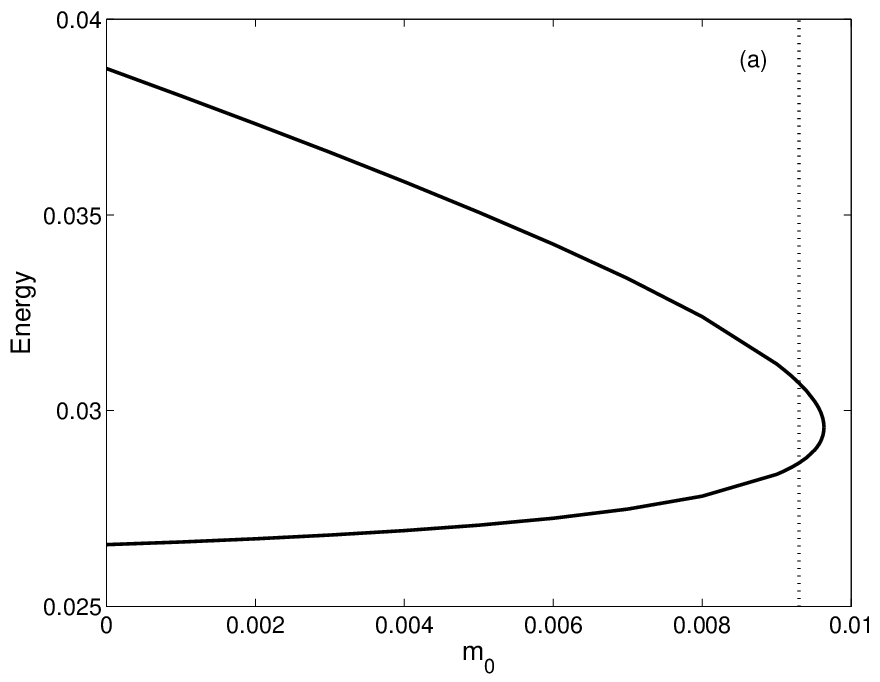

A part of the intersecting stable and unstable manifolds is shown in the left panel of figure 12. Due to their complicated windings, new intersections points appear between and as is chosen in certain windows of the parameter space, giving rise to new homoclinic solutions of (70).
An example is shown in the region marked with a rectangle (see the details in the right panel of figure 12). For some value of , a new intersection point between and appears. As is further increased, this inverse tangent bifurcation gives rise to two new homoclinic points 5’ and 6’. Correspondingly, we have numerically checked that an inverse tangent bifurcation occurs in the Klein-Gordon chain at a critical value of , giving rise to new breather solutions which do not exist in the homogeneous chain.
The point 4’ in figure 12 also exists for . Returning to figure 7, it is obtained by applying the inverse map to the point with label 2. In the homogeneous limit , this homoclinic point corresponds consequently to a two-site breather centered between and . As figure 12 shows, an increase of the mass defect moves point 5’ against point 4’ until they collide and disappear through a new tangent bifurcation. This tangent bifurcation is also numerically found in the Klein Gordon chain at critical value of the mass defect very close to the theoretical one (in both cases one obtains ).
Figure 13 shows the bifurcation diagram of the numerically computed breathers corresponding to homoclinic points 4’, 5’, 6’ (left panel), and gives their profiles for a given value of in the right panel. A numerical computation of Floquet spectra shows that all these breathers are unstable.


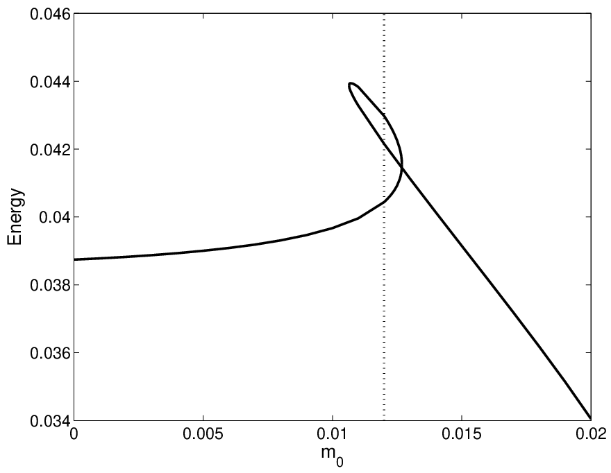

As a conclusion, we have seen that the truncated normal form (70) allows one to predict with a high precision certain breather bifurcations in the Klein-Gordon chain, which occur as the mass defect is varied. These bifurcations depend on the fine structure of the windings of the stable and unstable manifolds of the origin, computed on the truncated normal form without defect.
Acknowledgements. This work has been supported by the French Ministry of Research through the CNRS Program ACI NIM (New Interfaces of Mathematics). G.J. wishes to thank Michel Peyrard for initiating this research, and is grateful to R. MacKay for pointing out interesting bibliographical references. B.S-R. and J.C. acknowledge sponsorship by the Ministerio de Educación y Ciencia, Spain, project FIS2004-01183. B.S-R. is grateful to the Institut de Mathématiques de Toulouse (UMR 5219) where a part of this work has been carried out during a visit in Sept.-Oct. 2006.
References
- [AF88] C. Albanese and J. Fröhlich. Periodic solutions of some infinite-dimensional Hamiltonian systems associated with non-linear partial difference equations. I, Commun. Math. Phys. 116 (1988), 475-502. II, Commun. Math. Phys. 119 (1988), 677-699.
- [AF91] C. Albanese and J. Fröhlich. Perturbation theory for periodic orbits in a class of infinite-dimensional Hamiltonian systems, Commun. Math. Phys. 138 (1991), 193-205.
- [ABK04] G.L. Alfimov, V.A. Brazhnyi, V.V. Konotop. On classification of intrinsic localized modes for the discrete nonlinear Schrödinger equation, Physica D 194 (2004), 127-150.
- [And58] P.W. Anderson. Absence of diffusion in certain random lattices, Phys. Rev. 109 (1958), 1492-1505.
- [AMM99] J.F.R. Archilla, R.S. MacKay and J.L. Marin. Discrete breathers and Anderson modes : two faces of the same phenomenon ? Physica D 134 (1999), 406-418.
- [AS98] G. Arioli and A. Szulkin. Periodic motions of an infinite lattice of particles : the strongly indefinite case, Ann. Sci. Math. Québec 22 (1998), 97-119.
- [AP90] D.K. Arrowsmith and C.M. Place. An introduction to dynamical systems, Cambridge University Press, 1990.
- [AA90] S. Aubry and G. Abramovici. Chaotic trajectories in the standard map : the concept of anti-integrability, Physica D 43 (1990), 199-219.
- [Aub95] S. Aubry. Anti-integrability in dynamical and variational problems, Physica D 86 (1995), 284-296.
- [Aub98] S. Aubry. Discrete breathers in anharmonic models with acoustic phonons, Annales de l’Institut Henri Poincaré (A) Physique Théorique 68, n.4 (1998), 381-420.
- [AKK01] S. Aubry, G. Kopidakis and V. Kadelburg. Variational proof for hard discrete breathers in some classes of Hamiltonian dynamical systems, Discrete and Continuous Dynamical Systems B 1 (2001), 271-298.
- [BM03] Z. Bishnani and R.S. MacKay. Safety criteria for aperiodically forced systems, Dynamical Systems : An International Journal 18 (2003), 107-129.
- [BCKRBW00] T. Bountis, H.W. Capel, M. Kollmann, J.C. Ross, J.M. Bergamin and J.P. van der Weele. Multibreather and homoclinic orbits in 1-dimensional nonlinear lattices, Physics Letters A 268 (2000), 50-60.
- [CG98] A. Campa and A. Giansanti. Experimental tests of the Peyrard-Bishop model applied to the melting of very short DNA chains, Phys. Rev. E 58 (1998), 3585-3588.
- [CFK04] D.K. Campbell, S. Flach and Yu.S. Kivshar. Localizing Energy Through Nonlinearity and Discreteness, Physics Today, p.43-49, January 2004.
- [CGTCM06] R. Carretero-González, J.D. Talley, C. Chong and B.A. Malomed. Multistable solitons in the cubic-quintic discrete nonlinear Schrödinger equation, Physica D 216 (2006), 77-89.
- [CPAR02] J. Cuevas, F. Palmero, J.F.R. Archilla and F.R. Romero. Moving discrete breathers in a Klein-Gordon chain with an impurity, J. Phys. A: Math. Gen. 35 (2002), 10519-10530.
- [CK04] J. Cuevas and P.G. Kevrekidis. Breather statics and dynamics in Klein-Gordon chains with a bend, Phys. Rev. E 69 (2004), 056609.
- [CAR05] J. Cuevas, J.F.R. Archilla and F.R. Romero. Effect of the introduction of impurities on the stability properties of multibreathers at low coupling, Nonlinearity 18 (2005), 769-790.
- [DPB93] T. Dauxois, M. Peyrard and A.R. Bishop. Entropy-driven DNA denaturation, Phys Rev E 47, n.1 (1993), R44-R47.
- [DLHMS04] T. Dauxois, A. Litvak-Hinenzon, R.S. MacKay, A. Spanoudaki (Eds). Energy Localisation and Transfer, Advanced Series in Nonlinear Dynamics 22, World Scientific (2004).
- [EH02] J. Edler and P. Hamm. Self-trapping of the amide I band in a peptide model crystal, J. Chem. Phys. 117 (2002), 2415-2424.
- [Fla95] S. Flach. Existence of localized excitations in nonlinear Hamiltonian lattices, Phys. Rev. E 51 (1995), 1503-1507.
- [Fla96] S. Flach. Tangent bifurcation of band edge plane waves, dynamical symmetry breaking and vibrational localization, Physica D 91 (1996), 223-243.
- [FW98] S. Flach and C.R. Willis. Discrete Breathers, Physics Reports 295 (1998), 181-264.
- [FPM94] K. Forinash, M. Peyrard and B. Malomed. Interaction of discrete breathers with impurity modes, Phys Rev E 49 (1994), 3400-3411.
- [Fra74] J.M. Franks. Time dependent stable diffeomorphisms, Inventiones math. 24 (1974), 163-172.
- [FSW86] J. Fröhlich, T. Spencer and C.E. Wayne. Localization in disordered, nonlinear dynamical systems, J. Stat. Phys. 42 (1986), 247-274.
- [GLC05] B. Gershgorin, Yu.V. Lvov and David Cai. Renormalized waves and discrete breathers in -Fermi-Pasta-Ulam chains, Phys. Rev. Lett. 95 (2005), 264302.
- [GM04] J. Giannoulis and A. Mielke. The nonlinear Schrödinger equation as a macroscopic limit for an oscillator chain with cubic nonlinearities, Nonlinearity 17 (2004), 551-565.
- [GM06] J. Giannoulis and A. Mielke. Dispersive evolution of pulses in oscillator chains with general interaction potentials, Discrete and Continuous Dynamical Systems B 6 (2006), 493-523.
- [HRGB96] D. Hennig, K.Ø. Rasmussen, H. Gabriel and A. Bülow. Solitonlike solutions of the discrete nonlinear Schrödinger equation, Phys. Rev. E 54, n. 5 (1996), 5788-5801.
- [HT99] D. Hennig and G.P. Tsironis. Wave transmission in nonlinear lattices, Phys. Rep. 307 (1999), 333-432.
- [IK00] G. Iooss and K. Kirchgässner. Travelling waves in a chain of coupled nonlinear oscillators, Commun. Math. Phys. 211 (2000), 439-464.
- [Ioo00] G. Iooss. Travelling waves in the Fermi-Pasta-Ulam lattice, Nonlinearity 13 (2000), 849-866.
- [IJ05] G. Iooss and G. James. Localized waves in nonlinear oscillator chains, Chaos 15 (2005), 015113.
- [IP06] G. Iooss and D.E. Pelinovsky. Normal form for travelling kinks in discrete Klein-Gordon lattices, Physica D 216 (2006), 327-345.
- [IKSF04] M.V. Ivanchenko, O.I. Kanakov, V.D. Shalfeev and S. Flach. Discrete breathers in transient processes and thermal equilibrium, Physica D 198 (2004), 120-135.
- [Jam01] G. James. Existence of breathers on FPU lattices, C. R. Acad. Sci. Paris 332, Série I (2001), 581-586.
- [Jam03] G. James. Centre manifold reduction for quasilinear discrete systems, J. Nonlinear Sci. 13 (2003), 27-63.
- [JN04] G. James and P. Noble. Breathers on diatomic Fermi-Pasta-Ulam lattices, Physica D 196 (2004), 124-171.
- [JS05] G. James and Y. Sire. Travelling breathers with exponentially small tails in a chain of nonlinear oscillators, Commun. Math. Phys. 257 (2005), 51-85.
- [JK07] G. James and M. Kastner. Bifurcations of discrete breathers in a diatomic Fermi-Pasta-Ulam chain, Nonlinearity 20 (2007), 631-657.
- [KRBCU04] G. Kalosakas, K.Ø. Rasmussen, A.R. Bishop, C.H. Choi and A. Usheva. Sequence-specific thermal fluctuations identify start sites for DNA transcription, Europhys. Lett. 68, n. 1 (2004), 127-133.
- [Kat66] T. Kato, Perturbation theory for linear operators, Springer Verlag (1966).
- [KKK03] P.G. Kevrekidis, Yu. S. Kivshar and A.S. Kovalev. Instabilities and bifurcations of nonlinear impurity modes, Phys. Rev. E 67 (2003), 046604.
- [Kir82] K. Kirchgässner. Wave solutions of reversible systems and applications, Journal of Differential Equations 45 (1982), 113-127.
- [KBS94] S.A. Kiselev, S.R. Bickham and A.J. Sievers. Anharmonic gap mode in a one-dimensional diatomic lattice with nearest-neighbor Born-Mayer-Coulomb potentials and its interaction with a mass-defect impurity, Phys. Rev. B 50 (1994), 9135-9152.
- [KZK97] Yu. S. Kivshar, F. Zhang, A.S. Kovalev. Stable nonlinear heavy-mass impurity modes, Phys Rev B 55 (1997), 14265.
- [KA99-00] G. Kopidakis and S. Aubry. Intraband discrete breathers in disordered nonlinear systems. I. Delocalization, Physica D 130 (1999), 155-186; II. Localization, Physica D 139 (2000), 247-275.
- [MA94] R.S. MacKay and S. Aubry. Proof of existence of breathers for time-reversible or Hamiltonian networks of weakly coupled oscillators, Nonlinearity 7 (1994), 1623-1643.
- [Man06] M.E. Manley et al. Formation of a new dynamical mode in -uranium observed by inelastic X-ray and neutron scattering, Phys. Rev. Lett. 96 (2006), 125501.
- [MA96] J.L. Marin and S. Aubry. Breathers in nonlinear lattices: numerical calculation from the anticontinuous limit, Nonlinearity 9 (1996), 1501-1528.
- [Nob04] P. Noble. Existence of breathers in classical ferromagnetic lattices, Nonlinearity 17 (2004), 1-15.
- [PZ01] A. Pankov and N. Zakharchenko. On some discrete variational problems, Acta Applicandae Mathematicae 65 (2001), 295-303.
- [Pan05] A. Pankov. Travelling waves and periodic oscillations in Fermi-Pasta-Ulam lattices, Imperial College Press, London (2005).
- [PR05] D.E. Pelinovsky and V.M. Rothos. Bifurcations of travelling wave solutions in the discrete NLS equations, Physica D 202 (2005), 16-36.
- [PB89] M. Peyrard and A.R. Bishop. Statistical mechanics of a nonlinear model for DNA denaturation, Phys. Rev. Lett. 62 (1989), 2755.
- [Pey04] M. Peyrard. Nonlinear dynamics and statistical physics of DNA, Nonlinearity 17 (2004), 1-40.
- [SRJCA04] B. Sánchez-Rey, G. James, J. Cuevas and J.F.R. Archilla. Bright and dark breathers in Fermi-Pasta-Ulam lattices, Phys. Rev. B 70 (2004), 014301.
- [SS04] M. Sato and A.J. Sievers. Direct observation of the discrete character of intrinsic localized modes in an antiferromagnet, Nature 432 (2004), 486-488.
- [SES99] U.T. Schwarz, L.Q. English, and A.J. Sievers. Experimental generation and observation of intrinsic localized spin wave modes in an antiferromagnet, Phys. Rev. Lett. 83 (1999), 223-226.
- [SM97] J.A. Sepulchre and R.S. MacKay. Localized oscillations in conservative and dissipative networks of weakly coupled autonomous oscillators, Nonlinearity 10 (1997), 679-713.
- [SM98] J.A. Sepulchre and R.S. MacKay. Discrete breathers in disordered media, Physica D 113 (1998), 342-345.
- [ST88] A.J. Sievers and S. Takeno. Intrinsic localized modes in anharmonic crystals, Phys. Rev. Lett. 61 (1988), 970-973.
- [Sir05] Y. Sire. Travelling breathers in Klein-Gordon lattices as homoclinic orbits to -tori, J. Dyn. Diff. Eqs. 17 (2005), 779-823.
- [SKRC01] A.A. Sukhorukov, Yu.S. Kivshar, J.J. Rasmussen and P.L. Christiansen. Nonlinearity and disorder : classification and stability of nonlinear impurity modes, Phys. Rev. E 63 (2001), 036601.
- [Swa99] B.I. Swanson et al. Observation of intrinsically localized modes in a discrete low-dimensional material, Phys. Rev. Lett. 82 (1999), 3288-3291.
- [TP96] J.J.L. Ting and M. Peyrard. Effective breather trapping mechanism for DNA transcription, Phys Rev E 53, n.1 (1996), 1011-1020.
- [Van89] A. Vanderbauwhede. Centre manifolds, normal forms and elementary bifurcations, Dynamics Reported 2 (U. Kirchgraber and H.O. Walther, eds), John Wiley and Sons Ltd and B.G. Teubner (1989), 89-169.
- [vECLP06] Titus S. van Erp, Santiago Cuesta-Lopez, and Michel Peyrard. Bubbles and denaturation in DNA, Eur. Phys. J. E 20 (2006), 421-434.
- [VMZ03] L. Vázquez, R.S. MacKay, M.P. Zorzano (Eds). Localization and Energy Transfer in Nonlinear Systems, Proceedings of the Third Conference (San Lorenzo de El Escorial, Spain 17 - 21 June 2002), World Scientific (2003).
- [Wei99] M.I. Weinstein. Excitation thresholds for nonlinear localized modes on lattices, Nonlinearity 12 (1999), 673-691.