Evidence for a Type 1/Type 2 dichotomy in the correlation between quasar optical
polarization
and host galaxy/extended emission position anglesThanks: Table 6 is only available in electronic form at the CDS via anonymous ftp to cdsarc.u-strasbg.fr.Preprint: B. Borguet
Abstract
Aims. For Seyfert galaxies, the AGN unification model provides a simple and well established explanation of the Type 1/Type 2 dichotomy through orientation based effects. The generalization of this unification model to the higher luminosity AGNs that are the quasars remains a key question. The recent detection of Type 2 Radio-Quiet quasars seems to support such an extension. We propose to further test this scenario.
Methods. On the basis of a compilation of quasar host galaxy position angles consisting of previously published data and of new measurements performed using HST Archive images, we investigate the possible existence of a correlation between the linear polarization position angle and the host galaxy/extended emission position angle of quasars.
Results. We find that the orientation of the rest-frame UV/blue extended emission is correlated to the direction of the quasar polarization. For Type 1 quasars, the polarization is aligned with the extended UV/blue emission while these two quantities are perpendicular in Type 2 objects. This result is independent of the quasar radio-loudness. We interpret this (anti-)alignment effect in terms of scattering in a two-component polar+equatorial model which applies to both Type 1 and Type 2 objects. Moreover the orientation of the polarization –and then of the UV/blue scattered light– does not appear correlated to the major axis of the stellar component of the host galaxy measured from near-IR images.
Conclusions.
Key Words.
quasars: general – polarization1 Introduction
The study of quasars shows that we can classify them among various categories. Radio-Loud quasars (RLQ) are distinguished from the Radio-Quiet quasars (RQQ) according to their radio power (Kellerman et al. 1989 1989), and the Type 1/Type 2 objects from the presence or absence of broad emission lines in their spectrum (Lawrence 1987 1987).
One can then wonder whether there exists a common link between all these objects, i.e. are the physical processes at the origin of all quasars the same? An interesting way to tackle this question consists in the use of the linear optical polarization. Polarimetry, in combination with spectroscopy, has led to major advances in the development of a unified scheme for AGN (see Antonucci 1993 1993 for a review). The discovery of hidden broad emission lines in the polarized spectrum of the Type 2 Seyfert galaxy NGC1068 led to consider these objects as intrinsically identical to Type 1 Seyfert, the edge-on orientation of a dusty torus blocking the direct view of the central engine and the broad emission line region (Antonucci & Miller 1985 1985).
The question we investigate in this paper relates to the possible existence of a correlation between the optical polarization position angle 11 1 The polarization position angle is defined as the position angle of the maximal elongation of the electric vector in the plane of polarization, measured in degrees East of North. and the orientation of the host galaxy/extended emission 22 2 The orientation of the host galaxy is characterized by the position angle of its major axis projected onto the plane of the sky, measured in degrees East of North. in the case of RLQs and RQQs. The relation between quasars and their host galaxies may play a fundamental role in our understanding of the AGN phenomenon and in determining the importance of the feedback of AGN on their hosts.
Such a correlation has already been studied in the case of the less powerful AGN that are the Seyfert galaxies. Thompson & Martin (1988 1988) found a tendency for Seyfert 1 to have their polarization angle aligned with the major axis of their host galaxy, an observation that they interpreted as due to dichroic extinction by aligned dust grains in the Seyfert host galaxy. In the case of the more powerful AGN that are quasars, Berriman et al. (1990 1990) investigated this question. They determined by hand the of 24 PG quasars from ground based images and computed the acute angle between and . They observed that while more objects seem to appear at small values (), this effect was only marginally statistically significant.
Investigating this problem with ground based data for Type 1 quasars is hampered by the inability of separating the faint host galaxy/extended emission33 3 In the following, we use indifferently the term host galaxy or extended emission to refer to all the extended emission around the central source including stars, ionized gas or scattered light. from the blinding light of the quasar nucleus. Because of its high angular resolution and stable Point Spread Function (PSF), the Hubble Space Telescope (HST) permits to properly remove the contribution of the powerful quasar nucleus thus allowing the investigation of the host galaxy parameters. A large number of quasar host observing programs were carried out with the HST leading to a statistically useful sample of quasar host galaxy parameters (e.g. Bahcall et al. 1997 1997; Dunlop et al. 2003 2003 and many more see Sects. 2 and 3.1). Our aim is to investigate the relation on the basis of high resolution HST quasar images. We will use either position angles given in the literature or we measured ourselves from HST Archive observations (hereafter called “new data”).
The layout of this paper is as follows. In Sect. 2 we introduce the samples of quasars used in this study which possess a given in the literature. In Sect. 3, we outline the samples with good imaging data but for which no were published, and we summarize our data analysis process and the approach followed to model the HST Archive images and to derive the host galaxy parameters. In Sect.4 we briefly describe the polarization and radio data. Then in Sect. 5 we present the statistical analysis of the sample and the results obtained. In Sect. 6 we discuss the results and compare them to former studies. Finally, our conclusions are summarized in Sect. 7.
2 Description of the sample : published data
In this section we give details about the observing campaigns used in the present study excepting the new data which will be discussed in the next section. Note that our study is essentially based on intrinsically high luminosity Radio-Loud and Radio-Quiet AGN (i.e. quasars), but does not consider BLLac objects since these objects show highly variable luminosity and polarization (e.g. Urry & Padovani 1995 1995). We also select the Type 2 counterpart of Radio-Loud quasars (the Narrow Line Radio Galaxies, NLRGs, Barthel 1989 1989) from the whole RG sample on the basis of classifications given in the literature (Grandi et al. 2006 2006; Haas et al. 2005 2005; Cohen et al. 1999 1999; Rudy et al. 1983 1983; Tadhunter et al. 1998 1998; Tadhunter et al. 2002 2002; van Bemmel & Bertoldi 2001 2001; Siebenmorgen et al. 2004 2004 and Jackson & Rawlings 1997 1997).
In the following we present the samples which were analyzed in the literature and the methods used by authors to recover the host galaxy parameters from the quasar images. For more suitability in the following text, we take the convention to speak of the data of Ba97 to refer to the images/data published in the paper of Bahcall et al. (1997 1997), and so on for the other papers.
Note that in our final sample, we only consider objects from these samples if they actually possess both a reliable host position angle and an accurate enough polarization angle. So only part of the objects presented in the papers belongs to our final sample. A detailed description of the observations and measurements is available in Appendix A.1.
The visible domain :
this sample is constituted of data published in the following papers, chronologically ordered : Cimatti et al. 1993 1993, Disney et al. 1995 1995, de Koff et al. 1996 1996, Lehnert et al. 1999 1999, Martel et al. 1999 1999, Dunlop et al. 2003 2003, Floyd et al. 2004 2004 and McLure et al. 2004 2004, respectively abbreviated Ci93, Di95, Dk96, Le99, Ma99, Du03, Fl04 and Mc04.
The radio galaxy and quasar images studied in these papers were mostly (except the RGs from Ci93) imaged through an R-band filter with the HST WFPC2 camera. The sample spans a redshift range from 0.0 to 2.0 and is essentially made out of 3CR and PG objects. Considering these samples, we obtain a final number of 79 objects possessing a published in the visible domain together with a polarization position angle.
The near-IR domain :
the near-IR compilation contains several samples coming from surveys using the NICMOS HST camera or ground based images. All the targets of the resulting sample were observed in the near-IR using K and H-band filters. The host galaxy data were retrieved from the papers of Taylor et al. 1996 1996, Percival et al. 2001 2001, Guyon et al. 2006 2006 and Veilleux et al. 2006 2006 abbreviated respectively Ta96, Pe01, Gu06 and Ve06. The compiled resulting sample, considering only the objects for which we have at least a and a polarization position angle contains 21 objects with redshifts .
Determination of the :
the published in the aforementioned papers were measured as follows. The first step to determine the position angle of a quasar host galaxy is the proper subtraction of the bright central source which dominates the optical emission of Type 1 objects. To this aim, a careful PSF construction is realized in order to precisely characterize the profile of a point like source imaged by a given instrument. This PSF is then scaled to the quasar intensity and subtracted from the quasar image allowing in most cases the detection of the underlying host. This first step is realized for all quasars except for Type 2 objects in which the heavy obscuration of the central source provides a non-contaminated view of the host.
Several techniques are then used to derive the host parameters ( and ) either ellipse fitting on the host image followed by the measurement of the model position angle at a chosen surface brightness, or two-dimensional galaxy profile fitting over the nucleus-subtracted image. These techniques give rather similar results since the crucial step remains the proper separation between the point-like component and the underlying host.
3 Measurements of new
3.1 The samples
The samples are constituted of available quasar/RG HST observations retrieved from the Archive, but for which the images and more particularly the host galaxy parameters were not thoroughly studied or published in the literature. Detailed observational properties of these samples are available in Appendix A.2, while major properties are summarized in Table 1.
The visible domain :
this sample gathers quasars imaged in the V to R-band using the HST WFPC2 or ACS camera. The total sample consists of 53 objects coming from the following papers: Bahcall et al. 1997 1997, Boyce et al. 1998 1998, Marble et al. 2003 2003 and Zakamska et al. 2006 2006 hereafter abbreviated Ba97, Bo98, Ma03 and Za06 respectively. This sample essentially contains 3CR, 2-Micron All Sky Survey (2MASS), Sloan Digital Sky Survey (SDSS) and PG quasars.
The near-IR domain :
3.2 The method
Here we describe the method we used to derive host galaxy position angle and axial ratio from the images. First we outline the images reduction steps and then we give an overview of the technique used to disentangle the quasar nuclear and host galaxy contributions. We then present the construction of the Point Spread Function (PSF) necessary for an accurate separation. The results of the modelling are finally given and compared to the results of other studies in the following subsection.
| Reference44 4 Reference to the paper where the images were published. | Prop ID55 5 Corresponding HST Proposal ID. | Instrument66 6 Name of the camera. | Filter77 7 Name of the filter used. |
|---|---|---|---|
| Ba97 | 5343,5099 | WFPC2-WF3 | F606M |
| Bo98 | 6303,5143 | WFPC2-PC1 | F702M |
| Ml01 | 7421 | NICMOS-NIC2 | F160M |
| Ku01 | 7447 | NICMOS-NIC1 | F110M&F165M |
| Ma03 | 9057 | WFPC2-PC1 | F814M |
| Za06 | 9905 | ACS-WFC | F550M |
3.2.1 Image reduction
The quasar images were retrieved from the MAST HST Archive of the Space Telescope Science Institute (STScI, http://archive.stsci.edu/astro). All the images are already pre-processed by standard STSDAS pipeline softwares adapted to each HST instrument. This pre-processing essentially consists in dark frame and bias substraction along with flat-fielding, with the best reference files available. In the case of the ACS images, where the geometric distortion in the WFC camera is significant, an additional step was added to correct these distortions thanks to the routine (Koekemoer et al. 2002 2002).
In addition to this pre-processing, we carried out two additional processing steps. The first consists in the removal of cosmic rays using the task of the Image Reduction and Analysis Facility (IRAF) software which rejects high pixels from sets of exposures of the same field in an iterative way. These bad pixels are not used in the creation of the output image providing a final cosmic ray free image. In the case of the NICMOS data, this step is not essential since the MULTIACCUM mode used in the image acquisition phase already realizes this processing when acquiring the data (Schultz et al. 2005 2005).
The second step consists in the background subtraction. As the backgrounds on the WFPC2 and ACS WFC camera are extremely flat around the targets of interest we simply estimated the mean of the background level in each image from several subset of pixels excluding obvious sources, and then subtracted this mean value to each pixel of the image. In the case of the NICMOS data, the known pedestal effect (variable quadrant bias of the detectors) was not taken into account since the objects images were always almost centered in one of the quadrants.
3.2.2 Image processing
As our primarily aim is to determine the position angle of the host galaxy surrounding nuclear dominated objects, we have to distinguish the faint fuzz of the galaxy from the quasar. The use of high resolution HST images partly solves this problem, but rises another one : the complex path of the light rays in the instrument create a complex PSF with quite extended wings that can cover, scaled to the intensity of the quasar, the underlying galaxy. The use of a deconvolution technique makes it possible to separate quite efficiently the light of the point like quasar central source (roughly a scaled PSF) from the light of the host. We used a version of the MCS algorithm (Magain et al. 1998 1998) that is well suited to deconvolve the HST images while adjusting an analytical galaxy model.
Our image processing proceeds in essentially two steps. In the first stage, the parameters (intensity and position) of the point source are adjusted to subtract the contribution of the quasar. This contribution is estimated so that a minimal amount of PSF structure remains in the image. This step has to be realized with particular care as the inner pixels (out to a radius of 5 pixels for the extreme cases) of the quasar image may be saturated, so that the PSF subtraction process may become quite subjective.
The second stage corresponds to the fitting of an analytical galaxy profile (properly convolved with the HST PSF) to the PSF subtracted images. The analytic profile we used consists in a typical Sérsic (Sérsic 1968 1968) profile:
| (1) |
where stands for the central surface brightness, and describes its profile (the profile is called elliptical or de Vaucouleurs if and spiral or disk-like if ). A coordinate change allows us to recover the axial ratio () and the position angle () of the model fitted to the data. Since we are essentially interested in the orientation of the major light concentration, we only use in the following a de Vaucouleurs profile, noting after some tests that does not strongly depend on .
3.2.3 PSF creation
The quality of the image processing critically depends on the accuracy of the PSF used. A careful construction of the PSF is of prime importance to properly separate the contribution of the bright nucleus from that of the host galaxy. In the MCS method adapted to HST images, the construction of the PSF proceeds in two steps. The first step consists in the fitting of a sub-sampled numerical estimate of the PSF computed with the TinyTim package (Krist & Hook 2004 2004) to an original resolution one (also estimated with TinyTim). This step provides the Tinydec i.e. a PSF that has a better resolution than the observed one. The second step consists in a second fit, where the Tinydec is fitted to an observed PSF (typically a calibration star lying in a weakly crowded field) in order to improve the agreement between the numerical estimate and the observed point source. This second fit is important since the TinyTim package is unable to give an accurate estimation of the external fainter halo () as well as of the diffraction spikes (McLure et al. 2000 2000; Pian et al. 2002 2002).
Usually one or more stars were imaged during each of the considered campaigns with growing exposures times, allowing the construction of a deep unsaturated PSF star. The aforementioned procedure could not be used in the case of the Ma03 and Za06 campaigns since no time was devoted to the observation of a specific PSF star, then forcing us to use the Tinydec as the PSF. However the lack of observed standard PSF star is less constraining in these two cases since the quasars imaged are generally heavily obscured objects such that the central source contribution and the intensity of the associated scattered halo are weak (or null for the Type 2 objects of Za06).
3.2.4 The error frame
In order to determine whether a given quasar model provides an accurate description of an observed image, a minimization is used by the MCS program :
| (2) |
where represents the reduced quasar image, the quasar model, and the standard deviation in the corresponding pixel (called the error frame). A careful construction of the error frame is mandatory for each image in order to avoid biased results.
The error term accounts for different elements : first, for a Poissonian component due to photon shot noise and dark current as well as the noise induced by the CCD readout. The second component accounts for the detector pixels that are known to work badly, these pixels being indexed in flag frames available via the STScI website. We used this frame to construct masks such that zero weight (i.e. ) is allocated to these indexed pixels while this value is set to one everywhere else over the frame. The last component accounts for saturated regions in the observed image due to the long exposure time required for the imaging of the faint host galaxies. We accounted for this final component by assigning a null weight to the implied pixels. These masks are then multiplied by the original constructed in the first step.
3.3 The resulting
The results of our image analysis are summarized in Table 6. Columns are as follows : (1) object name, (2) redshift of the object, (3) radio-loudness of the object (RL or RQ), (4) source of the image, (5) spectral domain of the image (visible (Vis) or near-IR (NIR)), (6) type of the host galaxy (E : elliptical, S : spiral and U : undefined), (7) and (8) axial ratio and position angle of the host ( in degrees, East of North) and (9) a quality criterion (1, 2 or 3, with 1 being the highest quality). The parameters in Col. (6) and Col. (9) are defined in the following subsections.
Fig. 1 illustrates the results for two representative objects of our new data sample. From left to right, we show for each object the final reduced HST image, a closer view on the PSF-subtracted image, the host galaxy model fitted over the PSF-subtracted image and the model-subtracted residual image (darker regions account for un-modelled details such as spiral arms, interaction features etc.).


3.3.1 Morphology of the host
As we use only a de Vaucouleurs model to derive the host galaxy parameters, we can not provide a host morphology classification on the basis of a better description of the host by a spheroidal or a disc-like profile. The morphological classification was thus realized by careful visual inspection of both the PSF-subtracted image and the model-subtracted residual image. We adopt a classification scheme similar to the one defined in Guyon et al. (2006 2006) : if a bar or spiral arms are obvious in one image, the host is classified as a Spiral (disk-present) and abbreviated by S in Table 6. If no spiral structure or bar are visible in the image, we classify the host as an Elliptical galaxy (E). The remaining host galaxies (those presenting strong interaction traces/complex morphology, multiple nuclei, etc.) were assigned to the “undefined” class (abbreviated U). Finally, in some cases no host galaxy was detected even after PSF-subtraction, essentially due to the comparatively high redshift or to the insensitivity to low surface brightness features due to short exposure times.
3.3.2 Reliability and error estimates
The and reported in Table 6 are determined within uncertainties that essentially come from the degeneracy existing between the host galaxy model and the estimated nuclear contribution. These uncertainties are quite difficult to estimate, especially in our case where the objects come from samples with different observational circumstances.
A useful test to estimate the uncertainties of the derived parameters was proposed in Fl04 : to ensure that the modelling routines of the host reach the global minimum within the six-dimensional model parameter space, they used six different starting point for each object close to the best-fitting parameter value. Using the same method, we checked the quality of the determination of the host parameters by starting the MCS host modelling routine with initial parameters which progressively departs from the parameter set we found during the first modelling of each object. This enabled us to also check the stability of the solution found.
This procedure allowed us to distinguish three cases that we relate to a quality criterion (Col. (9) in Table 6). The first, called 1, accounts for situations where the modelling algorithm converges towards similar solutions whatever the starting point used, then giving reliable host parameters. The second, noted 2, corresponds to the cases where the solution strongly depends upon the initial parameters (generally corresponding to the faintest/rounder hosts). The last one, noted 3, is attributed to the cases where we detect no host galaxy after the PSF-subtraction step.
Moreover, we have also considered among our sample of new data five objects which already had a determined in the literature. We find a good agreement88 8 We find within for the class 1 quality objects, see Appendix B for more details. between the previously published parameters and the one we derived, assessing the capability of the method used in our study to recover host galaxy parameters. This is not a surprise since the crucial step in the determination essentially lies in the proper subtraction of the quasar nucleus, a step which is carefully carried out for each of the objects of our compilation (see Sect. 2). Finally we also carried out simple ellipse fitting on the nuclear-subtracted images and we observed that the derived agree (within ) with those derived using the 2D profile fitting procedure described in Sect. 3.2.2. On the other hand the axial ratio is more sensitive to the PSF subtraction and then not reliable enough to be used in the study. Therefore, in the following, we only use to cut the sample (cf. Sect. 5).
4 Polarimetric and radio data
4.1 The polarimetric data
Most polarimetric data (the degree of polarization and the polarization angle ) are taken from a compilation of measurements from the literature (Hutsemékers et al. 2005 2005). The polarimetric measurements for the objects of the sample of Za06 were published in their paper. For the 2-MASS reddened objects of the Ma03 sample, the polarimetric data are taken from Smith et al. (2002 2002).
From this compilation we only considered and used data for objects where significant polarization is detected (i.e. such that ). This also ensures that we only select data for which the the polarization angle is known with an uncertainty of .
| Name | Catalog Name | 99 9 measured in degrees East of North. | Ref.1010 10 References. (1) Bridle et al. 1994 1994; (2) Price et al. 1993 1993; (3) Bogers et al. 1994 1994; (4) Reid et al. 1995 1995; (5) Lister et al. 1994 1994; (6) Hintzen et al. 1983 1983; (7) Gower & Hutchings 1984a; (8) Owen & Pushell 1984 1984; (9) Gower & Hutchings 1984b; (10) Readhead et al. 1979 1979. | |
| (B1950) | () | |||
| 0133+207 | 3C 47.0 | 0.425 | 35 | Le99 |
| 0137+012 | 4C 01.04 | 0.258 | 30 | 5,6,7 |
| 0340+048 | 3C 393.0 | 0.357 | 40 | Le99 |
| 0518+165 | 3C 138.0 | 0.759 | 70 | Le99 |
| 0538+498 | 3C 147.0 | 0.545 | 60 | Le99 |
| 0710+118 | 3C 175.0 | 0.770 | 60 | Le99 |
| 0723+679 | 3C 179.0 | 0.846 | 90 | Le99 |
| 0740+380 | 3C 186.0 | 1.067 | 140 | Le99 |
| 0758+143 | 3C 190.0 | 1.195 | 30 | Le99 |
| 0906+430 | 3C 216.0 | 0.670 | 40 | Le99 |
| 1020– 103 | … | 0.197 | 155 | 5,9 |
| 1100+772 | 3C 249.1 | 0.311 | 100 | Le99 |
| 1111+408 | 3C 254.0 | 0.736 | 110 | Le99 |
| 1137+660 | 3C 263.0 | 0.646 | 110 | Le99 |
| 1150+497 | 4C 49.22 | 0.334 | 15 | 4,8 |
| 1226+023 | 3C 273.0 | 0.158 | 60 | 10 |
| 1250+568 | 3C 277.1 | 0.320 | 130 | Le99 |
| 1302– 102 | … | 0.286 | 25 | 10 |
| 1416+067 | 3C 298.0 | 1.436 | 90 | Le99 |
| 1458+718 | 3C 309.1 | 0.905 | 145 | Le99 |
| 1545+210 | 3C 323.1 | 0.266 | 20 | 3,9 |
| 1618+177 | 3C 334.0 | 0.555 | 140 | Le99 |
| 1704+608 | 3C 351.0 | 0.371 | 40 | 1,2,4 |
| 1828+487 | 3C 380.0 | 0.692 | 135 | Le99 |
| 2120+168 | 3C 432.0 | 1.785 | 135 | Le99 |
| 2135– 147 | … | 0.200 | 100 | 9 |
| 2247+140 | 4C 14.82 | 0.237 | 35 | 5 |
4.2 The radio data
For each of the objects from of our compilation which possess a and a , we searched in the literature for radio data. The radio data, referring to the RLQs, consists of radio-jet position angles determined on the basis of published Very Large Array (VLA) maps from the literature. The position angle refers to the orientation defined by the axis of the prominent jet (when seen), otherwise it is the position angle of the large scale radio morphology (brightest hotspot, outer lobes) relative to the core. As for the optical and near-IR , the angles are computed in degrees East of North.
A large part of the Type 1 RLQ radio data comes from the measurements realized by Le99. Other Type 1 RLQ radio-jet data were found in the literature for several quasars (Table 3). In the case of the Type 2 RLQs, the data come from the papers of Ci93, Dk96 and Ma99 and essentially consist in compilations of VLA/Multi Element Radio Linked Interferometer Network (MERLIN) surveys measurements from the literature.
5 Search for correlations
The Table 6 with all data is available on-line. For the analysis, we select the objects for which the data are relevant and accurate. Let us quickly summarize the criteria we use.
- 1.
We do not consider Seyfert galaxies in this study. To avoid these objects, we only consider objects with in the Véron catalogue version 12 (Véron-Cetty & Véron 2006 2006). Two objects (0204+292 (Du03, = -22.4) and 2344+184 (Du03, = -22.0)) are then excluded from our sample. Two objects at the borderline (1635+119 (Du03, -22.8) and 0906+430 (Le99, =-22.9)) are kept. This criterion can not be crudely applied to the reddened objets of Ma03 and the Type 2 Radio-Quiet objects of Za06 since the luminosity of those objects is attenuated in the -band. However, their high luminosity in the -band or in the [O iii] emission lines testifies their membership to the intrinsically luminous quasar sample.
- 2.
We decided to fix an axial ratio limit in order to eliminate the roundest host galaxy morphology for which no accurate determination could be obtained.
- 3.
When several data were available for a given object parameter, we always selected the value with the smallest uncertainty.
- 4.
For consistency, we always preferred data coming from larger homogeneous samples to those selected from smaller ones.
| Selected Sample1111 11 Criteria used to define sub-samples. | 1212 12 Size of the selected Type 1 subsample. | 1313 13 Size of the selected Type 2 subsample. | 1414 14 Probability (in percent) that the of Type 1 and Type 2 objects are selected from the same parent sample. |
| (%) | |||
| RQ | 24 | 5 | 7.24 |
| RQ () | 15 | 5 | 15.75 |
| RQ () | 8 | 5 | 0.11 |
| RQ () | 5 | 5 | 0.37 |
| RL | 16 | 16 | 2.30 |
| RL () | 14 | 15 | 1.95 |
| RL () | 13 | 10 | 0.23 |
| RL () | 13 | 10 | 0.23 |
| RQ+RL | 40 | 21 | 0.24 |
| RQ+RL () | 29 | 20 | 0.21 |
| RQ+RL () | 21 | 15 | 0.01 |
| RQ+RL () | 18 | 15 | 0.03 |


5.1 The - correlation
Here we consider the host galaxy data that were derived using observations taken in the visible domain ( Å). The data obtained in the near-IR are discussed at the end of this section. We define as the acute angle between the polarization position angle and the host galaxy orientation in the visible : . Its value is defined between 0 and 90 degrees.
5.1.1 The Radio-quiet objects
The upper panel of Fig. 2 summarizes the behavior as a function of the redshift for both Type 1 and Type 2 RQQ objects in our sample. While at small redshifts there seems to be no clear correlation between and for Type 1 objects (the redshift extent of the Type 2 RQQ sample is too limited to conclude), a distinct separation between the Type 1 and Type 2 behavior is noted for objects lying at larger redshifts () where the polarization position angle of Type 1 objects is preferentially parallel to the host major axis (“alignment” : ) while the polarization is mostly perpendicular to the host major axis in Type 2 quasars (“anti-alignment” : ). We also observe this type of behavior if we only consider the more polarized objects ( pictured by filled symbols). It is worth noting that the 2MASS reddened quasars from the Ma03 study appear preferentially at small values () as other un-reddened Type 1 objects from the sample. We finally note that one Type 2 RQQ quasar at appears at small . The behavior of this object, SDSS J0920+4531, already discussed in Za06, seems to be due to an unfortunate apparent superposition of a close companion galaxy leading to a biased determination.
In order to assess the significance of the alignment observed in the upper panel of Fig. 2 we carried out statistical tests on the Type 1 and Type 2 RQQ samples. We used the two sample non-parametric Kolmogorov-Smirnov (-) test to determine if the Type 1 and Type 2 distributions are drawn from the same parent population. The results of the - tests applied to the two aforementioned samples using several selection criteria are summarized in Table 4. From these results, we can note that, while accounting for the whole RQQ sample does not allow an effective distinction between the Type 1 and Type 2 parent sample, the selection of the higher redshift objects () shows that the probability that the difference in the behavior seen among the two samples is fortuitous is of only 0.11 %. The same conclusions can be reached if we only consider the more polarized objects () but with a weaker statistical significance as the selected sample becomes smaller.
We also investigated the variation of as a function of the redshift considering Type 1 and Type 2 objects separately. To this aim, we performed a non parametric Kendall- rank test on the Type 1 RQQ sample in order to check the strength of the correlation between the alignment () and the redshift. This statistical test uses the relative order of ranks in a data set to determine the likelihood of a correlation. We found a 4% probability that the anti-correlation between the and the redshift is purely fortuitous in the case of the Type 1 RQQ sample. We do not carry this test on our Type 2 RQQ sample given its limited redshift range.
5.1.2 The Radio-loud objects
The relation is also studied in the case of the Radio-Loud sample. The lower panel of Fig. 2 illustrates the observed behavior in this case. Once again, the distribution is clearly non-random. A first look allows to see that the Type 1 RLQs are preferentially found at small (i.e. alignment between the polarization angle and the major axis of the host). Type 2 objects often exhibit large offset angles, , indicating an anti-alignment between the polarization angle and the host galaxy position angle (Cimatti et al. 1993 1993).
The lower panel of Fig. 2 suggests a dependence of as a function of the redshift as already noted for the Type 2 RLQs (Cimatti et al. 1993 1993). Indeed, at small redshift (), as in the Radio-Quiet case (upper panel of Fig. 2), we do not find any particular difference for either Type 1 or Type 2 objects while at higher redshift () we observe a clear separation of the .
Statistical tests were carried out on the data in order to assess the strength of the (anti-)alignment. The results of a two sample - test using several selection criteria applied to Radio-Loud objects are summarized in Table 4. The two sample - test comparing the distribution of Type 1 and Type 2 on the whole RLQ sample shows that there is only a 2.3% probability that the of the two samples are selected from the same parent distribution. More selective criteria1515 15 Although the alignment/anti-alignment seems to appear at higher redshift for RLQs, we keep the cutoff in the test at for consistency with RQQs. However, using a higher redshift cutoff results in even more significant correlations. (, or both) on the RLQ sample reinforce the conclusion of the statistical test.
A Kendall- correlation test considering Type 1 and Type 2 objects separately was applied to the sample in order to investigate the redshift dependency of the distribution. For the Type 1 RLQs, the result of the test shows that there is a 4% probability that the anti-correlation of the with the redshift is purely fortuitous while for Type 2 objects the probability that the correlation is fortuitous is only of 0.2%.
5.1.3 A global view
A global look at both panels of Fig. 2 suggests a similar behavior of the Type 1/Type 2 quasars whatever their radio-loudness: at the Type 1 objects systematically lie at small having their polarization mainly parallel () to their morphological major axis while the Type 2 objects are found at higher offset angle (). These observations are supported by statistical tests carried out on the mixed RQQ and RLQ sample (Table 4). The Kendall- correlation test lead to the conclusion that there is a 0.2 % probability that the correlation between and is purely fortuitous for the Type 2 quasars and of 0.4 % that the anti-correlation is fortuitous for Type 1 objects.
In order to verify that the difference in the behavior of between Type 1 and Type 2 quasars actually corresponds to alignment and anti-alignment respectively, we computed the mean value of the for both samples at separately and compared this value to the distribution of mean offset angles computed from simulated samples obtained by shuffling the among the objects. We found that the (resp. ) value measured for the Type 1 (resp. Type 2) quasars has a probability of 0.3 % (resp. 0.02 %) to occur in a random distribution of polarization and host position angles. This test was not applied to RQQ and RLQ samples separately given the small number of objects.
We also investigated the - correlation for the RQQ and RLQ samples using the compilation of near-IR data. However for those data, we do not see any clear correlations between the polarization angle and the host galaxy position angle even at higher redshifts (). This lack of correlation was confirmed by the - and Kendall- tests.
5.2 Other interesting correlations

5.2.1 The - correlation
Using the available VLA radio-jet orientation for the Radio-Loud objects of our sample possessing optical polarization measurements (Table 3 and Ci93), we also investigate the - correlation. We define the radio-jet/polarization offset angle in the same way as the offset defined in Sect. 5.1: whose value is comprised between 0 and 90 degrees.
Fig. 3 synthesizes the distribution for the Radio-Loud objects as a function of the redshift. One can note that the radio-jet of Type 1 Radio-Loud quasars are mostly aligned with the polarization () while these two directions are mostly anti-aligned in Type 2 objects (). Moreover, we do not see any redshift dependence of the correlation. We carry out - test over the distribution of Type 1 and Type 2 objects. The two sample - test shows that there is less than a 0.001 % probability that both samples are selected from the same parent distribution. This result is even more significant if we only consider the % quasars. We also find a 0.17 % (resp. 0.06 %) probability that the measured for Type 1 RLQs (resp. for Type 2) comes from a random distribution.
These (anti-)alignment effects were already reported previously in the literature. For the Type 1 objects, a clearly non-random distribution of has been reported by many authors (e.g. Stockman et al. 1979 1979; Rusk & Seaquist 1985 1985; Berriman et al. 1990 1990; Lister & Smith 2000 2000), showing that the optical polarization angle of Type 1 RLQs mostly aligns with their radio-morphology. For the Type 2 Radio-Loud quasars the anti-alignment between the radio-jets and the optical polarization is known as part of the so called “RG alignment effect” observed in high- radio galaxies (e.g. McCarthy et al. (1987 1987); Chambers et al. (1987 1987); Cimatti et al. (1993 1993)). Indeed, using polarization measurements and VLA radio observations of RGs, they found a strong anti-alignment between the linear polarization orientation and the radio structure.

5.2.2 The - correlation
Using the radio-jet orientations given in Table 3 and Ci93 for the Radio-Loud objects of our sample with a reliable host galaxy position angle, we finally look at the correlation of the radio-jet with the morphology of the host. We define the offset angle between the radio-jet and host major axis position angle using the same definition as in the preceding sections. Fig. 4 summarizes the behavior of as a function of the redshift.
For the Type 1 RLQs, we note a significant alignment ( that the measured is due to chance) between the host galaxy’s main orientation and the radio-jet orientation, as first reported within a larger sample in Le99. This is not a surprise since of the Type 1 RLQ sample used to check this correlation is made of the measurements given in Le99.
For the Type 2 RLQs (the NLRGs) we also note an alignment () between the radio-jet and the host position angle. The permutation test gives a that the measured is due to chance. Although one might suspect a redshift dependence on Fig. 4, it is not significant in our sample (as the result of the Kendall- test). Let us notice that this alignment is known as part of the “RG alignment effect” (e.g. McCarthy et al. (1987 1987); Chambers et al. (1987 1987)) where the optical morphology of higher redshift () RGs aligns with the radio-jet.
| Radio Type | Correlation | Type 11616 16 Numbers in parentheses give the reference to the first detection of a given correlation for Type 1 and Type 2 quasars : Chambers et al. 1987 1987; McCarthy et al. 1987 1987; Cimatti et al. 1993 1993; Le99; (3) Stockman et al. 1979 1979; (4) Biretta et al. 2002 2002; (5) Zakamska et al. 2006 2006 and (6) this work. | Type 2a |
|---|---|---|---|
| Radio-Quiet | |||
| Radio-Loud | |||
| Radio-Loud | |||
| Radio-Loud |
5.3 Summary of the results
The known correlations between quasar orientation parameters are summarized in Table 5. The main result of our study is the discovery of a correlation between and in quasars observed whatever their radio-loudness but depending on the spectroscopic type of the source. We find that while high redshift Type 2 quasars exhibit an anti-alignment of their optical polarization angle with their optical, rest frame UV/blue, morphology, the optical host galaxy position angle is preferentially aligned with the polarization angle in Type 1 quasars.
Another interesting result is the redshift dependence of the alignment. Indeed, as suggested by both upper and lower panels of Fig. 2 and the results of the statistical tests, the alignment becomes significant if we consider redshifts higher than for either Radio-Loud or Radio-Quiet objects. This observation may explain the lack of correlation observed by Berriman et al. (1990 1990) between and since the redshift extent of their sample was rather small (among their 24 objects with , only 5 of them have ). Note that the precise cutoff is not clearly determined and might be slightly higher as suggested by RLQs (Fig. 2). Observations of RQQs at higher would be needed to clarify this point.
Finally, we note that, while the alignment between the host galaxy position angle and the polarization angle is clearly observed and statistically significant in the case of the optical data, we do not find a similar behavior with the near-IR data. Optical and K-band studies of high RGs already showed that while an alignment effect is observed between their optical emission and their radio axis, a significantly weaker alignment is observed between the K-band emission and the radio axis (Rigler et al. 1992 1992; Dunlop & Peacock 1993 1993; Best et al. 1998 1998). This argues in favor of a scheme where the K-band emission is not necessarily related to the visible (rest-frame blue) light.
6 Discussion
6.1 The observed correlation

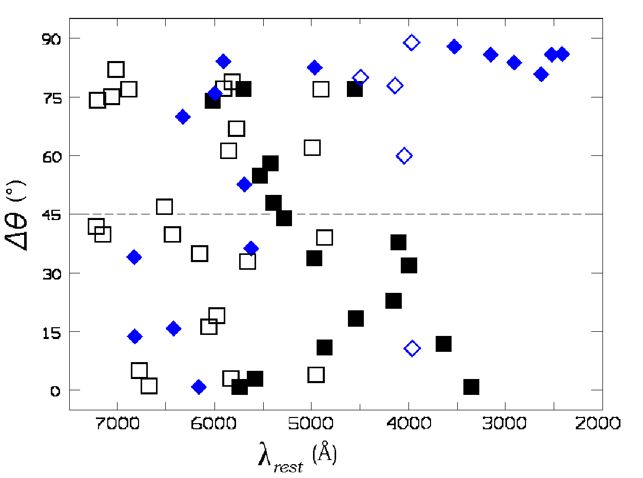
In Sect. 5 we reported on the existence of an (anti-)alignment between the linear polarization and the host galaxy position angle of (Type 2) Type 1 quasars. We noticed that this behavior seems to be independent of the radio-loudness. It is also interesting to remind the lack of correlation in the near-IR domain and the redshift dependence of the (anti-)alignment. These last two facts lead us to think that the observed correlations might be linked to the rest-frame UV/blue part of the quasar light which is redshifted to optical wavelengths for the higher objects. This hypothesis is supported by Fig. 5, where we plot as a function of , the rest-frame wavelength at which is measured (i.e. the central wavelength of the imaging filter divided by ).
We note that while at longer wavelengths there is no particular behavior in the distribution for either Type 1 or Type 2 objects, the (anti-)alignment effect clearly appears at shorter wavelengths ( Å). At Å, a two sample - test shows that there is a 0.01 % probability that the distribution of Type 1 and Type 2 quasars is drawn from the same parent sample.
6.2 The UV/blue continuum and the origin of the correlation
The morphology of Type 2 Radio-Loud objects (NLRGs) has been extensively studied in the literature since those objects do not possess a bright central nucleus masking the underlying host and can be observed at high redshifts. Imaged at optical wavelengths, higher redshift RGs () are known to show the aforementioned “RG alignment effect” where the extended rest frame UV/blue continuum emission aligns with the radio-jet. This alignment, not seen in the near-IR images of the same objects (Rigler et al. 1992 1992) leads to a two component RG model: at shorter wavelengths, the continuum is dominated by an extended UV/blue component aligned with the radio axis while at longer wavelengths, the quasar light is dominated by a stellar component which possesses the morphology and physical dimensions of elliptical galaxies.
This extended UV/blue continuum which can show a quite complex morphology (McCarthy et al. 1997 1997) was primarily interpreted, given its alignment with the radio-jet, as massive star formation regions triggered by the shocks associated to the passage of the radio-jet through the host galaxy (McCarthy et al. 1987 1987). However, as we briefly recalled in Sect. 5.1.2, high redshift NLRGs are also known to show an anti-alignment between their optical linear polarization and their rest frame UV/blue morphological structure (e.g. Cimatti et al. 1993 1993; Hurt et al. 1999 1999), supporting the possibility that at least part of this extended UV/blue light is due to the polar scattering of the light from the quasar nucleus by electrons and/or dust (di Serego Alighieri et al. 1989 1989; Cimatti et al. 1993 1993; di Serego Alighieri et al. 1993 1993; Dey et al. 1996 1996; Tadhunter et al. 2002 2002). Indeed, this assumption provides a simple explanation to the fact that the polarization angle is perpendicular to the optical, extended rest frame UV/blue light in the host galaxy.
Due to their apparent faintness and the absence of strong radio counterpart, Type 2 Radio-Quiet quasars have long been searched for. The hard X-ray and SDSS surveys recently unveiled large samples of Type 2 RQQ candidates, showing that these objects are not extraordinarily rare (e.g. Zakamska et al. 2003 2003 and references therein). The HST spectropolarimetric study of a sample of 12 Type 2 RQQs revealed that a large part of them (9 out of 12) possess high optical polarization and that for 5 objects their polarized spectra contain broad emission lines betraying the presence of a Type 1 nucleus (Zakamska et al. 2005 2005). Three band HST imaging of 9 Type 2 RQQs also reveals some morphologically complex emission which appears in the bluer images (Za06). These structures were interpreted as scattering cones since their position angle lies almost perpendicularly to the - polarization plane. As in NLRGs, scattering in the extended UV/blue component seems to represent a viable interpretation of the origin of the detected polarization.
The detection of a hypothetical extended blue component in either Radio-Loud or Radio-Quiet Type 1 quasars is hindered by the central source whose strong contribution at smaller wavelengths remains difficult to estimate and properly subtract. However, if Type 1 and Type 2 objects are, according to the unification model, intrinsically identical, the extended scattering region resolved in Type 2 quasars should also be present, but masked by the higher apparent brightness of the unobscured central source. Since the viewing angle of Type 1 and Type 2 objects is thought to be an essential parameter controlling the observed properties of those objects, the polarization geometry may also be affected by the viewing angle. While in this framework Type 2 objects are almost seen edge-on such that the extended polar scattering regions produce a polarization angle perpendicular to the symmetry axis of the AGN (pictured by the radio-jet axis in the RLQ objects), the situation may be different in the nearly face-on Type 1 quasars.
An enticing interpretation of the polarization properties was recently proposed for the Seyfert galaxies. Indeed, Seyfert galaxies exhibit some kind of alignment effect between their optical linear polarization and their radio axis. While the Type 2 objects polarization is known to be anti-aligned with the radio axis (Antonucci 1983 1983), the polarization originating from scattering cones perpendicular to the obscuring torus (Antonucci & Miller 1985 1985), Type 1 Seyferts are found to be of both kinds (aligned and anti-aligned, Smith et al. 2002 2002). The scenario proposed to account for these observations consists of a two component polar+equatorial scattering model (Smith et al. 2004 2004, 2005 2005; Goosmann et al. 2007 2007). While the extended polar scattering region accounts for the perpendicular polarization, the much smaller equatorial disk-like component inside the obscuring torus produces a polarization which, projected onto the plane of the sky, is parallel to the symmetry axis of the system (see Fig. 6). In this framework, Type 2 polarization properties are dominated by polar scattering, the equatorial component being hidden by the dusty torus. In Type 1 objects, the smaller but significantly non-zero inclination angle of the system is such that both scattering regions contribute to the polarized flux, the resulting polarization being dominated by the equatorial scattering component (Smith et al. 2002 2002).

This two component scattering scheme seems to nicely fit our observations as it provides an explanation to the correlations found in Sect. 5.1 assuming that the observed polarization is due to scattering (in both RQ and RL objects) and that the morphology of the host galaxy/extended emission observed in higher redshift quasars is, at least in part, related to scattered UV/blue light1717 17 Let us emphasize that only the polar scattering region –assumed to be parallel to the symmetry axis of the system– can be angularly resolved (in principle in both Type 1 and Type 2 objects). The equatorial scattering region -perpendicular to the symmetry axis- is too small to be resolved. Note that in this framework, given the projections effects and the presence of two competing scattering regions, we expect the dispersion of the to be higher for Type 1 quasars than for Type 2 ones as it might be suspected in Fig. 2.. The model also provides a simple explanation of the alignment seen in Type 1 and Type 2 Radio-Loud quasars between their polarization position angle and their radio jets since the radio-jets are thought to be emitted along the symmetry axis of the accretion disk which also defines the direction of the extension of the polar scattering regions. Moreover, assuming the proposed model applies and reminding the lack of correlation in the near-IR (which samples the stellar component), our observations suggest that the central engine symmetry axis and the orientation of the stellar component are not correlated. This lack of correlation has already been reported in the case of Seyfert and radio galaxies (e.g. Kinney et al. 2000 2000 and references therein; Schmitt et al. 2001 2001) suggesting alternative models to the fuelling of the AGN supermassive black hole (e.g. King & Pringle 2007 2007). Our results suggest that such scenarii might also apply to the higher luminosity quasars.
Recent HST two band imaging of Type 1 RQQs (e.g. Sanchez et al. 2004 2004; Jahnke et al. 2004 2004) shows an enhancement of the rest frame blue light of the host galaxy with respect to normal galaxies of similar redshift and luminosity. This blue excess is actually explained as due to merger induced activity. However, those objects do not show more evidence for interaction than inactive galaxies at similar redshift and luminosity (Sanchez et al. 2004 2004). Polarimetric study of these objects might provide an explanation of this excess blue light in terms of scattering, although an accurate estimate of the fraction of scattered light in Type 1 quasars might be difficult given the fact that the observed polarization is the combination of both polar and equatorial polarization acting in opposite ways.
Let us finally note that we also searched –without success– for a possible correlation between and the quasar absolute magnitude, since the fraction of scattered over stellar light may be more important in the hosts of intrinsically more luminous quasars.
7 Conclusions
Using host galaxy position angles () determined from high resolution optical/near-IR images of quasars and data from the literature, we investigate the possible existence of a correlation between the host morphology and the polarization direction in the case of Radio-Quiet and Radio-Loud quasars. We can summarize our results as follows :
- 1.
We find an alignment between the direction of the linear polarization and the rest-frame UV/blue major axis of the host galaxy of Type 1 quasars. In the case of Type 2 objects, it is well established that the extended UV/blue light is correlated to the observed polarization, as these blue regions are thought to be dominated by scattering. Our results suggest that such an extended UV/blue scattering region is also present in Type 1 quasars.
- 2.
We do not find such an alignment effect with the near-IR host morphology. This suggests that the morphology of the extended UV/blue emission is not related to the morphology of the stellar component of the host galaxy which dominates in the near-IR.
- 3.
We observe the same behavior for either Radio-Loud or Radio-Quiet objects. This observation supports the idea that the UV/blue continuum is not entirely due to star formation processes triggered by the radio-jet.
- 4.
The observed correlation fits a unification model where the Type 1/Type 2 dichotomy is essentially determined by orientation effects assuming the two component scattering model of Smith et al. (2004 2004; 2005 2005). Indeed, depending on the viewing angle to the quasar, the polarization would predominantly arise from either the equatorial or the polar scattering region giving rise to the observed behavior.
In order to strengthen the conclusions and to further investigate the correlations presented in this paper, new observations of quasars in the rest-frame UV/blue domain are needed, especially of Radio-Quiet objects for which few observations at Å are available. The detection of the extended blue/UV continuum region and the measurement of its polarization would help to test our interpretation.
Acknowledgements.
Part of this work was financially supported by a PAI (Pôle d’Attraction Inter-universitaire) grant (PAI 5/36) and a PhD student grant of the Belgian Fund for Scientific Research (F.N.R.S.). This work was also supported in part by PRODEX Experiment Agreement 90195 (ESA and PPS Science Policy, Belgium). Use of ADS and MAST/ESO HST archive. This research has made use of the Vizier catalogue access tool and the SIMBAD database, operated at CDS, Strasbourg, France. B.B. would like to thank V. Chantry for the help provided about reduction pipeline for HST NICMOS and ACS images, and P. Greenfield and the STScI Help Desk Staff for the councils provided for the WFPC2 image reduction. We thank the anonymous referee for useful comments and suggestions that improved the paper.References
- (1) Antonucci, R. 1983, Nature, 303, 158
- (2) Antonucci, R. & Miller, J. 1985, ApJ, 93, 785
- (3) Antonucci, R. 1993, ARA&A, 1993.31, 473
- (4) Bagget, S. et al. 2002, WFPC2 Data Handbook, version 4.0 (Baltimore : STScI)
- (5) Bahcall, J.N., Kirhakos, S. & Schneider, D.P. 1996, ApJ, 457, 557
- (6) Bahcall, J.N., Kirhakos, S. & Saxe, D.H. 1997, ApJ, 479, 642
- (7) Barthel, P.D. 1989, AJ, 336, 606
- (8) Berriman, G., Schmidt, G.D., West, S.C. & Stockman, H.S. 1990, ApJS, 74, 869
- (9) Best, P.N., Longair, M.S. & Röttgering, J.A. 1998, MNRAS, 295, 549
- (10) Biretta, J.A., Martel, A.R., McMaster, M., et al. 2002, New A Rev., 46, 181
- (11) Bogers, W.J., Hes, R., Barthel, P.D. & Zensus, J.A. 1994, A&A, 105,91
- (12) Boyce, P.J., Disney, M.J., Blades, J.C., et al. 1998, MNRAS, 298, 121
- (13) Bridle, A.H., Hough, D.H., Lonsdale, C.J., Burns, J.O. & Laing, R.A. 1994, AJ, 108, 766
- (14) Chambers, K.C., Miley, G.K. & van Breugel, W. 1987, Nature, 329, 604
- (15) Cimatti, A., di Serego-Alighieri, S., Fosbury, R.A.E., Salvati, M. & Taylor, D. 1993, MNRAS, 264, 421
- (16) Cohen, M.H., Ogle, P.M., Tran, H.D., Goodrich, R.W. & Miller, J.S. 1999, AJ, 118, 1963
- (17) de Koff, S., Baum, S.A., Sparks, W.B., et al. 1996, ApJS, 107, 621
- (18) Dey, A., Cimatti, A., van Breugel, W., Antonucci, R. & Spinrad, H. 1996, ApJ, 465, 157
- (19) di Serego Alighieri, S., Fosbury, R.A.E. 1993, Quinn P.J. & Tadhunter, C.N. 1989, Nature, 341, 307
- (20) di Serego Alighieri, S., Cimatti, A. & Fosbury, R.A.E. 1993, ApJ, 404, 584
- (21) Disney, M.J., Boyce, P.J., Blades, J.C., et al. 1995, Nature, 376, 150
- (22) Dunlop, J.S. & Peacock, J.A. 1993, MNRAS, 263, 936
- (23) Dunlop, J.S., McLure, R.J., Kukula, M.J., et al. 2003, MNRAS, 340, 1095
- (24) Floyd, D.J.E., Kukula, M.J., Dunlop, J.S., et al. 2004, MNRAS, 355, 196
- (25) Goosmann, R.W. & Gaskell, C.M. 2007, A&A, 465, 129
- (26) Gower, A.C. & Hutchings, J.B. 1984a, PASP, 96, 19
- (27) Gower, A.C. & Hutchings, J.B. 1984b, AJ, 89,1658
- (28) Grandi, P., Malaguti, G. & Fiocchi, M. 2006, ApJ, 642, 113
- (29) Guyon, O., Sanders, B.D., Stockton, A. 2006, astro-ph/0605079v1
- (30) Haas, M., Siebenmorgen, R., Shultz, B., Krügel, E. & Chini, R. 2005, A&A, 442, L39
- (31) Hao, L., Strauss, M.A., Tremonti, C.A., et al. 2005, AJ, 129, 1783
- (32) Hintzen, P., Ulvestad, J. & Owen, F. 1983, AJ, 88, 709
- (33) Hurt, T., Antonucci, R., Cohen, R., Kinney, A. & Krolik, J. 1999, ApJ, 514, 579
- (34) Hutsemékers, D., Cabanac, R., Lamy, H. & Sluse, D. 2005, A&A, 441, 915
- (35) Jackson, N. & Rawlings, S. 1997, MNRAS, 286, 241
- (36) Janhke, K., Sanchez, S.F., Wisotzki, L., et al. 2004, AJ, 614, 568
- (37) Kellerman, K.I., Sramek, R., Schmidt, M., Shaffer, D.B. & Green, R. 1989, AJ, 98, 1195
- (38) King, A.R. & Pringle, J.E. 2007, MNRAS, 377, L25
- (39) Kinney, A.L., Schmitt, H.R., Clarke, C.J., et al. 2000, ApJ, 537, 152
- (40) Koekemoer, A.M., Fruchter, A.S., Hook, R.N. & Hack, W. 2002, HST Calibration Workshop, eds. S. Arribas, A.M. Koekemoer & B. Whitmore (Baltimore : STScI)
- (41) Kotilainen, J.K. & Falomo, R. 2004, A&A, 424, 107
- (42) Krist, J., Hook., R. 2004, http://www.stsci.edu/software/tinytim
- (43) Kukula, M.J., Dunlop, J.S., McLue, R.J., et al. 2001, MNRAS, 326, 1533
- (44) Lawrence, A. 1987, PASP, 99, 309
- (45) Lehnert, M.D., Miley, G.K., Sparks, W.B., et al. 1999, ApJS, 123, 351
- (46) Lister, M.L., Gower, A.C. & Hutchings, J.B. 1994, AJ, 108, 821
- (47) Lister, M.L. & Smith, P.S. 2000, AJ, 541, 66
- (48) McCarthy, P.J., van Breugel, W.J.M., Spinrad, H. & Djrgovski, S. 1987, ApJ, 321, L29
- (49) McCarthy, P.J., Miley, G.K., de Koff, S., et al. 1997, ApJS, 112, 415
- (50) McLeod, K.K. & McLeod, B.A., 2001, ApJ, 546, 794
- (51) McLure, R.J., Willott, C.J., Jarvis, M.J., et al. 2004, MNRAS, 351, 347
- (52) McLure, R.J., Kukula, M.J., Dunlop, J.S., et al. 1999, MNRAS, 308, 377
- (53) McLure, R.J., Dunlop, J.S. & Kukula, M.J. 2000, MNRAS, 318, 693
- (54) Magain, P., Courbin, F. & Sohy, S. 1998, ApJ, 449, 472
- (55) Marble, A.R., Hines, D.C., Schmidt, G.D., et al. 2003, ApJ, 590, 707
- (56) Martel, A.R., Baum, S.A., Sparks, W.B., et al. 1999, ApJS, 121, 81
- (57) Owen, F.N. & Puschell, J.J., 1984, AJ, 89, 932
- (58) Pavlovsky, C. et al. 2005, ACS Data Handbook, version 4.0 (Baltimore : STScI)
- (59) Peng, C., Ho, L.C., Impey, C.D. & Rix, H.-W. 2002, AJ, 124, 266
- (60) Percival, W.J., Miller, L., McLure, R.J. & Dunlop, J.S. 2001, MNRAS, 322, 843
- (61) Phillipps, S., Boyce, P.J. 1992, MNRAS, 256, 673
- (62) Pian, E., Falomo, R., Hartman, R.C., et al. 2002, A&A, 392, 407
- (63) Price, R., Gower, A.C., Hutchings, J.B., et al. 1993, ApJS, 86, 365
- (64) Readhead, A.C.S., Pearson, T.J., Cohen, M.H., Ewing, M.S. & Moffet, A.T. 1979, ApJ, 231, 299
- (65) Reid, A., Shone, D.L., Akujor, C.E., et al. 1995, A&A, 110, 213
- (66) Rigler, M.A., Lilly, S.J. Stockton, A., Hammer, F. & Le Fèvre, O. 1992, ApJ, 385, 61
- (67) Rudy, R.J., Schmidt, G.D., Stockman, H.S. & Moore, R.L. 1983, AJ, 271, 59
- (68) Rusk, R. & Seaquist, E.R., 1985, AJ, 90, 30
- (69) Sanchez, S.F., Jahnke, K., McIntosh, D.H., et al. 2004, ApJ, 614, 586
- (70) Schmidt, M. & Green, R.F. 1983, ApJ, 269, 352
- (71) Schmitt, H.R., Ulvestad, J.S., Kinney, A.L., et al. 2001, ASPC, 249, 230
- (72) Schultz, A. et al. 2005, NICMOS Instrument Handbook, version 8.0 (Baltimore : STScI)
- (73) Sérsic, J.L. 1968, Atlas de Galaxias Australes, Observatorio Astronomico, Córdoba
- (74) Siebenmorgen, R., Freudling, W., Krügel, E., Haas, M. 2004, A&A, 421, 129
- (75) Smith, J.E., Young, S., Robinson, A., et al. 2002, MNRAS, 335, 773
- (76) Smith, J.E., Robinson, A., Alexander, et al. 2004, MNRAS, 350, 140
- (77) Smith, J.E., Robinson, A., Young, S., Axon, D.J. & Corbett, E.A. 2005, MNRAS, 359, 846
- (78) Smith, P.S., Schmidt, G.D., Hines, D.C., Cutri, R.M. & Nelson, B.O. 2002, ApJ, 569, 23
- (79) Spencer, R.E., Schilizzi, R.T., Fanti, C., et al. 1991, MNRAS, 250, 225
- (80) Stockman, H.S., Angel, R.J.P. & Miley, G.K. 1979, ApJ, 227, L55
- (81) Tadhunter, C.N., Morganti, R., Robinson, A., et al. 1998, MNRAS, 298, 1035
- (82) Tadhunter, C.N., Dickson, R., Morganti, R., et al. 2002, MNRAS, 330, 977
- (83) Taylor, G.L., Dunlop, J.S., Hughes, D.H. & Robson, I.E. 1996, MNRAS, 283, 930
- (84) Thompson, I.A. & Martin, P.G. 1988, ApJ, 330, 121
- (85) Urry, M.C. & Padovani, P. 1995, PASP, 107, 803
- (86) van Bemmel, I. M. & Bertoldi, F. 2001, A&A, 368, 414
- (87) Veilleux, S., Kim, D.C., Peng, C.Y., et al. 2006, ApJ, 643, 707
- (88) Véron-Cetty, M.P. & Véron, P. 2006, A&A, 455, 773
- (89) Zakamska, N.L., Strauss, M.A., Krolik, J.H., et al. 2003, AJ, 126, 2125
- (90) Zakamska, N.L., Schmidt, G.D., Smith, P.S., et al. 2005, AJ, 129, 1212
- (91) Zakamska, N.L., Strauss, M.A., Krolik, J.H., et al. 2006, AJ, 132, 1496
| Name | QSO Type | Survey | Domain | Host Type | Quality | |||
|---|---|---|---|---|---|---|---|---|
| 2M 000810+1354 | 0.185 | RQ | Ma03 | Vis | S | 0.62 | 137 | 1 |
| PG 0026+129 | 0.142 | RQ | Ml01 | NIR | E | 0.86 | 113 | 1 |
| PG 0043+039 | 0.385 | RQ | Bo98 | Vis | U | 1.00 | 45 | 2 |
| 2M 005055+2933 | 0.136 | RQ | Ma03 | Vis | S | 0.34 | 56 | 1 |
| PG 0052+251 | 0.154 | RQ | Ba97 | Vis | S | 0.70 | 171 | 1 |
| PHL 909 | 0.171 | RQ | Ba97 | Vis | E | 0.51 | 129 | 1 |
| 2M 010607+2603 | 0.411 | RQ | Ma03 | Vis | S? | 0.31 | 115 | 1 |
| SDSS J0123+0044 | 0.399 | RQ | Za06 | Vis | E | 0.59 | 70 | 1 |
| UM 357 | 0.335 | RQ | Ml01 | NIR | E | 0.75 | 62 | 1 |
| 2M 015721+1712 | 0.213 | RQ | Ma03 | Vis | U | 1.00 | 65 | 2 |
| PKS 0202-76 | 0.389 | RL | Bo98 | Vis | … | … | … | 3 |
| NAB 0205+02 | 0.155 | RQ | Ba97 | Vis | S | 0.67 | 140 | 1 |
| 2M 022150+1327 | 0.140 | RQ | Ma03 | Vis | S? | 0.62 | 142 | 1 |
| 2M 023430+2438 | 0.310 | RQ | Ma03 | Vis | … | … | … | 3 |
| 0316-346 | 0.265 | RQ | Ba97 | Vis | … | 1.00 | 90 | 2 |
| 2M 032458+1748 | 0.328 | RQ | Ma03 | Vis | … | … | … | 3 |
| 2M 034857+1255 | 0.210 | RQ | Ma03 | Vis | U | 1.00 | 104 | 2 |
| PKS 0440-00 | 0.844 | RL | Ku01 | NIR | … | … | … | 3 |
| MS 07546+3928 | 0.096 | RQ | Bo98 | Vis | E | 1.00 | 72 | 2 |
| 2M 092049+1903 | 0.156 | RQ | Ma03 | Vis | S | 0.52 | 24 | 1 |
| SDSS J0920+4531 | 0.402 | RQ | Za06 | Vis | E | 0.55 | 160 | 1 |
| PG 0947+396 | 0.206 | RQ | Ml01 | NIR | S | 0.71 | 22 | 1 |
| HE 1029-140 | 0.086 | RQ | Ba97 | Vis | E | 0.81 | 144 | 1 |
| SDSS J1039+6430 | 0.402 | RQ | Za06 | Vis | E | 0.88 | 20 | 1 |
| PG 1048+342 | 0.167 | RQ | Ml01 | NIR | S | 0.65 | 94 | 1 |
| SDSS J1106+0357 | 0.242 | RQ | Za06 | Vis | S | 0.66 | 66 | 1 |
| PG 1116+215 | 0.177 | RQ | Ba97 | Vis | E | 0.81 | 65 | 1 |
| PG 1121+422 | 0.234 | RQ | Ml01 | NIR | … | … | … | 3 |
| PG 1151+117 | 0.176 | RQ | Ml01 | NIR | E | 0.87 | 149 | 1 |
| PG 1202+281 | 0.165 | RQ | Ba97 | Vis | E | 0.92 | 117 | 1 |
| PG 1216+069 | 0.334 | RQ | Bo98 | Vis | … | … | … | 3 |
| 3C 273 | 0.158 | RL | Ba97 | Vis | E | 0.79 | 61 | 1 |
| 2M 125807+2329 | 0.259 | RQ | Ma03 | Vis | E | 0.72 | 61 | 1 |
| PG 1307+085 | 0.155 | RQ | Ba97 | Vis | U | 1.00 | 105 | 2 |
| 2M 130700+2338 | 0.275 | RQ | Ma03 | Vis | E | 0.82 | 178 | 1 |
| PG 1309+355 | 0.184 | RQ | Ba97 | Vis | S | 0.82 | 3 | 1 |
| PG 1322+659 | 0.168 | RQ | Ml01 | NIR | … | … | … | 3 |
| SDSS J1323-0159 | 0.350 | RQ | Za06 | Vis | E | 0.71 | 26 | 1 |
| PG 1352+183 | 0.158 | RQ | Ml01 | NIR | E | 1.00 | 139 | 2 |
| PG 1354+213 | 0.300 | RQ | Ml01 | NIR | E | 0.78 | 166 | 1 |
| PG 1358+043 | 0.427 | RQ | Bo98 | Vis | … | … | … | 3 |
| PG 1402+261 | 0.164 | RQ | Ba97 | Vis | S | 0.61 | 170 | 1 |
| SDSS J1413-0142 | 0.380 | RQ | Za06 | Vis | E | 0.68 | 26 | 1 |
| PG 1427+480 | 0.221 | RQ | Ml01 | NIR | E | 1.00 | 158 | 2 |
| PG 1444+407 | 0.267 | RQ | Ba97 | Vis | S | 0.82 | 48 | 1 |
| 2M 145331+1353 | 0.139 | RQ | Ma03 | Vis | S | 0.57 | 179 | 1 |
| 2M 151621+2259 | 0.190 | RQ | Ma03 | Vis | S | 0.51 | 47 | 1 |
| 2M 152151+2251 | 0.287 | RQ | Ma03 | Vis | U | 1.00 | 2 | 2 |
| 2M 154307+1937 | 0.228 | RQ | Ma03 | Vis | U | 0.82 | 30 | 1 |
| 3C 323.1 | 0.266 | RL | Ba97 | Vis | E | 0.76 | 99 | 1 |
| NAB 1612+26 | 0.395 | RQ | Ml01 | NIR | E | 0.55 | 99 | 1 |
| Mrk 876 | 0.129 | RQ | Ml01 | NIR | U | 1.00 | 131 | 2 |
| 2M 163700+2221 | 0.211 | RQ | Ma03 | Vis | S | 0.29 | 121 | 1 |
| 2M 163736+2543 | 0.277 | RQ | Ma03 | Vis | U | 1.00 | 128 | 2 |
| 2M 165939+1834 | 0.170 | RQ | Ma03 | Vis | U | 0.81 | 61 | 1 |
| 2M 170003+2118 | 0.596 | RQ | Ma03 | Vis | … | … | … | 3 |
| 2M 171442+2602 | 0.163 | RQ | Ma03 | Vis | S | 0.59 | 169 | 1 |
| 2M 171559+2807 | 0.524 | RQ | Ma03 | Vis | 1.00 | 2 | ||
| KUV 18217+6419 | 0.297 | RQ | Ml01 | NIR | S? | 1.00 | 65 | 2 |
| 3C 422 | 0.942 | RL | Ku01 | NIR | … | … | … | 3 |
| B2-2156+29 | 1.759 | RL | Ku01 | NIR | … | … | … | 3 |
| 2M 222202+1959 | 0.211 | RQ | Ma03 | Vis | E? | 1.00 | 46 | 2 |
| 2M 222554+1958 | 0.147 | RQ | Ma03 | Vis | S | 0.49 | 141 | 1 |
| PG 2233+134 | 0.325 | RQ | Ml01 | NIR | E | 1.00 | 135 | 2 |
| 2M 225902+1246 | 0.199 | RQ | Ma03 | Vis | E | 0.68 | 69 | 1 |
| 2M 230304+1624 | 0.289 | RQ | Ma03 | Vis | U | 1.00 | 50 | 2 |
| 2M 230442+2706 | 0.237 | RQ | Ma03 | Vis | E | 0.77 | 60 | 1 |
| 2M 232745+1624 | 0.364 | RQ | Ma03 | Vis | S | 0.62 | 76 | 1 |
| 2M 234449+1221 | 0.199 | RQ | Ma03 | Vis | … | … | … | 3 |
| SDSS J2358-0009 | 0.402 | RQ | Za06 | Vis | U | 1.00 | 68 | 2 |
Appendix A Details on the observation campaigns used in this study
In this Appendix, we give some details about each of the observing campaigns used in this study and briefly described in Sect. 2.
A.1 Sample of published and reliable data
A.1.1 The visible domain
Ci93 (Cimatti et al. 1993)
The sample defined in Ci93 consists in a compilation of RGs studied in the literature who possess polarization measurements in the optical domain. Their total sample was made out of 42 RGs from which 8 NLRGs have . NLRGs possess an obvious host orientation in their rest-frame UV/blue (redshifted to optical) continuum images (Ci93 and references therein). The given in Tab. 1 of are the acute offset angle between the main orientation of their optical host image (our ) and the optical polarization angle .
Di95 (Disney et al. 1995)
The observations were made using the Planetary Camera (PC1) of the Wide Field & Planetary Camera2 (WFPC2, Bagget et al. 2002 2002) on board of the HST. The PC1 is a 800 X 800 pixel camera and has a 0.046 arcsec per pixel resolution. Four quasars whose redshift belongs to [0.25,0.50] were imaged through the broadband F702W filter (which corresponds roughly to R band). The host galaxies parameters were derived using a two component cross-correlation technique which finds the best fit between the observed images and a series of galaxy templates (Phillipps & Boyce 1992 1992).
Dk96 (de Koff et al. 1996)
The sample presented here is a part of a more extended sample, containing 267 3CR objects. In the sample of Dk96, 77 RGs at intermediate () redshift were studied with the PC1 camera of the WFPC2 camera through the F702W filter. The host galaxy were determined by hand on the images by measuring the position angle of the largest extensions of the emission regions at a given surface brightness. The uncertainty in the derived position angles may thus be as large as depending on the complexity of the objects.
Le99 (Lehnnert et al. 1999)
43 RLQs selected from the 3CR radio catalog and spanning a redshift range of were imaged using the PC1 camera of the WFPC2 instrument on board of the HST. The observations were carried out in the F702W filter. The were estimated by fitting a series of ellipses on the residuals after the substraction of a scaled Point Spread Function (PSF) playing the role of the unresolved nucleus. As for some objects the ellipticity of the isophotes can vary with radial distance to the center of the quasar, they defined the as the position angle of the major axis at a surface brightness of 21.5 arcsec-2. They estimated the uncertainty on the derived of less than and an uncertainty of less than 0.07 on the ellipticity). Note that they do not provide values in their Table 3 preventing us of using the criterion for these objects. However this is not a problem since no are provided for the litigious objects. Moreover, we apply a redshift cut () in order to avoid the presence of tiny hosts for which the determination remains uncertain.
Ma99 (Martel et al. 1999)
46 3CR radio galaxies were imaged thanks to the PC1 and the Wide Field (WF, the resolution of the WFs captors is 0”.0996 pixel-1) chips of the WFPC2 camera of HST through the F702W filter. The target were selected so that their redshift belong the range [0,0.1]. They used the Vista command axes to calculate the flux-weighted position angle of the major axis and the ellipticity of the host galaxy.
Du03 (Dunlop et al. 2003)
For convenience, this sample gathers under the same name the published data by Dunlop et al. 2003 2003 and McLure et al. 1999 1999 because they are both taken from the same HST survey. 33 objects (RQQs, RLQs and RGs) with were observed with the WF2 camera of the WFPC2 instrument through the F675W filter (corresponding roughly to R band). The parameters of the host galaxies were determined by fitting an analytical model to the PSF-subtracted images (McLure et al. 2000 2000).
It is wise to pay attention to the fact that the values given in Table 3 of Du03 do not fit the definition adopted here, contrary to what is claimed in the caption, but are determined with respect to the of the images. We have thus corrected these values applying a correction (the ”ORIENTAT” parameter contained in the header of the observation files) taking account of the orientation of the HST with respect to the plane of the sky.
Fl04 (Floyd et al. 2004)
17 quasars with (both Radio-Loud and Radio-Quiet) were observed through the WF camera of the WFPC2 instrument on board of the HST. The observations were carried in two photometric bands (the broad F814W and narrow F791W filters roughly corresponding to I band) in order to avoid the contamination by strong emission lines depending on the redshift of the object. The procedure used to derive the host galaxies parameters is the same as used in Du03.
It is clearly stated that the position angles of the studied hosts are given anticlockwise from the vertical in the images. We thus corrected these values by the same way as those of Du03 and derived the corresponding .
Mc04 (McLure et al. 2004)
41 radio galaxies were observed in the I-band (F785LP filter) using the WF3 chip of the WFPC2. The redshift of the sample is comprised between . The technique used to derive the host galaxies parameters is the same two-dimensional modelling process as the one used by Du03.
A.1.2 The near-IR domain
Ta96 (Taylor et al. 1996)
44 quasars were observed in the photometric K-band () using the IRCAM camera of the 3.9 m United Kingdom Infrared Telescope (UKIRT). The sample consists of RLQs, RQQs and RGs having a redshift around 0.2. Let us notice that the majority of these objetcs have been imaged in visible wavelengths by Du03. The parameters of the host galaxies were obtained using a fully two dimensional modelling procedure.
Pe01 (Percival et al. 2001)
13 objects spanning a redshift range of [0.26,0.46] were observed in the K-band using the IRCAM3 camera of the UKIRT telescope. As the observations were carried out from the ground for relatively distant objects, the host galaxies are completely hidden by the PSF wings of the nuclear component. Each image was then deconvolved to subtract a nuclear PSF and recover the weak glare of the underlying host galaxy. The PSF-subtracted images were then modelled by a two dimensional brightness analytical galaxy profile. The orientation of the host galaxy (called by Pe01) is given in their Table 4. It is expressed in radians and related to the definition adopted in our paper following (in degrees) (or if (in degrees) is smaller than ).
Gu06 (Guyon et al. 2006)
32 quasars at selected from the Palomar-Green Bright Quasar Survey were imaged in the near infrared domain (H-band) using adaptive optics (AO) imaging with the Gemini 8.2 m and Subaru 8.1 m telescopes on Mauna Kea. The images were PSF-subtracted and residuals were modelled using analytical galaxy models.
Ve06 (Veilleux et al. 2006)
33 quasars were observed in the H-band using the Near Infrared Camera and Multi Object Spectrometer (NICMOS) instrument on board of the HST. The sample consists of luminous late-stage galactic mergers. The removal of the PSF and the structural parameters of the underlying hosts were determined using the GALFIT (Peng et al. 2002 2002) algorithm.
A.2 Sample of new data
A.2.1 The visible domain
Ba97 (Bahcall et al. 1997)
The sample observed by Ba97 contains 20 quasars 0.3 (both RQQs and RLQs) imaged with the WF3 camera of the WFPC2 instrument through the F606W filter (whose spectral characteristics are Å and Å). Due to the redshift of the targets, powerful emission lines such as and are included in the image. The objects in the sample come from the 1991 Véron-Cetty & Véron catalog and were selected such as , et (where stands for the galactic latitude). Several objects present in the sample were also part of the sample of Du03 and were useful to assess our determination method (cf. Sect. 3.3.2).
Bo98 (Boyce et al. 1998)
7 quasars were imaged with the WFPC2 instrument on board of the HST. Six of them were observed through the PC1 camera and the last one (PG0043+039) was observed using the WF chip. All the observations were taken through the F702W filter. The objects span a redshift range of and contain both RLQs and RQQs.
Ma03 (Marble et al. 2003)
29 RQQs spanning were observed with the PC1 camera of the WFPC2 instrument through the F814W. The targets were selected from the Two Micron All Sky Survey (2MASS) essentially according to color and galactic latitude criterion. Note that the 2MASS sample contains reddened Type 1 quasars which, in the quasar unification scheme, can be interpreted as normal quasars, but seen close to the plane of an obscuring torus. The 2MASS objects have been classified as QSOs based on the fact that they are as luminous at as QSOs in other samples (e.g. PG objects of comparable ).
Za06 (Zakamska et al. 2006)
9 Type 2 Radio-Quiet quasars at were imaged through the Wide Field Channel (WFC) of the ACS instrument (Pavlovsky et al. 2005 2005) in three photometric band (, and cf. Za06). The resolution of the WFC is similar to the resolution of the PC1 camera of the WFPC2 instrument. Their targets were selected from the sample of Type 2 active galactic nuclei candidates unveiled by Zakamska et al. (2003 2003) and Hao et al. (2005 2005).
A.2.2 The near-IR domain
Ml01 (McLeod et al. 2001)
16 RLQs were imaged in the near-infrared domain (with the F160W filter corresponding approximately to H band), using the NIC2 camera ( resolution) of NICMOS on board of the HST. The objects have and were imaged in the MULTIACCUM mode (Schultz et al. 2005 2005) which records data in a series of increasingly long nondestructive readouts, providing high dynamic unsaturated images.
Ku01 (Kukula et al. 2001)
20 high redshift () quasars were imaged using the NICMOS NIC1 camera (resolution of ). Due to the large redshift range, two filters were used to image the quasars near the same rest-frame wavelength and to avoid the presence of strong emission lines such as and . Thus the F110M filter (roughly J-band) was used to image the quasars in the range, and the F165M (roughly H-band) filter to image the quasars in the range.
Appendix B Comparison with previous studies
In this Appendix we give some details on the comparison of the results obtained with the modelling procedure adopted in this paper and the results derived in published papers (listed in Sect. 2) as five objects of our new data were previously studied. Hereafter, for each object of our sample being also part of another study where host parameters were determined, we give a brief description of the object and compare the derived and obtained. In general we note a good agreement between both sets of parameters.
PG 0052+251
The galaxy of this RQQ from the sample of Ba97 consists in a spiral host with two prominent arms presenting several knots identified as regions. This object was already studied in two papers : Bahcall et al. 1996 1996 (Ba96) and Du03 (who noted that the galaxy profile was best modelled by a spheroidal component rather than a disk-like one). The results of these studies ( et for Ba96 and et for Du03) are very close to the one we obtain ( and ).
PHL 909
This RQQ host observed by Ba97 was characterized in two previous studies : Ba96 and McLure et al. 1999 1999 (referred as Du03 in our study). The host parameters of the elliptical galaxy we obtained with our method ( = 0.51 and ) are similar to those found by both studies (Ba96 found = 0.5 and and Du03 = 0.61 and ).
UM 357
This RQQ from the sample of NIR studied QSOs Ml01 has been previously studied from the ground in a similar waveband by Pe01. The derived parameters using our technique ( et ) are close to those obtained by Pe01 ( and ).
PG 1354+213
This RQQ was studied by Pe01 in the K-band. In our sample, the observations of this object comes from the Ml01 H-band survey. As the two images were taken in Near-IR, we can generally expect a good match between the K-band and H-band galaxy parameters. This is effectively the case for this object for which Pe01 gives and while we obtain and .