Geometric phases in semiconductor spin qubits: Manipulations and decoherence
Abstract
We describe the effect of geometric phases induced by either classical or quantum electric fields acting on single electron spins in quantum dots in the presence of spin-orbit coupling. On one hand, applied electric fields can be used to control the geometric phases, which allows performing quantum coherent spin manipulations without using high-frequency magnetic fields. On the other hand, fluctuating fields induce random geometric phases that lead to spin relaxation and dephasing, thus limiting the use of such spins as qubits. We estimate the decay rates due to piezoelectric phonons and conduction electrons in the circuit, both representing dominant electric noise sources with characteristically differing power spectra.
pacs
72.25.Rb,71.70.Ej,03.65.VfI Introduction
Recent demonstrations of coherent single-electron spin control and measurement in semiconductor quantum dots Elzerman et al. 2004; Petta et al. 2005; Koppens et al. 2006 represent milestones on the way to quantum-state engineering with spin qubits Loss and DiVincenzo 1998. In addition, work on coherent spin transport in nanostructures Kato et al. 2005; Hankiewicz et al. 2006; Engel et al. 2005; Awschalom and Flatte 2007 has revealed new possibilities for next-generation spintronic devices. The key behind these emerging technologies is the long spin coherence time in semiconductor materials.
The standard technique for addressing and manipulating spins in semiconductors is electron spin resonance (ESR) controlled by external ac magnetic fields Koppens et al. 2006. Alternatively, effective internal magnetic fields can be generated via the spin-orbit (SO) interaction by applied electric fields. Proposals for coherent control of confined electron spins based on this combination have been put forward Duckheim and Loss 2006; Bulaev and Loss 2007; Golovach et al. 2006; Stano and Fabian a; Tang et al. 2006, and experimental progress has been reported Stotz et al. 2005; Kato et al. 2004. At the same time, SO interaction makes the electron spin sensitive to the electric noise ubiquitous in typical solid state environments Abrahams 1957; Dyakonov and Perel 1972. The combination of both provides an important mechanisms by which electron spins decay and lose coherence Khaetskii and Nazarov 2000; Khaetskii and Nazarov 2001; Woods et al. 2002; Golovach et al. 2004; Sherman and Lockwood 2005; San-Jose et al. 2006. Such electric field fluctuations are generated, e.g., by lattice vibrations, but in low magnetic fields the Nyquist noise in the electrodes may be dominant San-Jose et al. 2006.
The details of the spin-orbit mediated interaction between the electric field and the electron spin hide some interesting twists. As we discuss below, in suitable time-dependent electric fields the spin of an electron confined in a quantum dot acquires a non-Abelian geometric phase (a generalized Berry phase). On the one hand, this geometric quantum state evolution allows for new spin manipulation strategies purely controlled by electric fields. In comparison to the alternative, ESR manipulation by ac magnetic fields, geometric spin manipulation is potentially more robust, since it is not affected by gate timing errors and certain control voltage inaccuracies.

On the other hand, in fluctuating electric fields the accumulation of random geometric phases leads to spin relaxation and decoherence for low and even vanishing magnetic fields San-Jose et al. 2006, predominantly induced by high-frequency noise, . This saturation of the spin decay rate at low fields has been overlooked in the literature Khaetskii and Nazarov 2001; Stano and Fabian 2006; Semenov and Kim, although a similar connection had been discussed for free electrons in the presence of disorder scattering Serebrennikov 2004. In comparison to the previously discussed spin-orbit mediated mechanisms Khaetskii and Nazarov 2000; Stano and Fabian b the geometric spin decay is of higher order in the electric field. It requires a minimum of two independent noise sources coupled to two non-commuting components of the electron spin, whereby the non-Abelian character of spin rotations (properties of the SU(2) group) becomes relevant.
The present paper is devoted to a detailed study of the spin evolution of a confined electron in a time-dependent electromagnetic environment. It extends earlier work San-Jose et al. 2006 which is based on a perturbative approach that allows handling quadrupolar and octupolar fluctuations but is restricted to small and adiabatic electric fields. Here we develop alternative adiabatic methods, that allow describing large electric fields and corresponding displacements.
To begin with, we consider in Sec. II.1 a “semi-classical” electron moving along a fixed trajectory. This limit describes the situation where an electron is confined in a narrow quantum dot potential which is shifted by applied classical electric fields. The spin-orbit interaction, which is treated in leading order in the small parameter (dot size over SO length), induces a geometric spin precession tied to the electron’s motion. We illustrate how electric fields can be used to manipulate the spin state via the SO interaction. We further provide a qualitative picture for geometric dephasing (Sec. II.2 and II.3), if the fields are classical fluctuating fields completely characterized by their power spectrum. A more rigorous analysis based on a fully quantum-mechanical treatment of the electromagnetic field follows in later sections.
Next, in Sec. III.1, we treat the confined electron fully quantum-mechanically taking into account the spin-texture of the confined orbitals in a (parabolic) quantum dot. This approach allows us to study larger dots with intermediate and high values of . Spin-dressing effects in larger dots lead to a renormalization of the g-factor that also influences the geometric spin evolution. We first consider the effect of a classical applied field and then generalize to the case where also the electromagnetic field is treated quantum-mechanically within a path integral approach. This method, presented in Sec. III.2, allows us to compute the dephasing and relaxation rates of the electron spin by means of a systematic diagrammatic perturbation theory.
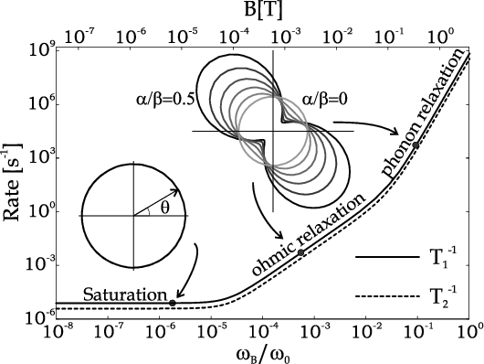
In section IV we present our results for the spin relaxation and decoherence rates in semiconducting quantum dots. We find that at low temperatures and low magnetic fields, T, Ohmic fluctuations originating from the electrodes dominate over the phonon effects in their infuence on the spin relaxation San-Jose et al. 2006. This is simply due to the fact that the spectrum of excitations of a metallic electrode is much denser than that of phonons at low energies. At still lower magnetic fields and temperatures, however, the dominant mechanism leading to relaxation is the accumulation of random geometric phases. This leads to a saturation of the decay rates at . Both features are included in the data shown in Fig. 1 and compared to previous predictions. Further results including the temperature dependence under typical experimental conditions are presented in section IV.
Finally, in Sec. V, we study an electron in an array of quantum dots and show that in the presence of SO interaction arbitrary spin rotations can be reached by a series of coherent electron tunneling processes in a multi-dot geometry. We discuss the possibility to use such multi-dot systems for geometric electron spin manipulations.
II Geometrical spin evolution in a semiclassical picture
II.1 Geometric phases and spin rotations
Geometrical phases, introduced in the pioneering work of Berry Berry 1984, describe how a quantum system in a non-degenerate state evolves when adiabatically driven around a closed loop in a control parameter space. Apart from a dynamical phase, depending on the energy and elapsed time, the state acquires a contribution, called the Berry phase, that only depends on the geometry of the loop in parameter space. An important extension of the Berry phase covers the case when the initial state belongs to a degenerate subspace Wilczek and Zee 1984. Then the geometric phase is replaced by a non-Abelian unitary transformation of the initial state within the degenerate subspace, and again, this unitary transformation depends only on the geometry of the loop.
This non-Abelian generalization of the Berry phase is of direct relevance for an electron confined in a quantum dot: Time reversal symmetry in the absence of a magnetic field implies that the spectrum of a quantum dot is a collection of time-reversed Kramers doublets even in the presence of spin-orbit interaction. In the absence of SO coupling these states correspond to pure spin states. In the general case the doublets persist, and we call them pseudospin states.
The adiabatic variation of the position (and possibly shape) of the potential confining the electron is described by a time-dependent Hamiltonian . Adiabaticity ensures that an electron which at time is in the ground state doublet remains within the corresponding subspace of instantaneous ground states of . The adiabatic time evolution thus appears as a non-Abelian SU(2) transformation within the ground state doublet Wilczek and Zee 1984. In the presence of spin-orbit coupling the unitary transformation results in a geometric spin rotation, which only depends on the trajectory of the electron in real space.
To illustrate the geometric spin rotation in more detail we consider a 2DEG, assumed to be grown along the direction. An electron in the 2DEG experiences a spin-orbit coupling which takes the form (, axis along the direction)
| (1) |
Here denotes the momentum of the electron in the plane of the 2DEG and is the spin operator. The Rashba () and linear Dresselhaus () couplings can be lumped into the spin-orbit tensor
| (2) |
An implicit summation over the coordinates is assumed, i.e. . The tensor sets the scale for the spin-orbit length , that defines the typical length scale of spin textures. In typical GaAs/AlGaAs semiconductor heterostructures we have .Amasha et al.
We further assume that by lateral structuring of the 2DEG a parabolic quantum dot, , is created with energy scale related to the orbital size . Typical dot sizes are in the range . Hence is usually small, of the order of . The electron is assumed to be strongly confined in the ground state of the potential. By applying electric fields (modifying the confining potential) we move the dot and the electron along a trajectory .
In the considered limit, , the degenerate doublet of states of the confined electron simply differ in the spin orientation. Eq. (1) then implies that the confined spin experiences an effective magnetic field, , with . For a strongly confining potential we have . Therefore the induced spin-evolution is described by Coish et al. 2006
| (3) | |||||
with and denoting time- and path-ordering operators, respectively. The tag ‘ad’ refers to the constraint of adiabatically slow paths, , which guarantees that the evolution affects the electron spin but does not induce transitions to excited dot states. Clearly, depends only on the geometry of a given path itself, not on the time dependence of . As we shall show in Sec. III.1, this result can be generalized to larger parabolic dots for which spin texture effects are important. The main difference in that case is that is replaced by a renormalized tensor .
In order to visualize the spin rotation described by Eq. (3) it is instructive to use the connection between SU(2) and SO(3) rotations. The change of the orientation of a sphere rolling on a plane along a path is characterized by a rotation operator
| (4) | |||||
where the components of denote the standard SO(3) generators. Comparing (3) and (4) and choosing the radius of the sphere to be we note that a spin rotation associated with a path maps onto a rotation of the sphere rolling along a trajectory (see Fig. 2). If only Rashba coupling is present then the paths and have the same shape. In general, if also Dresselhaus coupling is present, then and have different shapes, but the qualitative analogy persists.

In a 2DEG, with both Rashba and Dresselhaus couplings present, the change of the spin orientation induced by moving the confined electron along a straight line depends on the direction of trajectory relative to a crystal axis. The distance to perform a spin-flip is strongly anisotropic for , being enhanced in the direction. This property is illustrated in Fig. 2(b).
II.2 Spin manipulation and spin relaxation
To illustrate how the geometric phase evolution given by Eq. (3) can be used to manipulate the spin state we consider a quantum dot orbiting times around a closed circular path, , with period . The spin-orbit length is assumed much larger than the loop size, . For simplicity we assume pure Dresselhaus coupling. The resulting spin precession is then described by , where the evolution operator of a complete loop is
To second order in it reduces to
| (8) |
where denotes the area enclosed by a loop. As will be shown in Sec. III.1, Eq. (8) is valid for small closed loops of arbitrary shape. The full time evolution after circles can be approximated as
| (9) |
where is the area swept by repetitions of the loop. Obviously the motion in small closed loops corresponds to an effective static magnetic field, pointing along the -direction.
Eq. (9) also holds if the trajectory is a stochastic variable, typically induced by a fluctuating electric field, . In this case the area in Eq. (9) is a random variable whose dispersion increases linearly in time, . Assuming that is Gaussian distributed, we conclude that off-diagonal elements of the spin density matrix decay as
| (10) |
Thus the accumulation of - random - geometric phases leads to dephasing, even in the absence of external magnetic fields. The coefficient introduced above depends on the amplitude and frequency of typical electromagnetic fluctuations, and its proper computation requires a fully quantum-mechanical treatment of the electromagnetic field San-Jose et al. 2006, reviewed in Section III.2. At this point we note that the area itself is proportional to the square of the electric field, , with the typical frequency of electromagnetic fluctuations, and the characteristic time for making a closed loop is . Hence, the geometrical relaxation rate is proportional to . E.g., for Ohmic fluctuations we have and consequently the corresponding relaxation rate scales as . Note that this geometric dephasing is of fourth order in and, therefore, requires fourth order perturbation theory in the electromagnetic field.
II.3 Spin relaxation in a magnetic field
So far we assumed that no external magnetic field is applied. Now we study the relaxation and dephasing of a spin in an in-plane magnetic field in the presence of a classical stochastic field, , characterized by the power spectrum
| (11) |
The external field induces a precession of the spin around its direction with Larmor frequency , while the fluctuating field leads to relaxation and dephasing with rates and , given to leading order by the standard expressions Bloch 1957; Leggett et al. 1987; Weiss 1999
| (12) | |||||
| (13) |
Here and are the spectral densities of the components of perpendicular and parallel to , and the superscript , introduced to distinguish from later extensions, refers to second order. In case of isotropic random motion of the dot and purely Rashba (or purely Dresselhaus) spin-orbit coupling we have . Typically if the electron remains localized in space, since only unbounded paths can produce a static . Therefore the last term of Eq. (13) vanishes in this case and we obtain in leading order Golovach et al. 2004 .
We can also estimate the relaxation rate induced by the Berry phase mechanism, which is of higher order than expressions Eqs. (12) and (13): The effective magnetic field generated by the Berry phase term is proportional to , and is perpendicular to the in-plane magnetic field. The relaxation rate of the spin to fourth order in the coupling to the stochastic field is proportional to the Fourier component of the autocorrelation function of this effective field at frequency ,
| (14) |
where and refer to the spectral functions of the components and , parallel and perpendicular to the in-plane magnetic field.
Strictly speaking, Eqs. (12-14) hold only in the limit . In the opposite case, , also referred to as the Zeno regime, the relaxation times and lose their meaning, and other dissipative rates need to be considered. Although and vanish fast in the limit , saturates and scales to a finite value. This is because the Berry phase relaxation can also be induced by independent fluctuations of frequency , that have a ’beating’ (frequency mismatch) at frequency , which is in resonance with the Larmor spin precession. As a result, for sufficiently small but finite one always ends up in the Zeno regime, dominated by the Berry phase term, Eq. (14).
III Beyond the semiclassical approach
In this section we provide a fully quantum-mechanical treatment of a confined electron’s spin. We do this in two steps: First, we describe quantum-mechanically the spin and orbital state of the confined electron in a classical time-dependent electric field. Then, we generalize this within a path integral formalism to include quantum-mechanical fluctuations of the electric field.
III.1 Adiabatic approach in a classical electric field
III.1.1 Motion in a parabolic dot
To be specific, let us first consider an electron in a parabolic confining potential with energy scale corresponding to a typical orbital size . For the moment we will assume that the magnetic field is zero. In the presence of an applied or fluctuating classical in-plane electric field the Hamiltonian takes the form
| (15) | |||||
with being a time-dependent constant of no relevance, and . Thus the effect of the homogeneous electric field is to move the center of the potential along a trajectory, . We assume that . Then the Hamiltonians for times are related by the displacement operator ,
| (16) |
The center of the potential, , is our external control parameter in the language of geometric phases. Eq. (16) allows us to construct the instantaneous eigenstates of from the eigenstates for , as . The states come in Kramers doublets with and denoting their pseudospin orientation. We now introduce the ’adiabatic states’ or ’center of motion states’ as
| (17) |
Here the state satisfies the time-dependent Schrödinger equation with the Hamiltonian , while the adiabatic states move together with the dot and satisfy the equation of motion
| (18) |
Using the explicit form of the operator we thus find, apart from a trivial overall phase generated by , that the evolution of is described by the effective Hamiltonian
| (19) |
and the corresponding evolution operator,
| (20) |
Clearly, from the above equations it follows that if at time the electron occupies the ground state Kramers doublet, i.e., , and the external perturbation changes sufficiently slowly in time, , then the second term in Eq. (19) cannot generate transitions to the excited states of , and stays within the ground state doublet, . Under these conditions the effective Hamiltonian can be approximated as
| (21) |
where is the projector to the ground doublet of , and we took the energy of the ground state to be . The corresponding adiabatic evolution operator within the center of motion ground state subspace then reads
| (22) |
Although not obvious, the spin-orbit coupling plays an essential role in Eqs. (21) and (22). As shown in Appendix A we have,
| (23) |
where we introduced the non-trivial spin-dressing tensor 11 1 In general one would expect to be matrix, but due to reflection symmetry of the Hamiltonian, there is no coupling between the in-plane and components of the spin and pseudospin, and hence only the in-plane block of is relevant. , that relates the matrix elements of the spin operator to the pseudospin operator . Thus an adiabatic motion induces a pseudospin rotation within the ground state multiplet. Note that the formulas above are not perturbative in the spin-orbit coupling, and they hold for parabolic dots of any size compared to the spin-orbit length as long as the external field fluctuations are adiabatic. Thus the effects of strong spin-orbit coupling can be fully taken into account by replacing by the dressed spin-orbit tensor , so that the adiabatic evolution operator becomes
| (24) |
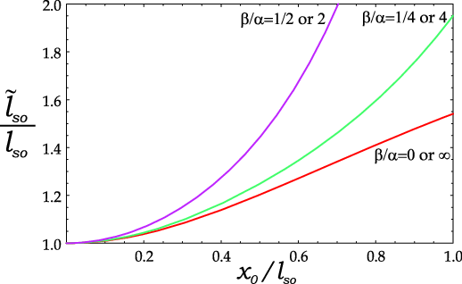
with being again the path ordering operator. From Eq. (24) it is obvious that the renormalization of the g-factor is also reflected in the renormalization of the relevant spin-orbit length scales, . This renormalized has been shown in Fig. 3 as a function of the ratio . In small quantum dots, , one has , and therefore , in agreement with the assumptions of Sec. II.
III.1.2 Connection with perturbation theory
The preceding discussion relied on the specific model of a parabolic quantum dot, which enabled us to construct the instantaneous eigenstates of the Hamiltonian for arbitrarily large but slowly changing displacements, . An alternative approach to construct that is valid for an arbitrary shape of the confining potential is to use perturbation theory in the driving term of Eq. (15) to determine the instantaneous eigenstates of San-Jose et al. 2006. This perturbative approach has the disadvantage of breaking down for displacements comparable to the typical dot size . However, in a conventional setup of single quantum dots defined by lithographic gates, one is usually constrained to small displacements such that the perturbative approach remains useful.
In the absence of external magnetic fields the perturbation does not connect states within the same doublet due to time reversal symmetry. One can then approximate the lowest energy instantaneous eigenstate as
| (25) |
where for brevity we have denoted by the energy of doublet at time , and . Then the effective adiabatic Hamiltonian, describing the evolution of the center of motion wave function within the ground state multiplet, reads
where the operators project to the ’th doublet state of the unperturbed Hamiltonian . Furthermore, in this equation we dropped full differential terms involving that give no contribution for closed paths, and we denoted by the components of the electron position operator. The above expression coincides with the limit of the results obtained previously using a more general perturbative approach in Ref. San-Jose et al. 2006.22 2 We denoted this term by in Ref. San-Jose et al. 2006 Treating the general case, , within this approach requires some care since the appropriate perturbation theory is quasi-degenerate San-Jose et al. 2006; San-Jose et al. 2007.
While it is not obvious, the above perturbation expansion approach and the displacement operator results presented in the previous subsection are equivalent. Due to the slightly different choice of the transformation the two approaches yield different adiabatic evolution operators, however, both Hamiltonians describe the same physical pseudospin precession, and physical observables are independent of this choice of basis. To illustrate this, let us compare the two matrices after a path that starts and ends at the origin. For a closed path , the perturbative approach yields a pseudospin transformation that can be expressed as
| (26) |
As we show in Appendix A, for the particular case of a parabolic dot sum rules imply that simplifies to
| (27) |
On the other hand, the exact displacement operator approach of the previous subsection yields
| (28) |
For a closed path with a small enclosed area we can approximate this expression by expanding to second order in the exponent and re-exponentiating as
| (29) | |||||
| (30) |
Eqs. (26), (30) and Eq. (27) imply that both approaches yield identical results. Furthermore, in the case of a parabolic dot we can show using the alternative form for , Eq. (24), that for small closed paths the evolution operator of the unshifted states, is approximately given as
| (31) |
where is displacement area spanned by the path. This generalizes the semiclassical result of the previous section to the case of arbitrary spin-obit coupling.
III.2 Treating the electromagnetic field quantum-mechanically
In the first part of this section we assumed that the time-dependent electric field acting on the electron is classical. However, if the typical frequency of the field reaches the temperature then the electric field must be treated quantum-mechanically. To treat the quantum fluctuations of the electromagnetic field, we shall employ a hybrid formalism, where we describe the fluctuations of the electromagnetic field within the path integral approach, while the quantum dot shall be treated within an operator formalism. Here we only summarize the results, the details of the calculation are presented in Appendix B.
For simplicity, we consider an electron spin in a parabolic quantum dot and dipolar electric fields as in subsection III.1.1. Then the adiabatic evolution operator that describes the evolution of the dot state for given initial and final states of the electromagnetic environment within the ground doublet is given by
| (32) | |||
| (33) | |||
| (34) |
Here the functional integral is performed over all possible fluctuations of the bath, , each of them corresponding to a different path between times and . We also allowed for the presence of an in-plane magnetic field , small compared to the level spacing of the dot, . The adiabatic displacement operators in Eq. (32) transform the wave function of the dot to the center of motion basis, , where the evolution is described by Eq. (20), projected by the projector to the lowest lying two eigenstates of , in the absence of the magnetic field.
Thus the pseudospin evolution under a quantum electric field is the coherent sum of classical evolutions over all possible field fluctuations weighted by the action of the decoupled bath, . We remark here that is not the non-interacting bath action, , but contains a correction due to the back reaction of the dot (see Appendix B). For a Gaussian we thus mapped the evolution of the spin to the well-studied spin-boson model, where, however, external bosonic fluctuations are coupled both to the x and y components of the spin. Castro Neto et al. 2003; Novais et al. 2005
To describe dephasing and spin relaxation at the fully quantum-mechanical level we generalized the formulas above to the evolution of the reduced density matrix for the pseudospin in the center of motion basis,
| (35) |
where stands for a trace over the bath degrees of freedom, is the density matrix of the complete dot-bath system, and . Note that now is an operator instead of a c-number, and that acts both on the bath and on the quantum dot. Then spin relaxation and decay corresponds to the diagonal and off-diagonal components of , respectively. The initial state of the system should not affect the dynamics at long times Hakim and Ambegaokar 1985, so we will assume the dot-plus-bath system to start at in a well defined ground doublet and the bath in thermal equilibrium, . This choice is technically convenient and physically describes a definite initial state with slightly entangled bath and dot states. Then the evolution of can be described as
| (36) |
where now runs along the usual double branch time contour running from to and then back to , as depicted in Fig. 7 in Appendix C, and is time ordering along this contour. Here denotes the average over the electromagnetic field fluctuations along the Keldysh contour,
where and denote the electric field along the upper and lower branches of the contour and satisfy the boundary condition, .
Unfortunately, one cannot integrate out the electric field exactly. However, one can use the systematic diagrammatic approach of Ref. [Schoeller and Schön 1994] to do perturbation theory in and obtain the relaxation rates within a Markovian approximation. Makhlin et al. 2002 The results of this calculation are presented in the following Section.
IV Results for relaxation and dephasing
We are now ready to summarize the results that are obtained by the formalism developed in the previous section. Some technical details of the calculation are presented in Appendix C. We remark here the present systematic approach confirms what had been derived within the perturbative formalism developed in Ref. San-Jose et al. 2006. Unlike in said work, where numerical results for were computed in a limited set of cases, the results for and presented in this section are fully analytical, which therefore allows for an explicit analysis of the decay rate dependence with all relevant physical parameters, such as magnetic field orientation, spin-orbit coupling or quantum dot size.
We have computed the spin relaxation () and dephasing () rates of confined electrons subject to an in-plane (renormalized) magnetic field at an angle with respect to direction . To fourth order in the spin-orbit coupling we obtain
| (37) | |||||
| (38) |
Here , is the quantum dot size (assumed parabolic) and the functions and are defined as
with the spectral function of the dimensionless electric field, , defined in Appendix C. Functions relate to the used in Appendix C by . Note that both and vanish for , while remains finite. Therefore, this latter part of the fourth order contribution can be identified as the Berry phase contribution. Indeed, this expression is identical to the one we obtained previously in Ref. [San-Jose et al. 2006]. Note also that this term is isotropic and does not depend on the direction of the magnetic field, while all other second and fourth order contributions do so for . In the formulas above we assumed that the spectral functions of the components of the dimensionless electric field are isotropic, .
The spectral function gives the density of electromagnetic excitations that contribute to dephasing, and it depends on the specific source of electromagnetic fluctuations. Important sources of electric field fluctuations are piezoelectric phonons Khaetskii and Nazarov 2000 and at low magnetic fields Ohmic charge fluctuationsSan-Jose et al. 2006,
For the case of piezoelectric phonons an estimate of the spectral function of the induced dimensionless electric field is outlined in Appendix D. For GaAs/GaAlAs heterostructures we obtain , with . At higher magnetic fields (frequencies) these fluctuations give the dominant contribution to spin relaxation/dephasing.
At low magnetic fields (low frequencies), on the other hand, Ohmic charge fluctuations of the electric environment of the 2DEG near the dot are expected to dominate. For these, the spectral function is for Fermi liquid leads, with , being the impedance of the leads. It is rather difficult to compute the exact value of , since it depends on the precise geometry of the leads and one must also take into account how the equilibrium electric field fluctuations inside the 2DEG extend to the quantum dot, and to what extent those fluctuations can be screened. It is not unreasonable, however, for typical sheet resistances of to assume .
In our calculations we have neglected the feedback correction that changes the action . In the case of the phonon bath, the effect of this term is to make phonons somewhat softer close to the dot. However, this polaron-type effect should be small, since the mass of the electron is negligible compared to the atomic masses. The feedback correction might be more important for the Ohmic bath, but will only affect , not the Ohmic character of the bath.


Implicit in the derivation of Eqs. (37) and (38) is the assumption that the effect of the thermal bath leads to an adiabatic evolution of the spin in the quantum dot. In physical terms one can anticipate that this implies a condition for the bath temperature , so that the dot is not heated above the ground doublet by the bath fluctuations. More precisely, the classical adiabatic condition given in Sec. II.1, translates in this context into the relation . For typical parameters in the case of the ohmic bath this means indeed . For the piezoelectric phonon bath this implies , where is the bath temperature in Kelvin. Non-adiabatic corrections are beyond the scope of this work, although they could in principle be taken into account in the calculation of Appendix C.
The first (second order) term in Eq. (37) is proportional to at small Larmor frequencies. Concentrating on this term one concludes that the relaxation and dephasing rates vanish for Khaetskii and Nazarov 2000; Stano and Fabian 2006; Semenov and Kim. The second and third terms in Eq. (38), which are of fourth order in the spin-orbit couplings, involve a convolution of the spectral function at frequencies up to the temperature scale, and does not vanish at low fields and non-zero temperature. Therefore the relaxation rates saturate both for the phonon and the Ohmic baths as the field is lowered. We remark that the sum of the terms and resemble the formula, Eq. (14), anticipated in Sec. II.3, although the full quantum treatment given here is necessary to identify precisely the functions and in Eq. (14) and to arrive at consistent quantitative predictions.
In Fig. 4, we plot the relaxation rates induced by the Ohmic and phonon baths separately for two different sets of parameters. For small magnetic fields (but still above the Zeno regime) the relaxation rates reach a clear saturation regime, with values
| (39) | |||
where the numerical constants equal equal , and .
As the field is increased, the second order terms begin to dominate. At low enough temperatures Ohmic fluctuations become dominant first, since their weight grows faster at low fields than the phonon contribution. Thus below a certain temperature there is a window of magnetic fields in which the relaxation rates have a scaling form characteristic of an Ohmic bath,
At still larger values of the magnetic field the phonon fluctuations dominate the second order relaxation channel, and the rates assume a ’phononic’ scaling form,
These cross-overs are shown in Fig. 5 for both relaxation and dephasing rates. The different regimes are summarized in a ’phase diagram’, which we show for typical parameters in Fig. 6.
As noticed in Ref. Golovach et al. 2004, up to second order in the coupling (i.e. at high fields). This relation is violated by the fourth order terms due to the contribution in (38), but is again restored in the saturation regime, where the fourth order term not considered in Ref. Golovach et al. 2004 vanishes.
For second order terms that dominate the high field behavior have a strong dependence on : . Their contribution to the relaxation rate is enhanced for fields along [110], especially as approaches for a fixed (see Fig. 5). This is easy to understand by looking back at Fig. 2(b). The relaxation of the spin occurs due to dot displacements along directions that flip the spin, which for spins along the [110] direction () are displacements along [110] itself (recall the geometric interpretation as a rolling sphere). As we see from Fig. 2(b) such angles are the most effective to induce spin flips, so the relaxation and also decoherence rates increase for fields in those directions, especially for the highly anisotropic case . In contrast, as is obvious from Eq. (39) and Fig. 2(b), at low fields the rates are dominated by the geometric term that is independent of .
V Electric spin manipulation
In the previous sections we investigated how in the presence of spin-orbit interaction stochastic and fluctuating fields lead to decay and decoherence of electron spin states. In the present section we discuss how one can use this effect in a constructive way to control spins purely by electric fields. For this purpose one should displace the quantum dot which confines the electron. Unfortunately, under realistic conditions such displacements are rather small compared to . Nevertheless, a series of small closed paths can be designed to take the spin of the confined electron to an arbitrary final state. In this way one can realize an all-electrical universal single qubit gate, under the realistic condition that the scattering mean free path in the 2DEG (typically in the range) is much larger than the confinement lengthscale . Another option that we shall discuss in this section is to move an electron in a system of quantum dots controlled by gate voltages, and in this way manipulate its spin state.
Closed trajectories of the electron (in a confining dot) covering an area induce a spin precession approximately given by Eq. (31) around the axis, in the same way as if a constant magnetic field was applied in this direction. In order to induce arbitrary spin rotations, e.g. spin flips, we have to rely on more complicated paths. An example is a path composed of sum of closed loops of period and area and another, much slower, closed trajectory of period and area , i.e., a spirograph-type of path. One can demonstrate that by properly choosing the relation between frequencies and trajectories, after a long enough driving time the spin can be driven to an arbitrary final state. The optimal relation for a spin-flip operation is . Due to the adiabaticity requirement, however, the minimal spin-flip time using this method for realistic values of the maximum displacement becomes several orders of magnitude slower than current flip times achieved using ESR techniques Koppens et al. 2006. The operation time can be reduced by using heterostructures with larger spin-orbit couplings, such as InAs. It can also be reduced substantially if we substitute the effect of the fast path component by an equivalent external static magnetic field along the direction, in which case the technique resembles closely previously proposed ac electric-field generalizations of ESR techniques Duckheim and Loss 2006.
One can, however, also use different methods to transport a confined electron over distances comparable or greater than the spin-orbit length . Surface acoustic waves, e.g., have been used to move electrons over large distances and to rotate their spins Stotz et al. 2005. Another possibility involves a ring of several tunnel-coupled quantum dots spanning distances comparable to . The electron can then be adiabatically shifted around the ring by appropriate time-dependent gate voltages. As we show below, such a manipulation can result in a large spin rotation, and thus provide a completely different principle than ESR, since no resonant AC fields would be involved. For this reason it could be expected to enable relatively fast coherent spin manipulation, since, unlike ESR, a single pumping cycle could be enough to induce a complete spin flip.
The discussion of pumping around the ring of dots can be reduced to sequential pumping processes between adjacent dots. We shall therefore analyze the precession of the (pseudo)spin of an electron that is transferred between two dots of sizes and separation smaller than . We further assume that a strong barrier between the dots remains present at all times during the pumping process, and use a tight-binding approximation. In this spirit, we write the Hamiltonian of the double dot structure as
| (40) |
where denotes the confining potential of the two dots at positions and , and the potential is generated by the external gate voltages, assumed to be small. Within the tight binding approximation the low energy states of the double dot system are a linear combination of the ground state wavefunctions of the isolated dots described by the Hamiltonians
| (41) |
In the considered limit the SO coupling can be treated perturbatively, and the Hamiltonians can be partially diagonalized by the unitary transformation , with
Here and is the angular momentum with respect to the center of the dot. Let us now assume that the confining potentials are cylindrically symmetrical and also that the ground states of are in the sector. Then the ground state of the individual dots can be approximated, to order , as
| (42) |
in terms of the spinor and the orbital eigenstate of with the spin-orbit coupling set to zero. This allows us to evaluate the matrix for the truncated and express it as
| (43) |
with the submatrices given by . Apart from a trivial overall shift of the energy, the diagonal blocks can be written as
| (44) |
being the potential difference between the dots. However, spin-orbit coupling generates a spin texture for the dot eigenstates, and results in a non-trivial spin-mixing in the in the hopping submatrix, :
| (45) | |||||
| (46) |
where is the vector connecting the two dots. In the second line we used the expression (42) and exploited the fact that the integrals pick up their major contributions from the regions and . We thus obtain,
where is essentially the tunneling distance in units of the spin-orbit length and the spin-independent hopping integral above. The angle characterizes the hopping direction and is defined through the relation . The SU(2) operator is the same we obtained in Eq. (24) for the geometric spin precession along a straight path connecting the two dots.
Diagonalizing this Hamiltonian matrix we obtain the instantaneous eigenstates with and corresponding to the ground and first excited doublets of the double dot structure. They are pairwise degenerate at any time and have energies and , with the splitting between the two doublets,
| (50) |
We shall now study the electron spin’s evolution within the adiabatic approximation: we look for a solution of the Schrödinger equation in the form . Then the wave function amplitudes satisfy the equation of motion
| (51) | |||||
If the time-derivatives in this expression are small compared to the splitting the evolution of the confined electron is adiabatic and is confined to the lowest doublet of the double dot. Remarkably, it is possible to write down such instantaneous ground states, satisfying the conditions ,
| (52) | |||||
| (53) | |||||
With this choice of basis the time evolution is trivial in the adiabatic approximation, and apart from an overall phase the wave function is simply given by
| (54) |
Now imagine making an adiabatic sweep, with the potential difference going from at time to at time . The above states have been chosen so that they satisfy the initial condition at , and describe an electron localized in the left potential well with (pseudo)spins . According to the above expressions, at time , i.e. after the adiabatic potential sweep , the electron will be found fully localized in the right dot and in the following spin superposition
| (55) |
independently of . In other words, the spin undergoes a spin precession identical to that obtained for upon adiabatically displacing a parabolic confining potential a distance along a straight line, Eq. (24). Although in our discussion we assumed a cylindrical symmetry for the dots, a slightly modified version of this discussion carries over to the case of non-cylindrical potentials with a spin rotation of comparable size. In general, however, the spin rotation is not given by the simple expression (55).
The most straightforward way to build a tunable gate on this concept would be to add a magnetic flux across a ring of quantum dots as a tuning parameter. Alternatively one could use backgates on top of the heterostructure to tune the Rashba spin-orbit coupling strengths around the ring.
VI Conclusion
In this article we have shown that for single electrons confined in quantum dots in a 2DEG, which is shifted adiabatically along a path by applied or fluctuating electric fields, the spin-orbit interaction induces pseudospin precession within the ground state Kramer’s doublet. In the absence of external magnetic fields, the precession depends solely on the geometrical shape of the trajectory of the confined electron. This accumulated non-Abelian phase has marked consequences for the spin relaxation and decoherence due to electric field fluctuations. In particular it leads to a saturation of the relaxation rates at vanishing magnetic fields. We have analyzed how the properties and power spectrum of the electromagnetic fluctuations influences the spin relaxation rates. We characterized two different spin decay regimes, dominated by Ohmic or phonon-induced electric fluctuations, respectively, and their crossovers as a function of external magnetic field and temperature.
The geometric spin precession analyzed in this paper can also be used to manipulate the spin state purely by controlling electric fields. We have shown that arbitrary rotations can be achieved by moving the dot along suitable trajectories. To speed-up the process we suggest moving the electron by adiabatic tunneling between quantum dots in multi-dot devices.
Acknowledgements: We would like to thank W. A. Coish and D. Loss for inspiring discussions. This research has been supported by Hungarian grants OTKA Nos. NF061726, T046267, T046303. G.Z acknowledges the hospitality of the CAS, Oslo.
Appendix A Various matrix element relations for a parabolic potential
For the parabolic quantum dot Hamiltonian, Eq. (15), we have the following identity:
where is the electron position operator, and is the dot displacement, assumed to be zero at . Here is the eigenvalue of the instantaneous eigenstates, , which are related to the eigenstates of as . Similarly, the expectation value of reads
Combining both equations above we obtain
| (56) |
We made use of the fact that commutes both with and , and therefore and . Specifically, for the ground state doublet (or lowest lying two states) this equation reduces to the useful identity
| (57) |
where are usual Pauli matrices. All spin-dressing corrections are contained in the matrix , whose definition trivially follows from Eq. (57), and simplifies to Eq. (23) in the absence of magnetic field.
Appendix B Pseudospin evolution under quantum fields
In this appendix we generalize Eq. (24) obtained for an electron confined in a parabolic well to the case where electromagnetic fields are produced by a quantum bath, which we shall treat within the path integral formalism. We assume that the bath is governed by Hamiltonian , while the coupling between the bath and quantum dot is of dipolar form, . We further allow for a Zeeman field coupled to the dot,
| (58) |
To combine the path integral approach with the adiabatic approximation, we write the evolution operator of the coupled system as
| (59) |
and insert the identity operator
| (60) |
after each time slice. Here denotes the identity operator acting on the dot, and . Note that the acts both on the bath and on the quantum dot, and now is an operator instead of a c-number. In Eq. (60) we also made use of the fact that the electric field operator is Hermitian and one can construct a complete basis from its eigenstates. However, being a local operator, every such state is infinitely degenerate. We keep track of this internal degeneracy by the label .
The matrix elements connecting two consecutive identity insertions labeled by and , take the following
| (61) | |||
where the operator , acts now only on the dots subspace, just as in Sec. III.1.1.
Using , the second term can be expanded in and written as
After re-exponentiating this expression Eq. (61) simply becomes
| (62) |
where is effective bath Hamiltonian.
The rest of the derivation follows the standard construction of the path integral except that we also insert the identity operator (60) before and after the evolution operator . The evolution operator of the dot for fixed initial and final bath states and , takes the form
| (63) | |||
Here the functional integral is performed over all possible paths of bath states with definite compatible with the endpoints and , each of them corresponding to a different path of the displacement . Bath paths begin at and end at . The weight comes from the prefactor in (62), and involves the effective bath Hamiltonian . Its dependence on the extra quantum numbers is already integrated out. Finally, the operator inside the integral is acting only on the quantum dot, and has exactly the same form as Eq. (20) for a classical field.
Since electric field fluctuations are assumed to be slow and the magnetic field is small, the time ordered operator in Eq. (63) can be approximated by its adiabatic form. Projecting this operator to the ground state subspace of with , we have
| (64) |
After using identity (57) of the previous appendix this expression reduces to Eq. (32), given in the main text.
Appendix C Diagrammatic calculation of relaxation and decoherence rates
We can generalize the calculation of the previous appendix to compute the evolution of the center of mass reduced density matrix, defined as in Eq. (35),
| (65) |
We use the Schrödinger representation and insert the identity operator (60) for both the forward and backward propagation in the expression of the full density matrix . This leads to the following expression [recall definitions (33) and (34)]
where denotes the initial center of mass density matrix. The integration should be performed on the complex contour, , and denotes the time ordering along this contour.
We define an operator describing the propagation of between different times
| (66) |
In perturbation theory in the geometric coupling between the dot and the electric field we can construct a corresponding Dyson equation for the propagator ,
where
is the bare propagator. In the following, we shall assume that the initial center of mass density matrix factorizes as , where represents some density matrix of a non-interacting Gaussian heat bath.
Then the ’self-energy’ has an expansion in Feynman diagrams along the contour, with vertices at branch corresponding to terms , in the expansion (see Fig. 7). Differentiating with respect to and defining the Liouvillian as , one arrives at the master equation
This equation can be simplified under the Markovian approximationMakhlin et al. 2002, where we assume that relaxation and dephasing are slow and therefore replace in the second integrand to yield
with the Bloch-Redfield tensor defined as
Relaxation and dephasing times and are then trivially related to this tensor asMakhlin et al. 2002
| (67) | |||||
| (68) |
A ’rotating wave approximation’ is implicit in these relations that requires in our particular case, see Sec. II.3.

Let us now perform a calculation of and to fourth order in the coupling between the dot and the electromagnetic field, for a small quantum dot with negligible spin dressing ( and ). Assuming an in-plane magnetic field at an angle with respect to the direction [100] we have
The eigenvalues of are , where . In the particular doublet basis which diagonalizes we can write , and equals
with the indices ordered as ). This basis is rotated with respect to the original one by an operator , so that our vertex in branch , reads in this basis
where and the relevant transverse and parallel dimensionless couplings, and , are defined by
| (69) |
For compactness, we shall use the vector notation in the rest of this appendix. The corresponding vertex matrices and at time at branch that enter the expansion of (are denoted by blue dots in Fig. 7, and read
In this notation we have the following relation for the -th order contribution to Bloch-Redfield tensor in the dot-bath coupling
| (80) | |||||
Here , i.e. a time-ordered integral over the internal times is implicit, and the bracket denotes averaging over the bath fields , i.e. pairwise contractions for a non-interacting (Gaussian) bath. Only connected contributions must be taken into account in the averaging, and all odd contributions average to zero. The and diagrams are represented in Fig. 7. The case has two types of distinct contractions that correspond to contracting the vertices at and with each-other and with internal vertices, respectively (represented in two separate rows in Fig. 7). Each contraction gives a non-interacting bath Green’s function defined in the Heisenberg picture as
Here once more refer to the time branch, and the time evolution of the operators in the first line is governed by . For simplicity, we assume an isotropic bath so that .
In the literature, one commonly denotes in the off-diagonal components as and . The spectral function is related to these as , while the Keldysh propagator is given by . Since is a real bosonic field, in equilibrium we have
| (81) |
where is the Bose distribution, and is the spectral function of the rescaled bath field . This spectral function can be easily related to the spectral function of the dimensionless electric field, as . Both spectral functions are odd in .

The second order results for and take the known form Leggett et al. 1987; Weiss 1999
| (82) | |||||
| (83) |
The fourth order contributions to are obtained by summing all corresponding diagrams. They are rather involved, but have the general structure
| (84) |
The kernel contains delta functions of . In Fig. 8 we plot the lines along which these delta functions pick up their contribution for relaxation and dephasing. We can distinguish two types of lines. The diagonal lines in the 2nd and 4th quadrants lead to convergent integrals, since goes exponentially to zero at large values of . Diagonal lines with positive slope and also horizontal and vertical lines across the origin cancel out exactly in . The remaining horizontal and vertical lines exhibit ultraviolet divergencies, and give therefore cutoff dependent prefactors that multiply and . These terms can thus be reabsorbed in the second order result by simply renormalizing the couplings . The final result can then be expressed in terms of these renormalized constants as
| (85) | |||||
| (86) |
where the functions are given by the following convolutions of
| (87) | |||||
The Green’s functions and can be expressed in terms of the spectral function of the dimensionless electric field , introduced below Eq. (81)
| (88) |
Inserting these last equations into the expression (87) one arrives at the results in Eqs. (37) and (38). The spectral function for electromagnetic fluctuations generated by piezoelectric phonons is computed in the next appendix.
Appendix D Phonon bath properties
Let us consider the fluctuating electric field induced by the phonons in the sample holding the quantum dot. The electric field acting on the confined electron is the gradient of the potential generated by these phonons, . It has two contributions, one from a longitudinal mode and another from two transverse modes
| (89) |
with indicating the mode. The coupling to the longitudinal is given by Cheng et al. 2004
while the coupling to the transverse mode is
Here , is volume, is the depth of the quantum well where the 2-dimensional electron gas is confined. The function , being the Heaviside function, qualitatively accounts for the truncation of the phonon spectrum out of the 2DEG plane.Golovach et al. 2004 The physical origin of this cut-off is that phonons having a wave-vector component larger than along the direction cannot couple efficiently to the confined electron, since their wave function oscillates too quickly. The density , the sound velocities and , and the piezoelectric constant in the expressions above are material-dependent parameters, which depend on the particular heterostructure used to define the quantum dot: for a typical GaAs/AlGaAs heterostructures , , , and .
The noise power of the normalized electric field can be expressed as
It can be checked that and are indeed independent in this model.
Using , and we see that the only dependence on the orientation of the wave vector vector appears through . We can therefore introduce spherical coordinates in the continuum limit and integrate with respect to the angular variables. For the longitudinal phonons this yields
| (90) | |||||
where the function above comes from the truncation of the phonon spectrum, and is given by
| (91) |
The two transverse modes give a similar contribution
| (92) | |||||
with
| (93) |
The cut-off functions and play a role similar to , but have algebraic tails: for large , while . The phonon spectrum is defined as usual by .
Taking the Fourier transform of the correlation functions above, we can identify the spectral function ,
| (94) | |||||
| (95) | |||||
where and . For frequencies smaller than the cutoffs we obtain for GaAs/AlGaAs quantum wells. Note that in this calculation we neglected the lateral size of the dot. That provides an additional cut-off for the in-plane phonon momentum for larger values of the frequency .
References
- Elzerman et al. (2004) J. Elzerman, R. Hanson, L. van Beveren, B. Witkamp, L. Vandersypen, and L. Kouwenhoven, Nature 430, 431 (2004).
- Petta et al. (2005) J. Petta, A. Johnson, J. Taylor, E. Laird, A. Yacoby, M. Lukin, C. Marcus, M. Hanson, and A. Gossard, Science 309, 2180 (2005).
- Koppens et al. (2006) F. H. L. Koppens, C. Buizert, K. J. Tielrooij, I. T. Vink, K. C. Nowack, T. Meunier, L. P. Kouwenhoven, and L. M. K. Vandersypen, Nature 442, 766 (2006).
- Loss and DiVincenzo (1998) D. Loss and D. P. DiVincenzo, Phys. Rev. A 57, 120 (1998).
- Kato et al. (2005) Y. K. Kato, R. C. Myers, A. C. Gossard, and D. D. Awschalom, App. Phys. Lett. 86, 162107 (2005).
- Hankiewicz et al. (2006) E. M. Hankiewicz, G. Vignale, and M. E. Flatte, Phys. Rev. Lett. 97, 266601 (2006).
- Engel et al. (2005) H. A. Engel, B. I. Halperin, and E. I. Rashba, Phys. Rev. Lett. 95, 166605 (2005).
- Awschalom and Flatte (2007) D. D. Awschalom and M. E. Flatte, Nature Physics 3, 153 (2007).
- Duckheim and Loss (2006) M. Duckheim and D. Loss, Nature Physics 2, 195 (2006).
- Bulaev and Loss (2007) D. V. Bulaev and D. Loss, Phys. Rev. Lett. 98, 097202 (2007).
- Golovach et al. (2006) V. N. Golovach, M. Borhani, and D. Loss, Phys. Rev. B 74, 165319 (2006).
- Stano and Fabian (a) P. Stano and J. Fabian, cond-mat/0611228.
- Tang et al. (2006) J. M. Tang, J. Levy, and M. E. Flatte, Phys. Rev. Lett. 97, 106803 (2006).
- Stotz et al. (2005) J. A. H. Stotz, R. Hey, P. V. Santos, and K. H. Ploog, Nature Materials 4, 585 (2005).
- Kato et al. (2004) Y. Kato, R. C. Myers, A. C. Gossard, and D. D. Awschalom, Nature 427, 50 (2004).
- Abrahams (1957) E. Abrahams, Phys. Rev. 107, 491 (1957).
- Dyakonov and Perel (1972) M. I. Dyakonov and V. I. Perel, Soviet Physics Solid State,Ussr 13, 3023 (1972).
- Khaetskii and Nazarov (2000) A. V. Khaetskii and Y. V. Nazarov, Phys. Rev. B 61, 12639 (2000).
- Khaetskii and Nazarov (2001) A. V. Khaetskii and Y. V. Nazarov, Phys. Rev. B 64, 125316 (2001).
- Woods et al. (2002) L. M. Woods, T. L. Reinecke, and Y. Lyanda-Geller, Phys. Rev. B 66, 161318(R) (2002).
- Golovach et al. (2004) V. N. Golovach, A. Khaetskii, and D. Loss, Phys. Rev. Lett. 93, 016601 (2004).
- Sherman and Lockwood (2005) E. Y. Sherman and D. J. Lockwood, Phys. Rev. B 72, 125340 (2005).
- San-Jose et al. (2006) P. San-Jose, G. Zarand, A. Shnirman, and G. Schön, Phys. Rev. Lett. 97, 076803 (2006).
- Stano and Fabian (2006) P. Stano and J. Fabian, Phys. Rev. B 74, 045320 (2006).
- (25) Y. G. Semenov and K. W. Kim, cond-mat/0612333.
- Serebrennikov (2004) Y. A. Serebrennikov, Phys. Rev. Lett. 93, 266601 (2004).
- Stano and Fabian (b) P. Stano and J. Fabian, cond-mat/0512713.
- Berry (1984) M. V. Berry, Proc. R. Soc. London A 392, 45 (1984).
- Wilczek and Zee (1984) F. Wilczek and A. Zee, Phys. Rev. Lett. 52, 2111 (1984).
- (30) S. Amasha, K. MacLean, I. Radu, D. M. Zumbühl, M. A. Kastner, M. P. Hanson, and A. C. Gossard, cond-mat/0607110.
- Coish et al. (2006) W. A. Coish, V. N. Golovach, J. C. Egues, and D. Loss, Physica Status Solidi B-Basic Solid State Physics 243, 3658 (2006).
- Bloch (1957) F. Bloch, Phys. Rev. 105, 1206 (1957).
- Leggett et al. (1987) A. J. Leggett et al., Rev. Mod. Phys. 59, 1 (1987).
- Weiss (1999) U. Weiss, Quantum dissipative systems (World Scientific, Singapore, 1999), 2nd ed.
- San-Jose et al. (2007) P. San-Jose, G. Schön, A. Shnirman, and G. Zarand, in Proceedings of DECONS06 (Dresden, May 2006) (accepted in Physica E, doi:10.1016/j.physe.2007.05.027, 2007), eprint arXiv:0704.2974v1 [cond-mat.mes-hall].
- Castro Neto et al. (2003) A. H. Castro Neto, E. Novais, L. Borda, G. Zarand, and I. Affleck, Phys. Rev. Lett. 91, 096401 (2003).
- Novais et al. (2005) E. Novais, A. H. Castro Neto, L. Borda, I. Affleck, and G. Zarand, Phys. Rev. B 72, 014417 (2005).
- Hakim and Ambegaokar (1985) V. Hakim and V. Ambegaokar, Phys. Rev. A 32, 423 (1985).
- Schoeller and Schön (1994) H. Schoeller and G. Schön, Phys. Rev. B 50, 18436 (1994).
- Makhlin et al. (2002) Y. Makhlin, G. Schön, and A. Shnirman, in NATO-ASI Proceedings, edited by R. Fazio, V. F. Gantmakher, and Y. Imry (Kluwer, Erice (Italy), 2002), pp. 197 – 224, cond-mat/0309049.
- Averkiev et al. (2006) N. S. Averkiev, L. E. Golub, A. S. Gurevich, V. P. Evtikhiev, V. P. Kochereshko, A. V. Platonov, A. S. Shkolnik, and Y. P. Efimov, Phys. Rev. B 74, 033305 (2006).
- Cheng et al. (2004) J. L. Cheng, M. W. Wu, and C. Lu, Physical Review B (Condensed Matter and Materials Physics) 69, 115318 (2004).