Inhomogeneous exclusion processes with extended objects:
The effect of defect locations
Abstract
We study the effects of local inhomogeneities, i.e., slow sites of hopping rate , in a totally asymmetric simple exclusion process (TASEP) for particles of size (in units of the lattice spacing). We compare the simulation results of and and notice that the existence of local defects has qualitatively similar effects on the steady state. We focus on the stationary current as well as the density profiles. If there is only a single slow site in the system, we observe a significant dependence of the current on the location of the slow site for both and cases. When two slow sites are introduced, more intriguing phenomena emerge, e.g., dramatic decreases in the current when the two are close together. In addition, we study the asymptotic behavior when . We also explore the associated density profiles and compare our findings to an earlier study using a simple mean-field theory. We then outline the biological significance of these effects.
pacs
05.70.Ln, 87.15.Aa,05.40.-a 87.15.Aa, 05.40.-aI Introduction
A better understanding of non-equilibrium steady states in interacting complex systems forms a critical goal of much current research in statistical physics. In this pursuit, the totally asymmetric simple exclusion process (TASEP) Krug; Derrida92; DEHP; S1993; Derrida; Schutz has played a paradigmatic role. It provides a nontrivial, yet exactly solvable, example of phase transitions far from equilibrium, taking place even in one-dimensional (1D) lattices. At the same time, it also serves as the starting point for the modeling of many physical (driven diffusive) processes, such as translation in protein synthesis MG; LBSZia; TomChou, inhomogeneous growth processes (e.g. Kardar-Parisi-Zhang growth) KPZ; WolfTang and vehicular traffic Chowdhury; Popkov.
In its simplest version, the TASEP involves a single species of particles hopping to nearest-neighbor sites, in one direction only, along a homogeneous 1D lattice. Provided the destination site is empty, the rate for the particle hop is fixed at (typically chosen as unity without loss of generality). With periodic boundary conditions, the steady-state distribution is trivial Spitzer but the full dynamics is quite complex Gwa; Kim; BM. With open boundary conditions, particles are injected with rate (in units of ) at one end and drained with rate at the other end. The competition of injection, transport and drainage induces a nontrivial phase diagram in the - plane Krug; Derrida92; DEHP; S1993; Derrida; Schutz, reflecting a highly nontrivial steady state. Three phases are present: a maximum-current phase for , and a low- (high-) density phase for , (, ). Not surprisingly, there are also rich dynamical aspects deGier; AZS.
To model protein synthesis, each site on the lattice represents a codon on the messenger RNA (mRNA), and the particles represent the ribosomes. Injection, hopping, and drainage are associated respectively with initiation, elongation, and termination in biological terms. The quantity of interest, namely, the (steady-state) protein production rate, is identical to the (stationary) particle current. Clearly, the simple TASEP falls short of the biological system in several significant aspects. One is that an individual ribosome “covers” several codons MG; Heinrich; Kang, as opposed to a particle occupying only a single site. Another is that, in all naturally occurring mRNAs, the codons carry genetic information and therefore necessarily form an inhomogeneous sequence. Thus, the elongation rate of a ribosome is unlikely to be uniform; instead, the hopping rate, , of a particle becomes a function of the site . For example, it is well known that translation slows down at specific codons (see, e.g. Solomovici; Stenstrom; TomChou; Chou9; Chou10), with potentially significant consequences for protein production rates. Indeed, the steady-state current may depend sensitively on not only the frequency of each codon’s occurrence, but also the order of their appearance in the sequence. Both of these issues – extended objects and inhomogeneous rates – have been addressed recently in separate contexts which we summarize briefly in the following.
The results associated with inhomogeneous (quenched random) rates fall into two broad categories, in the sense that the randomness can be associated with the particles EnaudDerrida16; EnaudDerrida23; EnaudDerrida24 or with the sites. Randomness of the former type is more relevant for vehicular traffic where it accounts for a variety of driver preferences. In contrast, the disorder in the protein case is clearly site-dependent, leading to spatially non-uniform hopping rates . Restricting ourselves to this class, we can consider the effect of having a whole distribution, or very specific configurations, of . Starting from given distributions, two groups TripathyBarma; Harris studied the resulting disorder-average in periodic systems. To mention just one significant effect, the current-density diagram develops a plateau: limited by the smallest rate in the system, the current becomes independent of density over a range of densities. Harris and Stinchcombe Harris also extended this work to open systems. While these studies may be of some interest to mixtures of many different mRNAs, our primary interest here is to understand how the production rate of a specific protein is associated with a specific genetic sequence. As a first step towards a solution, we adopt the approach of several other studies Kolo; HadN; LBS; TomChou, by focusing on the effects of a few localized inhomogeneities, i.e., hopping rates which are uniform except at a handful of sites note1. As a synthesis of these studies, we will explore in some detail the consequences of having extended objects and locating one or two slow sites at a variety of positions on the lattice. In this manner, by introducing more and more sites with a range of rates, we hope to understand inhomogeneities in a systematic way, setting the stage for further investigations of the translation process.
A full comprehension of the effects of slow sites on the particle current may have potentially significant applications in biotechnology. While there are 64 distinct codons, proteins are chains composed of just 20 amino acids. So, many different mRNAs (codon sequences) can code for the same particular protein. Moreover, the amino acid is incorporated into the growing chain by an important intermediary, the so-called transfer RNA (tRNA), which carries the complementary anticodon. It turns out that the mapping between codons and tRNAs is also not precisely 1-1. For example, in E. coli, the genetic code actually involves 61 sense codons and about 46 tRNAs with associated anticodons Neidhardt. Meanwhile, for a given mRNA sequence, the protein production rate is often modeled in terms of (generally accepted) charged-tRNA (aminoacyl-tRNA, or aa-tRNA) concentrations Solomovici, so that different sequences can result in different production rates for the same protein. By elucidating how the spatial distribution of defects, especially of bottlenecks, affects translation rates, we can pinpoint those clusters of codons which are likely to have the most significant effect on the production rate of the associated protein. Exploiting the degeneracy in the mapping from mRNA sequence to protein, we can provide guidance as to how a few selected, local modifications of the mRNA can optimize the production rate of a given protein.
Our paper is organized as follows. In Section II, we define the model and provide a more detailed description of previous work, concerning exclusion processes with extended objects or spatially inhomogeneous rates. A brief discussion of a previous mean-field analysis is also included. In Section III, we present our Monte Carlo results. We focus especially on the implications of having extended objects by varying the particle size. We first consider the interaction between one slow site and the system boundary, and, motivated by the resulting findings, turn to the interactions between two slow sites. This provides new insights for genes containing clusters of slow codons, which occur frequently in, e.g., E. coli, Drosophila, yeast and primates Chou11; Chou14; TomChou. In Section IV, a complete investigation of systems with inhomogeneities is presented using a mean-field approach. Section V contains our conclusions and a summary of open questions.
II Model specifications and known results
The TASEP is defined on a 1D lattice of sites. We introduce an index to label the sites. Each site (codon) is either occupied by a single particle (ribosome) of length (in units of sites) or empty. A microscopic configuration of the system can be uniquely characterized in terms of a set of occupation variables, , taking the value 1(0) if site is occupied (empty). Of course, the extended nature of the particle induces strong correlations in , in the sense that a single ribosome always covers consecutive sites. Yet, at any given time, only one of the covered codons is being “read” (i.e., the codon is “covered by the aminoacyl site”, or A site, of the ribosome) and translated into an amino acid. Here, we refer to the associated location on the ribosome as the “reader” (of the genetic code). For our purposes, it is not essential which one of the sites is labeled as the reader, and so we follow the convention in LBSZia and choose the first (leftmost) site. Hence, the statement “a ribosome (or particle) is located at site ” implies that the reader is located at site and the subsequent
| (1) |
sites are also occupied. Naturally, the position of the reader determines the elongation rate, i.e., , since the ribosome must wait for the arrival of the aa-tRNA with the -specific anticodon before it can move to the next site. Clearly, the reader locations can also be used to label a microscopic configuration, i.e., we can define the reader occupation number at site as . The sets and are uniquely related to each other. Moreover, due to the extended size of a particle, strict constraints are built in (e.g., implies and ). As a consequence, neither set can be arbitrary and serious correlations arise as soon as note2.
In our simulations, we adopt a random sequential updating scheme and keep a list of locations of readers. In addition, the site is always occupied by a “virtual reader,” which accounts for particles entering the system (initiation). At the beginning of each Monte Carlo step (MCS), we first find the number of particles in the system and label it . Then, we randomly select an entry from this list of readers. If the chosen reader is virtual (i.e., ), a new particle enters the lattice with probability , provided all the first sites are empty. If the chosen reader is real, say, at site , the associated particle is then moved to site with probability , provided site is empty. With this notation, we can also write the initiation and termination probabilities ( and ) as and , respectively. To be complete, the sites beyond the lattice are by definition empty, so that once a particle reaches , it will not experience steric hindrance (see Fig. 1 for a sketch of this process). These processes have been termed “complete entry” and “incremental exit” Lakatos. Other entry and exit rules can be considered, but are believed to be inconsequential provided . Each MCS consists of such attempts, giving an even chance, on average, for each particle (ribosome) in the system to elongate or terminate, as well as for an initiation event to occur.


Starting with an empty lattice, we typically discard MCS to ensure that the system has reached the steady state. Unless otherwise noted, good statistics result if we average over least measurements, separated by MCS in order to avoid temporal correlations. Such steady state averages will be denoted by . To reduce the number of parameters in the model, we study systems with , except at one or two sites. The system sizes () range from to , with most data taken from .
To characterize the state of the system, we monitor several observables. The most obvious is , a quantity we will refer to as the ribosome (or reader, or particle) density. Of course, is just the average number of particles in the system (i.e., ribosomes on the mRNA). Thus, the overall particle density is bounded above by . Another interesting variable , labeled as the “coverage density”, is the probability that site is covered by a particle (regardless of the location of the reader). Needless to say, the profile for the vacancies is given by the local hole density, . The overall coverage density, , may reach unity and provides a good indication of how packed the system is. The two profiles are related by
| (2) |
with the understanding for .
A quantity of great importance to a biological system is the steady-state level of a given protein. If we assume that the degradation rates are (approximately) constant, i.e., independent of protein concentration, then these levels are directly related to the protein production rates. In our model, such a rate is just the average particle current , defined as the average number of particles exiting the system per unit time. In the steady state, it is also the current measured across any section of the lattice. For simplicity and to ensure the best statistics, we count the total number of particles which enter the lattice over the entire measurement period (at least MCS in most cases).
In this study, we focus on two simple types of inhomogeneities: one or two “slow” sites (Fig. 1). Their locations specify the only inhomogeneities in the rates.
One slow site, at position . We denote by (). This corresponds to a bottleneck in the lattice. We are especially interested in the dependence of the current, denoted by , on the parameters and .
Two slow sites, at positions and with separation and rates We find that, when , the current is controlled mainly by the smaller of the two, with little dependence on , in agreement with a simple mean-field theory to be discussed in Section IV. Therefore, most of our attention will be devoted to the case with . Moreover, we choose to limit our study to both sites being far from the boundaries. Then, the current is insensitive to their average position , and we can investigate . Note that these are precisely the systems studied in TomChou, except that we consider particles with a range of sizes: and . While there are qualitative similarities, we will discuss the quantitative differences due to , as well as interesting phenomena associated with the density profiles.
Let us now provide the context of our work by briefly reviewing some related earlier studies. The homogeneous case () with is exactly soluble Derrida92; DEHP; S1993; Derrida; Schutz, and displays three phases in the - phase diagram. For , no exact solutions existnoExact. Analytic approximations using various mean-field approaches MG; Heinrich; Lakatos; LBSZia; SS predict the presence of the same phases, though the phase boundaries depend on (Fig. 2) through the combination LBSZia
| (3) |
Monte Carlo studies Lakatos; LBSZia largely confirm these conclusions.

The three phases carry different currents and display distinct density profiles Derrida92; DEHP; S1993; Derrida; Schutz; Lakatos; LBSZia; LBS. Apart from “tails” near the boundaries, the (coverage) density profiles approach uniform bulk values in the thermodynamic limit, i.e., , for . For and , the system is in a low-density phase (L), characterized by and . A high-density phase (H) prevails for and , with bulk density and current . For , the system is in a maximum-current phase (M), where and . On the line (dashed line in Fig. 2), the system consists of two macroscopic regions, characterized by a low (high) density region near the entry (exit) point. The two regions are joined by a shock front that performs a random walk. This is often referred to as the “shock phase” (S). Table 1 summarizes the relation for TASEP with extended objects.
| phase | current | bulk density |
|---|---|---|
| L | / (1 + ) | /(1 + ) |
| H | / (1 + ) | |
| M |
There is good agreement between simulations (with ) and analytic results for these bulk quantities Lakatos; LBSZia. The details of the profile for , especially near the lattice boundaries, are less well understood. While periodic structures (of period ) can be expected, mean-field theories MG; Heinrich; Lakatos were successful in capturing only a limited part of the phenomena observed. We will return to these considerations in Section IV. Beyond homogeneous systems, several studies introduced one or more “impurities” into TASEP with periodic boundary condition. A single “slow” site induces a shock in the density profile with some interesting statistics Janowsky; JandL; HadN13; HadN14; HadN15. Subsequently, generalizations to systems with a finite fraction of slow sites, randomly located, were also investigated TripathyBarma. For the richer case of the open boundary TASEP Kolo; HadN; LBS; TomChou; DSZ, Kolomeisky focused on point particles (), with a single impurity at the center of the lattice Kolo, so as to mimic a defect situated deep in an infinitely long system. The consequences of the defect having both faster () and slower () rates were explored. By matching two ordinary TASEPs across the defect, the properties of such systems in the - plane can be well described Kolo; DSZ. While a fast site has no effect on the phase diagram, a slow site leads to a shift of the M-H and M-L phase boundaries to -dependent, smaller values of and . The density profiles are quite sensitive to the existence of a defect site Kolo; TomChou. Kolomeisky’s approach was generalized to the case in LBS, with similar levels of success. Below, we will provide further details of this work, on which we base much of the analysis of our problem. Ha and den Nijs also studied the open boundary TASEP with a single defect at the center HadN. Focusing on the multicritical point , they were mainly interested in the so-called “queueing transition” and its critical properties. Detailed results of density profiles, such as power law behavior and critical exponents, were obtained in the region . Here, denotes the critical value of below which the bulk density in front of the slow site deviates from the density behind the blockage. By contrast, our focus here is essentially that of TomChou; DSZ, namely, how does the number and the locations or spacings of the slow sites affect the current through the system? In the single slow site case, TomChou investigated mainly the overall current as a function of , while DSZ analyzed the current as a function of (the distance between the defect and the entry point). For the case of two defects, both studies find that the spacing between them plays a significant role for the current. A finite-segment mean-field theory in TomChou provides excellent agreement with data. In particular, clustered defects reduce the current much more effectively than well separated ones. In this sense, we can regard these investigations as exploring the “interactions” between the slow site(s) and/or the boundaries. Since both studies are restricted to point particles (), our intent is to explore the effects of having extended objects (with ). Though we expect qualitatively similar behavior, as pointed out in TomChou, we also find noteworthy quantitative differences. Finally, we should mention that larger numbers of defects do not lead to significantly different effects TomChou, so that we limit ourselves to one or two slow sites here.
III Monte Carlo results
In this section, we present our Monte Carlo results. For convenience, we use a consistent color coding scheme (online only) for the various particle sizes, as specified in Table 2.
| size | online color |
|---|---|
| 1 | black |
| 2 | red |
| 4 | brown |
| 6 | green |
| 12 | blue |
The data here consist of the overall currents and the density profiles of both coverage and ribosomes. Our focus will be how these quantities depend on , (for the case with a single defect), and (for the case with two defects). Although the profiles are difficult to extract experimentally, the reader profiles will be of interest in subsequent studies involving real gene sequences, since they provide information on how frequently a particular tRNA is bound to the mRNA. By contrast, the currents are easily measurable and our results here may generate more immediate interest.
III.1 One slow site
We begin by placing one slow site on the lattice as in Fig. 1(a). Fig. 3 shows several coverage density profiles for a typical choice of parameters: , , and with . As expected, we observe pile-ups of particles due to the blockage – a high (low) density region before (after) the bottleneck in all three cases. However, due to the lack of ordinary particle-hole symmetry in the cases, the average densities on either side of the slow site are not symmetric around . Instead, they are roughly related through the - relations in the H and L phases, summarized in Table 1. In detail, the profiles are quite different: The “tails”, i.e., the deviations from the bulk values, are quite noticeable in the vicinity of both the slow site and the edges of the system for the cases. The inset exposes more clearly that there are period structures in the profiles MG; Heinrich; Lakatos, especially just before the slow site.

A more dramatic difference between point particles and extended objects emerges when we plot the ribosome density , in Fig. 4, corresponding to the inset in Fig. 3. Similar to profiles in MG; Heinrich; Lakatos, we find distinct period structures before the slow site. While the reader “waits” to pass the blockage, the readers of the following particles tend to catch up and pause at sites , where . The “tails” are even more marked than those in Fig. 3. To emphasize the difference between the reader and coverage profiles ( and ), we show a case with in Fig. 5. Though both profiles contain the same information, we see that (lower plot) is far more sensitive than (upper plot) in showing the very long tails ( in this example) hidden in the collective behavior of the particles. At present, the crucial ingredients that control the characteristic decay length of the -envelopes have not yet been identified. Certainly, these very large length scales are completely absent from the systems deep within the H/L phases.


As for the current, Fig. 6 illustrates its dependence on , , and . Not surprisingly, the current is limited by the bottleneck and therefore varies monotonically with . It is also reduced if the particle size increases, an effect that can be traced mainly to the particle density being effectively lower by the factor . For point particles, the current is not very sensitive to the location of the slow site. The enhancement as approaches the boundary of the system – referred to as the “edge effect”DSZ – is quite small. For larger , the enhancement is much more pronounced, especially for smaller . Whatever the magnitude, in all cases the current increases monotonically as the slow site is located closer and closer to the entry point. For , particle-hole symmetry is manifest in the microscopic dynamics, so that the symmetry of under inversion, is obvious DSZ. For , the density profiles confirm the lack of this particle-hole symmetry very clearly. Correspondingly, there is a systematic asymmetry in the current: is satisfied only for . The origin of this behavior is not well understood.
The edge effect, and specifically its dependence on and , can be quantified by the ratio:
| (4) |
Fig. 7 shows that depends on in a nontrivial way. The maxima of occur at lower values of as increases, reminiscent of the behavior of the phase boundary between M and L/H. With appropriate scaling, the curves of can be collapsed for large ’s. From the biological perspective, the edge effect is not easily observable since the current enhancement is less than for the relevant .
Returning to Fig. 6, we note that significant deviations from the asymptotic value, , are found only for ’s within a small distance from the boundaries. At a casual glance, this range appears to depend on both and . On closer examination of, say, the most prominent case here: , we find that the decay of into fits an exponential quite well (Fig. 8), i.e., , with . Assuming this behavior persists in the other cases, we can study the dependence of this characteristic length and denote it by . We believe that the origin of this length scale can be traced to the presence of tails in the density profiles near the lattice boundaries: As the slow site approaches the entry point, these tails may seriously affect the injection process, and thus, the current as well. For the case, we observe that , where is the characteristic length associated with the boundary layer of the density profile in the ordinary TASEP. Specifically, with entry rate and exit rate , the system is in the H-phase and the profile decays exponentially into the bulk, as with Schutz:
| (5) |
Here, the left half of our system is such a TASEP, except that we have an effective : LBS. Using these arguments on the three ’s shown, we estimate decay lengths of about (), (), and () lattice constants. Though the data on the differences are small and noisy, simulation results are consistent with . However, for , there is no analytic result for the boundary layers of the density profiles. Moreover, the data suggest that they are quite complex (e.g., in Figs. 4 and 5). Thus, it is unclear how to quantify the picture for point particles to the general case of . At present, a complete understanding of both “boundary layers” – in the density profiles and in – remains elusive.

If we consider the edge effect as an “interaction” between the slow site and the lattice boundaries, the natural next step is to explore the interactions between two slow sites. In order to avoid edge effects, we place the two slow sites sufficiently far away from the boundaries and vary their separation.
III.2 Two slow sites
As mentioned in the previous section, the currents in the cases are essentially controlled by the slower of the two rates and so, may be regarded as systems with a single slow site. These profiles can be interesting, but we choose to restrict our attention here to a study of the case, in which the currents show a nontrivial dependence on , the distance between the two slow sites. With two bottlenecks, the system consists of three sections: before the first blockage, in between the two, and after the second defect. Of course, for small , the overall density in the first (last) section is expected to be high (low). In these cases, the effective entry and exit rates for the central section are also low, so that a wandering shock should be present. Hence, the average profile should be linear for (and essentially so for larger LBSZia) with a positive slope. This behavior is understandable, since the section between the two defects is comparable to an ordinary TASEP with small . These expectations are generally confirmed by simulations with and various ’s up to . Fig. 9 shows typical coverage profiles, for a relatively small rate of . The system appears to make a transition from this H/S/L phase to an M/M/M phase as increases. The center profiles become essentially flat, as illustrated in the inset (where and ). Details of this transition are being explored.

More interesting are the finer features of the profiles in the small cases. As in the single defect system, the profiles exhibit period structures near the slow sites. To resolve these more clearly, we plot the reader density profiles in Fig. 10. In all cases that involve extended particles (), the readers clearly pile up behind the slow sites. Apart from these “jams,” another feature emerges, namely, a sequence of depletion zones, each of which precedes one of the period peaks. For , the differences between the upper and the lower envelope are especially dramatic. More remarkably, when the blockages are separated by small ’s, two different, “overlapping tails” are created, as illustrated in the inset of Fig. 10, where , , and . Indeed, there are further interesting structures for , which will be presented elsewhere.

Compared to these remarkable characteristics in the profiles, the behavior of the currents seems lackluster. In Fig. 11, we plot four sets of currents note3, , associated with and . In all cases, we see that is considerably suppressed when is reduced. When the slow sites are very far apart, the current behaves as if there is only one slow site, consistent with expectations from mean-field theories. At the other extreme, when the two defect sites are nearest neighbors, the current reaches its minimum. Not surprisingly, period structures emerge as is varied, illustrated in the inset of Fig. 11(d), but become less prominent for . These plots also reveal that, unlike the dependence on above, there are serious deviations from the values when is decreased. To quantify this deviation, we define
| (6) |
and plot this quantity vs. in Fig. 12. In contrast to , we observe that exhibits a sizable dependence on , especially for small values of . In the limit of the current decreases by a factor of 2! In the following section, we will see that this factor can be understood via a mean-field approach.

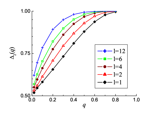
To summarize our simulation results, two bottlenecks near each other have a dramatic effect on the current. We may regard this phenomenon as an “interaction” between the two slow sites, inducing far more “resistance” when they are close than when they are well separated.
Two additional comments are in order. First, we return to one of the predictions of the mean-field theory, namely that a second slow site, spaced far apart from its partner, should have no further effect on the current. Our data indicate that the current for two slow sites, spaced far apart, is systematically lower than the current for a single slow site, but only by a very small amount (less than ). Second, we can again attempt to identify a length scale which controls how approaches , as increases. Since the central section of the system displays a shock, it is natural to ask whether the intrinsic width of the shock sets this length scale. According to Janowsky; JandL, this width covers only a few lattice spacings in the periodic TASEP with a single defect. Here, however, it appears that the shock is much broader. For example, the averaged profile of the shock for the case of with point particles is shown in Fig. 13, as well as a simple fit using a function note4 with width of about . Intriguingly, this length appears to be comparable to the one appearing in Fig. 11(a). More work is needed to fully explore these issues.

IV Mean-Field Theoretic Approaches
Mean-field theory is known to agree well with the exact results for a number of macroscopic quantities in the steady state of the TASEP (see, for example Schutz). For extended particles, no exact solution is available noExact so that mean-field (and more sophisticated cluster) approximations form the only route toward some understanding of the system’s behavior.However, there are many levels of “mean-field” approximations MG; LBSZia; Lakatos; LBS, corresponding to neglecting different types of correlations. For certain quantities (e.g., currents in large systems), predictions from the simplest level are very close to the simulation results. For others (e.g., some reader profiles), only the most sophisticated level performs adequately. In all cases, no level of mean-field theory can give a good fit to both the current and the profile. A thorough discussion of all of these schemes is quite involved and will be provided elsewhere promises. Here, we will restrict ourselves to the simplest method and compare its performance to the simulations.
All approaches start with the exact expressions for the current
| (7) | |||||
| (8) | |||||
| (9) | |||||
| (10) |
In the absence of the steady-state distribution, the most naive approximation is to replace by . Unfortunately, the constraints due to particles with are so severe that this approximation is entirely inadequate when . Even for the simple case of TASEP on a periodic ring, it leads to an erroneous expression for (except if ). Instead, the average (coverage) density at site is much larger than the (conditional) probability that it is actually covered given that the reader is at site . MacDonald and Gibbs (MG) proposed MG a much better approximation:
As discussed in Section II, the densities far from boundaries are uniform (e.g., ) and this fact provides a good description of the current-density relation
| (11) |
(for ). Exploiting this relation and regarding our model as two or three TASEPs joined by slow sites, the simplest level of mean-field theories can be built. Ours is similar to, but simpler than, the approach in LBS for the single defect case. The main difference lies in the matching condition, i.e., what approximate expression for the current across the slow site to use. After comparing the two approaches, we proceed to build the case for TASEP with two defects.
IV.1 One slow site
When a single slow site () is located at , the system can be treated as two sublattices: and , referred to as the left and right sublattices, respectively. Associated quantities will appear with subscripts and . The two sections are coupled through the slow site by having the same current in the steady state. Given this constraint, there are only two viable scenarios for the sublattices, out of the 33 logically possible ones: H/L and M/M.
First, let us consider the H/L case which was one studied extensively in LBS. The current for each sublattice can be written as:
| (12) |
where and are the effective exit and entry rates, to be determined later. By definition, the entire system reaches steady state when , which yields . Of course, these are intimately related to the (bulk) densities through and , so that
Another way to regard this relation is that both densities lead to the same current, which we denote by (a value to be determined, and equal to ). So, the high and low densities can be written as and , respectively, being the two roots to Eqn. (11). They will play a crucial role when we impose the matching condition, thereby fixing all quantities as a function of .
The exact equation for “matching” is
| (13) |
in which and lie in and , respectively. Now, the right can be expressed as, again exactly, , the probability for finding a ribosome at , conditioned on the presence of a hole at .
Since we have “broken” the system into two separate TASEPs, a naive approximation is to begin with
where the subscript stands for “naive mean field.” Regarding this as Eqn. (7) for the sublattice, we have . Now, is in the sublattice, and must be related to in a mean-field approach. The most naive assumption is that is the same as its average in the bulk, i.e., , which would be in this case. However, this turns out to underestimate seriously. Indeed, the “pile-up” near a blockage (e.g., in Fig. 5) shows that is significantly higher than its bulk value as well as the densities on the sites before. Thus, we propose that a better approximation would be to replace by , and we write
| (14) |
Using and , so that and
we arrive at . The premise behind this line of arguments is that the system is in H/L, so that both and should be less than . Therefore, this expression for the current should be valid only if it is less than the maximal value (). In other words, the domain of its validity is limited to . For higher , this approach predicts that the system will be in an M/M phase, with maximal current. Note that such a phase cannot occur with a slow defect in the case, where M/M can be accessed only with . In an earlier study LBS, the parameters chosen ( and ) also precluded the presence of this phase, although we believe (see below) that this phase cannot be present if the blockage is in the center () or deep in the bulk. We summarize this “naive mean field” by
| (15) |
An alternative approximation for eqn. (13) was proposed earlier LBS:
| (16) |
The last two factors can be recognized as and the MG approximation for the effective hole density MG. The first factor is a little more subtle LBS: Considering that the transit time for a single particle through the slow site (in the absence of steric hindrance) is , is defined as the average rate to move just one step in this process:
The end result for the current is the solution to the algebraic equation
Here, we give an explicit form (which displays the limit well)
| (17) |
where
Note that, for any , this approach predicts that the current is less than the maximal value of and so, the system is always in the H/L phase.

The results of both mean-field predictions for as a function of are shown in Fig. 14, along with two sets of data: and . As expected, was purpose-built for two infinite TASEP’s connected by a slow site and provides a better fit to the data with the blockage deep in the bulk ( in ). On the other hand, it is understandable that, e.g., for , must be very close to . Thus, we may expect that the system will have maximal current for . This behavior is confirmed by the data, as illustrated in the figure for . Since has the property that it saturates at for , it provides a better fit for . Of course, we recognize that, as mean-field theories, neither (14) nor (16) are the first step in a systematic expansion, so that they may better be thought of as “semi-phenomenological”.
More importantly, there is a more serious, inherent limitation in this level of mean-field theory. It cannot account for the full -dependence in , since it deals only with infinite systems. One possibility to incorporate finite-size effects (of the left sublattice) in this kind of theory is to exploit the MG expression MG
for sites near the boundaries. Using it in a recursion relation for finding both the density profile and the current, we will arrive at a -dependent expression, , which replaces in the first expression of Eqn. (12). However, the high density fixed point of this recursion relation is unstable and very careful numerical analysis will be necessary. Preliminary work on this approach is promising and will be reported elsewhere promises.
We end this subsection by noting that the effects of a single defect in TASEP have also been investigated in HadN. Unlike our focus here - the dependence of on the location of the slow site, they are concerned with a “multicritical system,” i.e., for the case. Putting the defect at the center of the lattice, they explored density profiles in detail, finding power law tails on both sides of the defect with -dependent exponents. By contrast, our choice of places us far from the multicritical point. We have no reason to expect similar power laws.
IV.2 Two slow sites
The most general TASEP with just two slow sites can be quite involved, since the parameter space is four-dimensional: . To carry out a manageable investigation, we let both sites be deep in the bulk, so that only the distance between them, , plays a significant role. Further, as pointed out above, the central section resembles an ordinary TASEP with and controlled by and , respectively. Therefore, it is the smaller (slower) of the two rates which limits that current, which in turn dictates the current through the whole system. Thus, we will focus only on the case. Our parameter space will then resemble the single slow site case.
Following the single defect case, the simplest levels of mean-field theory treat our system as three subsections with obvious labels: and . From our discussion, only two (out of the many logical possibilities) combinations of phases, H/S/L and M/M/M, are expected to be viable. In addition to Eqn. (12), we have
| (18) |
Since the defect rates are identical, we fully expect that, for such a mean-field theory, . Now, matching the currents of the subsections, we immediately arrive at and so, . From here, the “naive” mean-field approach for H/S/L proceeds identically to the above. The argument relies on the presence of a shock in the central section, so that there is a low (high) density region near site () and we can impose the same discontinuity in the densities across both defects, i.e., before and after. Thus, we again arrive at , given explicitly in Eqn. (15). The same argument can be applied to the next level of a mean-field approximation, which predicts , as in Eqn. (17). The major difference between the two approaches, as in the single slow site case, is the absence of the M/M/M phase in the latter. Meanwhile, their limitations are similar: The dependence in cannot be accommodated without serious modifications.
Nevertheless, the spirit of these approximations can be exploited to provide in the limit. Since the central section consists of just one site, there can be no shock. Instead, the remnant of the shock is reflected in the average density there. It is more convenient to regard the system as two infinite TASEP’s, with nontrivial matching across a “doubly - slow site.” Of course, we cannot expect to find any of the fascinating profile details (e.g., inset of Fig. 10), but we should be able to obtain the “coarser” information, such as the currents. The goal is to understand the behavior of (cf. Fig. 12) in, say, the first two non-vanishing orders in .
Now, for , we are naturally in the H/L phase and the crudest approximation should suffice for the lowest order in the current. So, we let the bulk densities be at their extremes (i.e., one and zero) and simply consider the time it takes for a particle to move through the blockage, from the moment its predecessor is “released.” The current is just the inverse of this quantity, i.e.,
| (19) |
where we have included terms for computing the next order. But, at this order, we should also take into account that, occasionally, the density before/after the blockage deviates from unity/zero by virtue of the right hand side of Eqn. (11) being non-zero. Thus, these densities are
and further suppress the current at the next-to-lowest order through the factor
| (20) |
Combining these factors, we arrive at
If we use exactly the same arguments for the limit current in the case of one slow site, we find, instead of (19),
| (21) |
and, instead of (20),
Finally, since is the same as the single-blockage current, we write
| (22) |
so that
It is remarkable how well this crude approximation agrees with the data in Fig. 12. There is no doubt that all curves extrapolate to the -independent value of at . As for the slope at the origin, we can obtain a good estimate from the lowest data points, using . The values obtained from simulations for and are and , respectively.
We are aware that the expansion (22) differs from the small limit of . Unfortunately, it is difficult to implement the same scheme for here, since we must start from the exact pair of equations:
| (23) |
Various attempts at approximating or led to poorer results. Alternatively, we could exploit the argument in SKL LBS and consider the average time to traverse both slow sites, . This gives us a new effective :
which can be inserted into Eqn. (16). The result is , the term of which differs from the data by about a factor of 2. Clearly, mean-field approaches are far from ideal for finding quantitative predictions of . On the other hand, either or provide tolerable results when the blockages are from from each other or the boundaries. Such variations in the quality of mean-field theories point to the importance of correlations. Considerable efforts appear to be necessary for a comprehensive, yet relatively simple, theory.
Let us end this section with another method which could possibly improve the theoretical predictions TCidea, especially for the first few values of . The idea is to find exact results, by solving the full master equation, for TASEPs (with extended objects) on very small lattices and then to match these to an infinite system (the sublattice). One expectation is that, as in the case, the finite-size current is larger than its counterpart for the infinite TASEP at the same . This approach may eventually provide the essential argument to understand the increase in as becomes smaller. Similarly, this idea can be applied to the case with two slow sites when is . Work is in progress to explore these avenues.
V Summary and conclusions
In this study, we consider an inhomogeneous TASEP with open boundaries and populated with particles of finite extent, . The hopping rates are uniform (set at unity) except for one or two sites (“defect bonds”), where the rates, , are different (faster or slower). We are interested in the effects of these local defects on the density profiles and the currents through the system. Simulations with various show that fast sites have no effect on the current, but induce discontinuities in the density profiles. In contrast, slow sites generate a significant reduction of the current as well as nontrivial structures in the profiles, e.g., long tails behind the blockage, with period . These findings are entirely consistent with similar studies in the past, most of which were restricted to Kolo; HadN. If the inhomogeneities are deep in the bulk and far from each other, the current depends only on and can be understood through simple mean-field considerations. Through the current-density relationship (for an infinite homogeneous TASEP), the overall densities in each of the defect-free sections can be also predicted, so that the various “phases” of these subsystems can be understood. The distinguishing feature in our study is how the location of the defects affects the behavior of the system. For the case of one slow site, the current is slightly but measurably enhanced when the defect approaches the boundary. On the other hand, a drastic reduction of the current is observed when two slow sites are brought closer to each other. It is tempting to interpret these effects as “interactions” between the defects and to seek a formulation that can describe them quantitatively.
At present, neither the enhancement nor the suppression of the currents can be understood in terms of simple mean-field theories. The essential limitation is that they are based on matching homogeneous TASEPs of infinite length. More sophisticated versions, relying on recursion relations for the particle density at each site, may be exploited to deal with the finite subsections and provide some promise for a better understanding of such effects. For very small subsections, such as , it may be possible to find exact solutions (even for ) that can be used to match the mean-field descriptions for the macroscopic subsection(s). Work is in progress to investigate these approaches systematically.
Beyond one or two blockages, we should study systems with multiple slow sites, as our eventual goal is to understand the properties of fully inhomogeneous TASEPs. In particular, though restricted to just one or two slow sites, our findings - that the relative locations of blockages are important - will have implications for translation. For example, they are directly applicable to “designer genes”, which consist of many repeats of the same codon, except at one or two locations. Using the abundance of associated aa-tRNAs as a control for the elongation rate across any particular codon, we can test our results directly on such genes. Thus, it will be interesting to see the physical manifestation of, e.g., enhancement and suppression of production rates of such artificial proteins, depending on the placement of the slow codon(s). Similarly, reproducing the intriguing ribosome density profiles will be revealing. More important than “designer genes,” we should consider the implications for real genes. Our results should provide, at the least, some simple qualitative insights. We can obviously maximize the production rate of a particular protein associated with a certain real gene by systematically replacing all slow codons with synonymous, faster ones. However, for most genes this operation will require a large number of replacements. Instead, with our findings in mind, we can achieve considerable increases in the production rates by making only a few substitutions, namely, by replacing the slowest codons, or a cluster of nearby slow codons. The ratio of current enhancement to the number of codon replacements may be used to quantify how “optimal” a certain set of substitutions is. This idea can be applied to finding optimal means to suppress prodcution rates as well. Simulation work with TASEPs associated with real genes is in progress and we hope to demonstrate that these concepts are viable.
Acknowledgements.
We have benefited from discussions with T. Chou, M. Evans, M. Ha, R. Kulkarni, P. Kulkarni, M. den Nijs, S.-C. Park, L.B. Shaw, and B. Winkel. We are especially grateful to M. Ha and M. den Nijs for providing their unpublished data. This work is supported in part by the NSF through DMR-0414122, DMR-0705152, and DGE-0504196. JJD also acknowledges the generous support from the Virginia Tech Graduate School.References
- (1) J. Krug, Phys. Rev. Lett. 67, 1882 (1991).
- (2) B. Derrida, E. Domany, and D. Mukamel, J. Stat. Phys. 69, 667 (1992).
- (3) B. Derrida, M.R. Evans, V. Hakim, and V. Pasquier, J. Phys. A: Math. Gen. 26, 1493 (1993).
- (4) G.M. Schütz and E. Domany, J. Stat. Phys. 72, 277 (1993).
- (5) B. Derrida, Phys. Rep. 301, 65 (1998).
- (6) G.M. Schütz, in Phase Transition and Critical Phenomena, Vol. 19, edited by C. Domb and J.L. Lebowitz (Academic Press, San Diego, 2000).
- (7) C. MacDonald, J. Gibbs, and A. Pipkin, Biopolymers, 6, 1 (1968); C. MacDonald and J. Gibbs, Biopolymers, 7, 707 (1969).
- (8) L.B. Shaw, R.K.P. Zia, and K.H. Lee, Phys. Rev. E 68, 021910 (2003). This article also contains a review of earlier work.
- (9) T. Chou and G. Lakatos, Phys. Rev. Lett. 93, 198101 (2004).
- (10) M. Kardar, G. Parisi, and Y.-C. Zhang, Phys. Rev. Lett. 56, 889 (1986).
- (11) D.E. Wolf, and L.-H. Tang, Phys. Rev. Lett. 65, 1591 (1990).
- (12) D. Chowdhury, L. Santen, and A. Schadschneider, Curr. Sci. 77, 411 (1999).
- (13) V. Popkov, L. Santen, A. Schadschneider, and G.M. Schütz, J. Phys. A: Math. Gen. 34, L45 (2001).
- (14) F. Spitzer, Adv. Math. 5, 246 (1970).
- (15) L. H. Gwa and H. Spohn, Phys. Rev. Lett. 68, 725 1992; and Phys. Rev. A 46, 844 (1992).
- (16) D. Kim, Phys. Rev.E 52, 3512 (1995).
- (17) S. Gupta, S. N. Majumdar, C. Godrèche, and M. Barma, Phys. Rev. E 76, 021112 (2007).
- (18) J. de Gier and F.H.L. Essler, Phys. Rev. Lett. 95, 240601 (2005).
- (19) D.A. Adams, R.K.P. Zia, and B. Schmittmann, Phys. Rev. Lett. 99, 020601 (2007).
- (20) R. Heinrich and T. Rapoport, J. Theor. Biol. 86, 279 (1980).
- (21) C. Kang and C. Cantor, J. Mol. Struct. 181, 241 (1985).
- (22) M. Robinson, R. Lilley, S. Little, J.S. Emtage, G. Yarranton, P. Stephens, A. Millican, M. Eaton, and G. Humphreys, Nucleic Acids Res. 12, 6663 (1984).
- (23) M.A. Sorensen, C.G. Kurland, and S. Pedersen, J. Mol. Biol. 207, 365 (1989).
- (24) J. Solomovici, T. Lesnik and C. Reiss, J. Theor. Biol, 185, 511 (1997).
- (25) C.M. Stenström, H. Jin, L.L. Major, W.P. Tate, and L.A. Isaksson, Gene 263, 273 (2001).
- (26) Z. Csahók and T. Vicsek, J. Phys. A: Math. Gen. 27, L591 (1994).
- (27) J. Krug, and P.A. Ferrari, J. Phys. A: Math. Gen. 29, L465 (1996).
- (28) J. Krug, Braz. J. Phys. 30, 97 (2000)
- (29) G. Tripathy and M. Barma, Phys. Rev. E 58, 1911 (1998).
- (30) R.J. Harris and R.B. Stinchcombe, Phys. Rev. E 70, 016108 (2004).
- (31) A.B. Kolomeisky, J. Phys. A: Math. Gen. 31, 1153 (1998).
- (32) M. Ha, J. Timonen, and M. den Nijs, Phys. Rev. E 68, 056122 (2003). For more details, see also M. Ha, PhD thesis, University of Washington, 2003.
- (33) L.B. Shaw, A.B. Kolomeisky and K.H. Lee, J. Phys. A: Math. Gen. 37, 2105 (2004).
- (34) In much of the physics literature, the term “bond” is used instead of “site”, since hopping is associated with a particle jump from site to site . However, in translation, a ribosome “at site ” can move to the next site only when the tRNA associated with site arrives. Therefore, it is natural to associate the jump rate with a site, and so we will use terms like “slow site” and “slow bond” interchangeably. With protein synthesis in mind, we also use the phrase “slow codon.”
- (35) F. Neidhardt and H. Umbarger, in Escherichia coli and Salmonella, 2nd ed. edited by F.C. Neidhardt (ASM Press, Washington D.C., 1996).
- (36) D.A. Phoenix and E. Korotkov, FEMS Microbiol. Lett. 155, 63 (1997).
- (37) S. Zhang, E. Goldman, and G. Zubay, J. Theor. Biol. 170, 339 (1994).
- (38) For TASEP on a ring, the total number of particles and holes are both conserved. If the hopping rates are uniform, it is possible to specify microscopic configurations in such a way that no such correlations are explicitly present, namely, the set of integers , where denotes the number of holes between the and particles. See e.g.TripathyBarma. However, this mapping is quite impractical for open TASEPs, since the number of particles (or holes) is a fluctuating quantity.
- (39) G. Lakatos and T. Chou, J. Phys. A: Math. Gen. 36, 2027 (2003).
- (40) Exact solutions for ASEP with extended objects have been obtained, but only for a closed system with periodic boundary conditions. See, e.g., F.C. Alcaraz and M.J. Lazo, Braz. J. Phys. 33, 533 (2003). Our main interest, motivated by translation in protein synthesis, is open systems, with non-trivial entry/exit rates (our /) and phases.
- (41) G. Schonherr and G. M. Schutz, J. Phys. A: Math. Gen. 37, 8215 (2004).
- (42) S.A. Janowsky and J.L. Lebowitz, Phys. Rev. A 45, 618 (1992).
- (43) G.M. Schütz, J. Stat. Phys. 71, 471 (1993).
- (44) B. Derrida, S.A. Janowsky, J.L. Lebowitz, and E.R. Speer, J. Stat. Phys. 73, 813 (1993).
- (45) S.A. Janowsky and J.L. Lebowitz, J. Stat. Phys. 77, 35 (1994).
- (46) Since the shock diffuses throughout the region between the slow sites, a relatively nontrivial method must be used to compile averages. Details will be published elsewhere promises
- (47) K. Mallick, J. Phys. A: Math. Gen. 29, 5375 (1996).
- (48) J.J. Dong, B. Schmittmann, and R.K.P. Zia, J. Stat. Phys. 128, 21 (2007).
- (49) J.J. Dong, B. Schmittmann, and R.K.P. Zia, to be published.
- (50) Note that the argument in now refer to the distance between the two slow sites.
- (51) We thank T. Chou for suggesting the approach used in TomChou.