Universality class of the pair contact process with diffusion
Abstract
The pair contact process with diffusion (PCPD) is studied with a standard Monte Carlo approach and with simulations at fixed densities. A standard analysis of the simulation results, based on the particle densities or on the pair densities, yields inconsistent estimates for the critical exponents. However, if a well-chosen linear combination of the particle and pair densities is used, leading corrections can be suppressed, and consistent estimates for the independent critical exponents , and are obtained. Since these estimates are also consistent with their values in directed percolation (DP), we conclude that PCPD falls in the same universality class as DP.
pacs
05.70.Ln, 05.50.+q, 64.60.HtI Introduction
In the fermionic one-dimensional pair contact process with diffusion (PCPD), the model studied here, point particles can diffuse on a line, and reactions can occur when two particles end up next to each other. The particles can then both be annihilated, or if there is a free site next to the pair, a new particle can be created. The reactions present in the PCPD model are:
with and .
As for other systems of this kind, the scaling relations which are expected to hold for the density and correlation length are
in which is the distance to the critical point. The critical exponents in these scaling relations define the universality class a system belongs tohinr00; marr96. Two firmly established universality classes so far for systems of this kind are the Directed Percolation (DP) and Parity Conserving (PC) classes.
Since the introduction of PCPD a decade ago howard97, or at least a model closely resembling it, it has attracted much attention. The main reason for this attention is that, while its symmetries and conservation laws are seemingly identical to directed percolation (DP), numerical estimates of its critical exponents seem to place it in a different universality class. It has been conjectured before by Grassberger grass82 and Janssen jans81 that critical points with a unique absorbing state and a single order parameter will fall into the DP universality class, making this a likely candidate for PCPD as well. However, the fact that the PCPD absorbing state is not unique makes this less certain, and it has been suggested by earlier studies that it might not be possible to describe PCPD with a single order parameter jans04; park05. Table 1 shows values reported for the critical exponents of PCPD from previous studies, as well as the accurately known values for these exponents in the DP universality class. So far, while it is obvious much research has been done on this subject, there is still a certain amount of disagreement in the results. Generally, the differences between the measured exponents and the values for directed percolation have been significant. It has been argued, however, that the discrepancy in between PCPD and DP is due to severe finite-size and finite-time effects bark03, and recent ultralong simulations hinr06 show a clear trend of towards its DP-value.
Other recent studies have looked at field theory approaches for PCPD jans04, and looked at a bosonic version of the model, where multiple particles can exist in one spot kock03; hinr06. Another study kwon07 has investigated the structure and behavior of clusters in PCPD, to clarify the slow approach of PCPD to its asymptotic scaling regime. Investigation of the crossover from PCPD to DP park06 has yielded evidence towards non-DP scaling.
At this point, it is still unclear what universality class PCPD does belong to. Most studies so far conclude that PCPD might belong to a new univerality class kock03; park06, or even that it might belong to several ones based on the value of the parameter odor00; dick02; park02; odor03. On the other hand, in a recent study by H. Hinrichsen hinr06, the critical exponent was shown to display a significant drift towards the DP value, providing evidence towards a single universality class. However, this tendency has not been clearly shown for the other two exponents so far.
A previous study (Ref. bark03) has provided numerical evidence that, at the critical point, the ratio between the pair and particle densities tends to a non-zero, finite value when the simulation time tends to infinity. Also the high-quality data of Ref. hinr06 confirms the convergence to a nonzero ratio. A visual inspection of the system shows big clusters, separated by increasingly large empty (or near-empty) regions. Since these clusters tend to have a finite density in particles as well as in pairs, the convergence of their ratio to a nonzero value is not unexpected.
Based on this convergence of the ratio of particles and pairs, we will show in this paper that PCPD has strong correction terms in its scaling relations when it has not yet reached the thermodynamical limit. These correction terms will distort any direct measurements of the exponent. The correction terms for these quantities, however, do not turn out to be exactly the same. We will show that if both the particle- and the pair-densities are combined in the analysis, these corrections can in some cases be suppressed, allowing a more accurate result for the exponents. The resulting estimates for the critical exponents of the PCPD model are consistent with the DP universality class.
| Study | Year | |||||
|---|---|---|---|---|---|---|
| Ódor odor00 | 2000 | 0.1 | 0.275(4) | 0.58(1) | - | - |
| 0.5 | 0.21(1) | 0.40(2) | - | - | ||
| 0.9 | 0.20(1) | 0.39(2) | - | - | ||
| Carlon, Henkel | 2001 | 0.1 | - | - | 1.87(3) | 0.50(3) |
| and Schollwöck carl01 | 0.5 | - | - | 1.70(3) | 0.48(3) | |
| 0.8 | - | - | 1.60(5) | 0.51(3) | ||
| Hinrichsen hinr01 | 2001 | 0.1 | 0.25 | 1.83(5) | 0.50(3) | |
| Park, Hinrichsen & Kim park01 | 2001 | * | 0.236(10) | 0.50(5) | 1.80(2) | - |
| Park & Kim park02 | 2002 | * | 0.241(5) | 0.496(22) | 1.80(10) | - |
| * | 0.242(5) | 0.519(24) | 1.78(5) | - | ||
| Dickman & de Menezes dick02 | 2002 | 0.1 | 0.249(5) | 0.546(6) | 2.04(4) | 0.503(6) |
| 0.5 | 0.236(3) | 0.468(2) | 1.86(2) | 0.430(2) | ||
| 0.85 | 0.234(5) | 0.454(2) | 1.77(2) | 0.412(2) | ||
| Ódor odor03 | 2003 | 0.1 | 0.206(7) | 0.407(7) | 1.95(1) | 0.49(2) |
| 0.5 | 0.206(7) | 0.402(8) | 1.84(1) | 0.41(2) | ||
| 0.7 | 0.214(5) | 0.39(1) | 1.75(1) | 0.38(2) | ||
| Kockelkoren & Chatékock03 | 2003 | * | 0.200(5) | 0.37(2) | 1.70(5) | - |
| Barkema & Carlon bark03 | 2003 | 0.1 | 0.17 | - | - | - |
| 0.2 | 0.17 | - | 1.70(1) | 0.28(4) | ||
| 0.5 | 0.17(1) | - | - | 0.27(4) | ||
| 0.9 | 0.17 | - | 1.61(3) | - | ||
| Noh & Park noh04 | 2004 | 0.1 | 0.27(4) | 0.65(12) | 1.8(2) | 0.50(5) |
| Park & Park park05 | 2005 | 1/3 | 0.20(1) | - | - | - |
| Hinrichsen hinr06 | 2006 | * | - | |||
| De Oliveira & Dickman oliv06 | 2006 | 0.1 | - | - | 2.08(15) | 0.505(10) |
| 0.5 | - | - | 2.04(5) | 0.385(11) | ||
| 0.85 | - | - | 1.88(12) | 0.386(5) | ||
| Kwon & Kim kwon07 | 2007 | * | - | - | 1.61(1) | - |
| Directed Percolation | - | - | 0.1595 | 0.2765 | 1.5807 | 0.2521 |
II Simulation approach
In our analysis, we use both normal Monte Carlo simulations and simulations at constant density. For the former, we followed the usual method of simulating a system of sites that can each contain a particle, using the same multispin coding program as used by Barkema and Carlon in an earlier study bark03.
It is very hard to get accurate data at low densities (below 10%) with standard simulations, due to time constraints and the possibility of the system reaching an absorbing state because of its finite size. Thus, to get more accurate data at lower densities, we also performed simulations of the PCPD at constant density. This was done by having two possible reactions for the system: each step consists of either the usual diffusion, or a combination of one annihilation of a pair of particles and the creation of two new ones. It has been shown wall95; broe99; hilh01 that this procedure, after thermalization, produces configurations which are indistinguishable from those obtained with standard simulations (with a fixed value for ) after the same density has been reached.
To correctly update the rates of the reactions in this system, the number of possible places where these reactions can take place is required. Counting these at each time step would take too much time, so instead of keeping track of sites, and whether or not they are occupied, only the existing particles and the distance to their neighbors are stored during the simulation. Based on the number of direct neighbors of a particle ( or ), the information is kept in one of three lists. Particles are moved from one list to another when a reaction causes them to gain or lose a neighbor. This method allows us to track the number of particles with 0, 1, and 2 neighbors at every step of the simulation. In addition, it enables us to pick randomly a particle with a certain number of neighbors, making sure that we can always perform a chosen reaction. We can just compute the probabilities for each reaction in a given configuration, choose a reaction based on that, and pick a site to perform it. This prevents the rejected reactions normally seen in Monte Carlo simulations, allowing us to speed up the simulations significantly.
The probability to perform a reaction in a general PCPD system simply equals the rate (same as in eq. (I)) multiplied by the number of possible places where the reaction can be performed, yielding
Here, is the number of particles with direct neighbours, and the probability for each reaction is not normalized yet. Since we want the probability for procreation to be twice as large as that for annihilation to keep a constant number of particles, we can compute the value of that would achieve this from the values of at each simulation step. Knowing this value at each step allows us to compute the probabilities for each reaction in the model with constant density using
| (18) | |||||
Only two reactions exist now: diffusion, and the combination of two particle creations and one pair annihilation. Since the latter reaction is actually a combination of three separate events, the probability for diffusion is multiplied by a factor of three to compensate this. The computed value for can be monitored over the course of the simulation and averaged to find the value of corresponding to the fixed density of the system.
Of course, quantities depending on time cannot be measured from these simulations at constant density. However, these simulations are very useful for determining the exponent , since it allows us to explore the relation between and for low densities much faster and without the risk that the system reaches an absorbing state by fluctuations.
Apart from the usual density, the pair density was also measured in both normal and constant-density simulations. This density is simply the number of pairs of directly adjacent particles, divided by the length of the system. Since the ratio between and approaches a non-zero constant in the thermodynamic limit, as shown by Barkema and Carlon bark03, should obey the same power laws as , with the same exponents. Finite-size or finite-time effects might however not be exactly the same for and . Therefore, if we find different critical exponents for the particle-density and pair-density, we know that the method of analysis used is incorrect.
III Direct computation of critical exponents
A direct analysis of the simulation data from all performed simulations is fairly straightforward, and has already been shown before to give rise to great inaccuracies in its results. In this section we will give a quick overview of this direct analysis, with particular attention for the differences between the results for the particle density and pair density . A first estimate of the critical exponent is obtained by taking the logarithm of both the density and time in a simulation close to the critical point, and fitting a straight line through the data. The simulations used to determine were run on a system with , for about timesteps. For , this leads to , as shown in Figure 1. A slightly higher value for is found, however, if this analysis is performed on the pair density instead (), and it is visible that the double-logarithmic curve is not entirely straight. As was already shown before bark03; hinr06, this curving tendency can very well be extrapolated to .

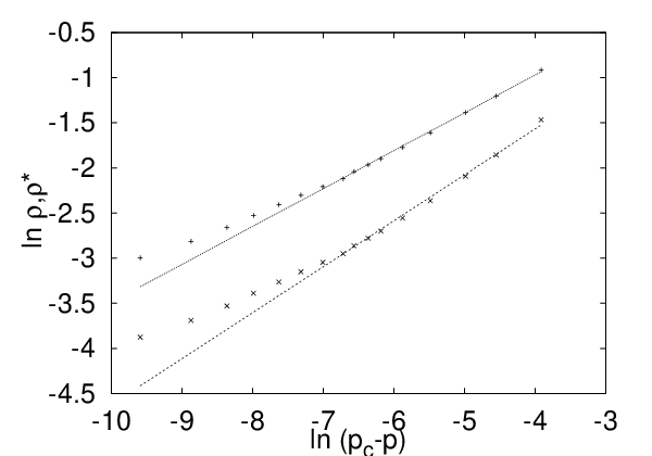
The value of can be determined by performing simulations at non-critical values of , where the system reaches its steady state. Here, we used simulations at constant density for this. The exponent can be extracted from a logarithmic plot of the density versus . Figure 2 shows such a plot. At higher densities, this yields values for which are consistent with earlier reported measurements, significantly higher than . However, it is clear that this fit does not hold up for the lower densities, which can be reached in the constant-density simulations. In addition, for the region with higher densities, the slopes for the particle and the pair density are clearly different, showing that an analysis consisting of a simple linear fit cannot be trusted.
For the calculation of the critical exponent we examine finite-size effects on a system at the critical value of . If the system size is small, these effects will cause the density to start decaying exponentially once the correlation length approaches the system size. Since the particle and pair densities are tied closely together, they will collapse at the same time. After sufficient time, the density will then decay as:
| (19) | |||||
| (20) |
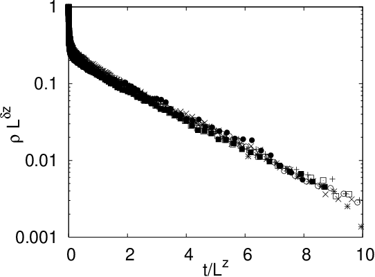
Using Eq. (20), the exponent can be obtained from simulations in small systems of various sizes until past this point of collapse, and adjusting the exponent until a data collapse can be attained for the exponential regime. We simulated systems for and 0.9, with system sizes ranging from to 5000 sites. For system sizes larger than this, the collapse occurs at late times, and therefore at a very low density. Apart from the very long simulation times, this poses another problem. To have accurate data at that point, we would have to know accurately enough such that its error obeys . With the density dropping below near the point of collapse for larger systems, would have to be smaller than to avoid significant systematical errors. Since our precision in is not that accurate, our range for the system size is limited by this effect.
At the time the density starts collapsing, . Since up to this point, the density was following a power law, we know that the density at this point will be . Using this, we can scale the data from our simulations to obtain a data collapse, as shown in Figure 3 for . It turns out that scaling the vertical axis works best with = , though the optimal value for in the horizontal scaling again varies with .
Table 2 shows the results for all exponents, for the three values of we investigated. The exponents all vary when the diffusion parameter changes, which, assuming PCPD falls into a single universality class, again points out there is something wrong with such a direct analysis.
| 0.1 | 0.1111 | 0.22 | 0.24 | 0.48 | 0.60 | 1.83 |
|---|---|---|---|---|---|---|
| 0.5 | 0.1524 | 0.19 | 0.20 | 0.42 | 0.51 | 1.75 |
| 0.9 | 0.2333 | 0.19 | 0.20 | 0.34 | 0.39 | 1.64 |
IV Analysis including corrections
Given the problems with the direct analysis of the critical exponents and , we propose introducing correction terms into our scaling laws. Both and obey the power laws as before, but with the DP values for the leading term in each relation, and an added correction term with a higher exponent. For the time-dependence of the density, this yields
While it is expected that the exponents for the two relations are the same, the prefactors for the particle density can be different from those for the pair density. This makes it possible to determine linear combinations of and where one of the two terms is suppressed, using
To determine all coefficients accurately, we will need both exponents. The correction exponent can be computed once a value for has been found that turns into a linear function of , at least for low densities. As a starting estimate for this ratio, an extrapolation of the ratio for can be used. Figure 4 shows the plots used to determine and calculate .

With the exponent known, and using the DP value for , it is now possible to fit both and with a linear combination of and , to obtain the prefactors and . These fits are shown for in Figure 5. The consistency of our fits can then be checked by determining and again from a linear fit to logarithmic plots of the appropriate linear combinations of and . In addition, the assumption for can be checked to make sure that it equals the ratio between the values from the fit.


Going through this process for , the final fit to determine from the computed ideal combination of and gives a value of 0.16(2), as shown in Figure 6, consistent with . The Figure also shows the effective exponent as it changes during the simulation. The remaining curvature in these graphs is sensitive to small changes in the estimation of , even if those do not significantly affect the resulting exponents. Therefore, this deviation from a straight line is most likely caused by an inaccuracy in this estimation. The differences between the estimated and calculated ratio and between the two obtained values for are well within the error margins for those values. In Table 3, the results for the fit are shown also for other values of .
| a | ||||||||
|---|---|---|---|---|---|---|---|---|
| 0.1 | 2.56 | 0.531 | 0.41 | 3.60 | 0.16 | 2.44 | 0.16(2) | 0.571 |
| 0.5 | 2.43 | 0.625 | 0.47 | 3.47 | 0.19 | 1.96 | 0.16(2) | 0.633 |
| 0.9 | 4.19 | 0.858 | 0.37 | 27.0 | 0.089 | 9.31 | 0.16(2) | 0.887 |
As seen in the table, the exponent seems to vary as changes. It is likely, however, that this is the effect of further correction exponents, whose coefficients depend on . Given the numerical precision of our data, it would be too optimistic to claim that our values for are accurate. A fit of Eq. (7) with to the high-quality data of Ref. hinr06, which runs up to time , yields correction exponents as low as . This shows that either the corrections to are very strong, or that the leading finite-time corrections actually cancel out in , causing us to measure the next correction exponent instead.
A similar process can be followed for determining , using the constant density simulations. Again, we used , with simulation times varying based on the relaxation time of the system. Our densities range from to . For low densities, it can take up to simulation steps until the system no longer shows a systematic drift. The assumed behavior of the densities is
Of course, the values for the prefactors, as well as the correction exponent, will be different from those in equations IV. However, the value for should still be the thermodynamic limit of the ratio , and thus will be the same as in our calculation of .
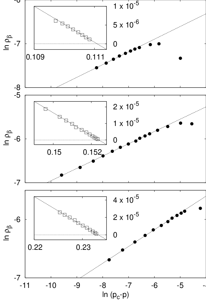
Plotting the linear combination of and which suppresses the leading term, using the same ratio of as before, we can determine the first correction exponent . With the exponents of the two leading terms known, we can again fit these to the data to determine their prefactors, and find the linear combination which will suppress the correction term. The result of this is shown in figure 7. Again, the values from the fit to cross-check and show that these estimates are consistent with the fit. Table 4 shows the results for different values of . Again, the correction exponent varies slightly as the diffusion parameter changes, suggesting additional corrections beyond the first. However, all data is consistent with a .
To confirm that we are performing our simulations at the critical point, we can calculate from these constant density simulations as well. With the same linear combination of the density and pair density as used for calculating , we again suppress the correction term. Since is a linear function of , and equals 0 at , finding is a matter of linear extrapolation, as shown in the insets in Figure 7. The results are in agreement with the values for used for all our simulations at the critical point, as seen in Table 4.
| a | ||||||||
|---|---|---|---|---|---|---|---|---|
| 0.1 | 1.058 | 0.62 | 43.1 | 0.24 | 26.5 | 0.29(3) | 1.055 | 0.1111 |
| 0.5 | 1.056 | 0.70 | 16.4 | 0.29 | 10.5 | 0.28(2) | 1.070 | 0.1524 |
| 0.9 | 1.270 | 0.43 | 17.0 | 0.10 | 7.77 | 0.29(3) | 1.285 | 0.2333 |
Lastly, we turn to the exponent . While the data collapse in figure 3 is acceptable, we do find different values of at and . Since we have demonstrated that equal values for the exponents and can be obtained for different values of by including correction terms, this encourages us to try out a similar approach here.
As before, we add a correction term to the relevant equation, in this case the one for the density during the collapse, and see how this fits with the DP exponents. The density will now decay differently, following:
| (32) |
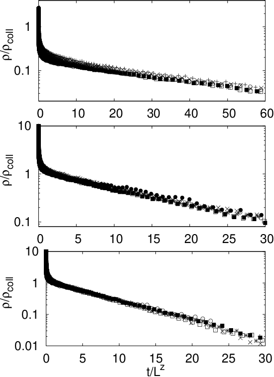
with an unknown constant and the correction exponent, with prefactor . Considering that one of the determining factors of the system is diffusion, where the correlation length grows as , a correction exponent of is a reasonable assumption. Sadly, with the range of data available it is impossible to determine this exponent accurately. We can, however, assume and , and show that this will provide data collapses at least as acceptable as the ones without a correction term. We use the same scaling as before, though we include the corrections calculated in our analysis for in our vertical scaling:
| (33) |
with , and taken from Table 3.
Note that there still is only one free parameter in our data collapse after these assumptions have been made: instead of varying the exponent , modifying the prefactor is now the only way to make the data from different system sizes overlap, both for the particle density and the pair density. This prefactor for the correction term can vary as changes, however. By plotting this relation for different sizes, we can find the value for that causes a data collapse, as well as the equivalents for the pair density. The ratio of the particle density and pair density varies very little in the regime we are examining here, and the point of collapse is equal for both, so we expect that and are equal. Fig. 8 shows the data collapses for three values of . While this does show that all of our data can be seen as consistent with , there is no clear way to show that this interpretation is better than the simpler approach, which yields varying exponents for different values of . However, it does seem more likely that if the other two exponents are independent of the diffusion rate, the same should hold for .
V Conclusion
Monte Carlo simulations, both the usual approach with constant rate and a new approach at constant density, have been used to analyze the critical behavior of the pair contact process with diffusion. While many recent studies conclude that this model does not belong to the directed percolation universality class, we find that if correction terms are included in the power laws governing critical scaling, all of the acquired simulation data is consistent with the exponents from DP.
In our simulations, especially the calculations for and offer convincing evidence that the DP values for these critical exponents are indeed accurate for the PCPD model. Since the critical exponents for and must be equal, any linear combination of these must have the same exponents as well, in the thermodynamical limit, except in the singular case where the leading terms cancel out. The fact that there exists a linear combination which follows a power law that is consistent with the DP exponent shows that the correct exponent for the system can at least not be any larger than that. Our analysis of does not lend itself to an accurate calculation of the exponent, but does also show that a correction term can explain the deviation from the DP exponent. With all of our simulation data consistent with DP for all three of the studied exponents, and for all investigated diffusion rates, we conclude it is likely that PCPD does belong to the directed percolation universality class.
We thank Haye Hinrichsen for providing us with the data described in Ref. hinr06.
References
- (1) H. Hinrichsen, Adv. Phys. 49, 815 (2000).
- (2) J. Marro and R. Dickman, Nonequilibrium phase transitions in lattice models (Cambridge University Press, Cambridge, UK, 1996).
- (3) M. Howard and U. Täuber, J. Phys. A: Math. Gen. 30, 7721 (1997).
- (4) P. Grassberger, Z. Phys. B, 47, 365 (1982).
- (5) H. K. Janssen, Z. Phys. B, 42, 151 (1981).
- (6) H. K. Janssen, F. van Wijland, O. Deloubrière and U. C. Täuber, Phys. Rev. E70, 056114 (2004).
- (7) S.-C. Park and H. Park, Phys. Rev. Lett. 94, 065701 (2005)
- (8) G. T. Barkema and E. Carlon, Phys. Rev. E68, 036113 (2003).
- (9) H. Hinrichsen, Physica A, 361,2 (2006).
- (10) J. Kockelkoren and H. Chaté, Phys. Rev. Lett. 90, 125701 (2003).
- (11) S. Kwon and Y. Kim, Phys. Rev. E75, 042103 (2007).
- (12) S.-C. Park and H. Park, Phys. Rev. E73, 025105(R) (2006)
- (13) K. Park and I. M. Kim, Phys. Rev. E66, 027106 (2002).
- (14) R. Dickman and M. A. F. de Menezes, Phys. Rev. E66, 045101(R) (2002).
- (15) G. Ódor, Phys. Rev. E67, 016111 (2003).
- (16) G. Ódor, Phys. Rev. E62, R3027 (2000).
- (17) E. Carlon, M. Henkel, U. Schollwöck, Phys. Rev. E63, 036101 (2001).
- (18) H. Hinrichsen, Phys. Rev. E63, 036102 (2001).
- (19) K. Park, H. Hinrichsen and I-M. Kim, Phys. Rev. E63, 065103(R) (2001).
- (20) J. D. Noh and H. Park, Phys. Rev. E69, 016122 (2004).
- (21) M. M. de Oliveira and R. Dickman, Phys. Rev. E74, 011124 (2006).
- (22) M. Henkel and H. Hinrichsen, J. Phys. A 37, R117 (2004).
- (23) J. Wallinga, Oikos 74, 377 (1995).
- (24) H.-M. Broeker and P. Grassberger J. Phys. A 267, 453 (1999).
- (25) H. J. Hilhorst and F. van Wijland, Phys. Rev. E65 035103(R) (2002).