CMB Temperature Polarization Correlation and Primordial Gravitational Waves II: Wiener Filtering and Tests Based on Monte Carlo SimulationsCMB Temperature Polarization Correlation and Primordial Gravitational Waves II: Wiener Filtering and Tests Based on Monte Carlo Simulations–Acknowledgments2007
Abstract
In this paper we continue our study of CMB TE cross correlation as a source of information about primordial gravitational waves. In an accompanying paper, we considered the zero multipole method. In this paper we use Wiener filtering of the CMB TE data to remove the density perturbation contribution to the TE power spectrum. In principle this leaves only the contribution of PGWs. We examine two toy experiments (one ideal and one more realistic), to see how well they constrain PGWs using the TE power spectrum. We consider three tests applied to a combination of observational data and data sets generated by Monte Carlo simulations: (1) Signal-to-Noise test, (2) sign test, and (3) Wilcoxon rank sum test. We compare these tests with each other and with the zero multipole method. Finally, we compare the signal-to-noise ratio of TE correlation measurements first with corresponding signal-to-noise ratios for BB ground based measurements and later with current and future TE correlation space measurements. We found that an ideal TE correlation experiment limited only by cosmic variance can detect PGWs with a tensor-to-scalar ratio at confidence level with the test, confidence level with the sign test, and confidence level for the Wilcoxon rank sum test. We also compare all results with corresponding results obtained using the zero multipole method. We demonstrate that to measure PGWs by their contribution to the TE cross correlation power spectrum in a realistic ground based experiment when real instrumental noise is taken into account, the tensor-to-scalar ratio, , must be approximately four times larger. In the sense to detect PGWs, the zero multipole method is the best, next best is the S/N test, then the sign test, and the worst is the Wilcoxon rank sum test.
Keywords:
cosmic microwave background – polarization – gravitational waves – cosmological parameters1 Introduction
Primordial gravitational waves (PGWs) (tensor) generate negative temperature-polarization (TE) correlation for low multipoles, while primordial density (scalar) perturbations generate positive TE correlation for low multipoles (see Crittenden et al. 1995; Baskaran et al. 2006; Grishchuk 2007; Polnarev et al. 2007; and references in Polnarev et al. 2007). This signature can be to detect PGWs. The test based on this signature (the zero multipole method, see Polnarev et al. 2007) is useful as an insurance against false detection or as a monitor of imperfectly subtracted systematic effects.
In this paper, we analyze an alternative method. This method uses Wiener filtering to remove the contribution of density perturbations to the TE cross correlation power spectrum for small , leaving only the negative residual component of the TE power spectrum due to PGWs. Actually, this method can be treated a test of the (negative) contribution to the TE correlation power spectrum due to PGWs on large scales using uncertainties in the measurements consistent with the total TE power spectrum. We use Monte Carlo simulations to analyze the probability of detecting PGWs using this method.
By detection of PGWs we mean in this paper, the measurement of the parameter , the ratio of the primordial tensor power spectrum, , to the primordial scalar power spectrum, , taken at wavenumber, :
| (1) |
where (see Smith et al. 2006). For this paper we only consider the tensor-to-scalar ratio, . All other parameters are assumed to be at their WMAP3 values (Spergel et al. 2007). The only other parameter which might affect the results is the tensor spectral index, , however we assume, in this paper, that is very close to zero (Peiris et al. 2003). The problem of will be considered in another paper.
The plan of this paper is the following. In Section 2, we describe the method for detection of PGWs based on measurements of the TE power spectrum. In Section 3, we describe the numerical Monte Carlo simulations we tested. In Sections 4, 5, and 6, we introduce the statistical tests used to contstrain PGWs. In Section 7, we compare the three different statistical tests used in this analysis. Section 8 gives the results for the two toy experiments described in Polnarev et al. 2007. The only uncertainty in the first toy experiment is due to cosmic variance (8.1). In the second toy experiment, along with cosmic variance, we take into account instrumental noise (8.2). We present results of Monte Carlo simulations for WMAP (8.3) and Planck (8.4). In Section 9, we compare signal-to-noise ratio for BB and TE measurements.
2 Wiener Filtering of the TE Cross Correlation Power Spectrum
Wiener filtering has been used often in the case of CMB data analysis. For example, it was used to combine multi-frequency data in order to remove foregrounds and extract the CMB signal from the observed data (Tegmark & Efstathiou 1996; Bouchet et al. 1999). Here we examine the use of the Wiener filter to subtract the PGW signal from the total TE correlation signal. This is done because the Wiener filter reduces the contribution of noise in a total signal by comparison with an estimation of the desired noiseless signal (Vaseghi 2006). In our case, the signal is the one due to PGWs only, and the signal contributed by density perturbations is considered to be “noise”.
The observed signal can be written as
| (2) |
where and refer to the contributions to the power spectrum due to scalar and tensor perturbations respectively. The values and refer to the spherical harmonic coefficients of the temperature and polarization maps. In our application to TE correlation, we consider the Wiener filter, :
| (3) |
The filtered signal, (for and ), is obtained from the measured signal, , as
| (4) |
In this paper, we assume the Wiener filter is perfect, in the sense that it leaves the signal due to PGWs only. We then get, for the filtered multipoles ,
| (5) | |||||
In practice this is not true, because we are trying to determine , which is not known in advance. Nevertheless, the assumption that the Wiener filter is perfect is good as a first approximation and illustrates the detectability of PGWs with the help of TE correlation measurements.
The filtering can reduce the measured signal to the desired signal, but, since we are trying to remove the density perturbations and not the actual noise, we can not reduce the measurement uncertainties. These uncertainties in are then entirely determined by the noise in the original signal.
From Polnarev et al. 2007, we showed that the TE power spectrum due to PGWs is negative on large scales, hence a test determining whether the Wiener filtered power spectrum is negative or not is a probe of PGWs.
There are three different statistical tests we use to see if we can measure a negative TE power spectrum. The first test is a Monte Carlo simulation to determine signal-to-noise ratio, (Section 4). The other two tests are standard non-parametric statistical tests: the sign test (Section 5) and the Wilcoxon rank sum test (Wilcoxon 1945) (Section 6).
3 Monte Carlo Simulation
For all of our tests, we calculate a random variable. If the data satisfies the hypothesis that , we can calculate the mean and uncertainty in the variables. If we make one realization of data, the random variable is determined from its distribution. Because we are not using any real observational data, we must run a Monte Carlo simulation to reduct the risk of randomly getting a value for the variable taken from the outlying area of its distribution. To do this, the filtered multipoles, , are randomly chosen from a gaussian distribution with mean and standard deviation where
| (6) | |||||
(see, for example, Dodelson 2003), the variable refers to the fraction of the sky covered by observations and is the effective power spectrum of the instrumental noise (see Dodelson 2003 for details on how is related to actual instrumental noise). The underlying power spectra are generated by CAMB11 1 see http://camb.info on web (Lewis et al. 2000).
Our determination of is dependent on . However, for two of our tests we ignore the value of in the calculation of the random variable. We assume that the calculated random variable is gaussian. In order for this to work, the random variable must be calculated from gaussian variables. Fig. 1 shows the combined distribution of the multipoles for the “ideal” toy experiment (see Section 8). To do this, for every we determine different values. We then combine all the different values, for every , into one large distribution. Fig. 1 shows the errors on the multipoles are large enough so that for our statistical tests we can assume the multipoles are taken from a single distribution and not from a distribution that depends on .

4 Monte Carlo S/N Test
For this test, the random variable we calculate, , is defined as
| (7) |
The reason why the sum in this equation is taken in the range is because only in this range . In other words, if we include higher multipoles we confront with a danger of a false detection, because the total TE power spectrum is negative for .
The value of is gaussian distributed because it is a sum of many modes of squares of gaussian distributed values, . We approximate each as being gaussian distributed for the purpose of this paper. For each set of parameters we run this simulation one million times to determine the mean, , and standard deviation, . The mean of this distribution is determined by the preassumed value of , while the standard deviation is determined by parameters of the experiment and gives the confidence level of detection. We run such Monte Carlo simulations for different values of to determine in what range of we can detect PGWs. When then using real observational data, we can compare the actual value of with the results of Monte Carlo simulations to infer the likelihood, as function of , which determines the probability that , or that PGWs exist at detectable levels.
5 Sign Test
The sign test is a test of compatability of observational data with the hypothesis that . If we do have , then will be equally distributed around zero. Application of this test to the filtered data is very simple. In practice, all observational data are distributed between several bins and the averaging of the signal is produced in each bin separately. Let be the number of such bins. The sign test actually gives the probability that in bins the average is negative and in it is positive, if . This probability, , is given by the binomial distribution
| (8) |
The probability that the hypothesis is wrong is
| (9) |
The value is the probability that we would get positive values given . This is the same as the probability of getting negative values given . Therefore our confidence that is just minus the sum of the probabilities describe above (the probability that the is closer to the mean, , if ). This equation only makes sense if , since that is required for . If , that would imply , which is not physical. We would have to interpret the result as a random realization of , with the most likely result of . Therefore we would not be able to say with any confidence.
Let us consider the following example: we put all measurements of into bins and in three of them the average is positive. In this example, the probability that the hypothesis is wrong is equal to .
One possible drawback of this method is that it does not take into account any measure of the signal-to-noise ratio of individual measurements. As we show in Section 7, it is possible to have two completely different sets of data with the same probability of having . This test is also unable to make any prediction as to the value of , only that it differs from zero.
6 Wilcoxon Rank Sum Test
This statistical test deals with two sets of data. The first set of data is taken from a real experiment which measures with some unknown . The second set of data is generated by Monte Carlo simulations (see Section 4) with . The objective of the Wilcoxon rank sum test is to give the probability that the hypothesis is wrong (Wilcoxon 1945).
First, we choose some random variable , whose probability distribution is known if . For that, let us combine all data from first set with multipoles and second set with multipoles into one large data set, which obviously contains multipoles. Then, we rank all multipoles in the large data set from to according to their amplitude (rank for the smallest and rank for the largest). Now, the variables and are defined as the sum of the ranks for the first original data set and the second original data set, correspondingly. Finally, the variable , is
| (10) |
If all multipoles of the first data set are larger than all multipoles of the second data set, then and . It is not difficult to show that . If both sets of measurements have no evidence for PGWs, . It is also simple to see that .
It is important to emphasize that the ranks of multipoles are random variables because all multipoles themselves are random variables, hence , , and are random variables. If is large, the distribution of can be approximated as a gaussian with a known mean and standard deviation. In this approximation we have
| (11) | |||||
| (12) |
In some cases, instead of , the variables or are used. The reason is used here is because is symmetric in the data sets. If in both sets of data, then the distributions of and are the same, no matter what and are. The distributions of and would be the same only if . The probability that the first data set corresponds to obtained from the test in which or is used is the same as if is used.
Since this test requires Monte Carlo simulations for the second set of data, we ran this test many times for many different data sets to get an accurate mean value for .
To reject the hypothesis means to detect PGWs. Using the Wilcoxon rank sum test the allowable value of is determined, if instead of comparing with simulated data with , we compare with simulated data with . In order to get a range of allowable values for , we need to run multiple Monte Carlo simulations with multiple values for . This is where the assumption that the are from a random distribution that is independent of is used (see Section 3). This implies that the ranks are random variables. If the errors on the are small enough, then the ranks will be predetermined. Therefore, our assumption about the distribution of will not be true and the test would have to be modified. Fortunately, this is not the case for even an experiment only limited by cosmic variance.
To illustrate how this test works, let us consider the following example. Assume there are multipoles in the first set of data and consider that is the correct value. There are also multipoles in the second set of data (which for sure corresponds to ). All quantities below are expressed in K2. The value for the first data set are , , , and . The values for the second data set are , , , and . A ranking of multipoles gives the ordering from lowest to highest, with referring to the first data set and referring to the second data set, as . This results in , , and . Therefore . For , to reject the hypothesis that at confidence level, should be less than one (see, for example, Lehmann 1975). In this example, since , the first set of data cannot be considered as a detection of PGWs.
7 Comparison of Tests
The test is greatly affected by outlying measurements. A measurement of one large negative multipole could falsely implay a detection. Both the sign test and the Wilcoxon rank sum test are not affected by individual outlying measurements. In the sign test, the value of individual measurements is irrelevant, because the test is sensitive only to the sign of individual measurements. The Wilcoxon rank sum test is affected by outliers, but considerably less than the test. If the outlier is larger (or smaller) than every other multipole, its rank does not depend on its particular value.
If we have two completely different sets of data, the main disadvantage of the sign test, as mentioned in Section 5, is that it could give the same result, while for the two other tests the chance to obtain the same value of is negligible. For example, one set of data, consisting of small negative multipoles and large positive multipoles, gives the same result as another set of data, consisting of large negative multipoles and small positive multipoles. The test gives two very different values of for these two sets of data. We can also use the Wilcoxon rank sum test to compare these two sets of data. In this case , which corresponds to a confidence level of hypothesis that of less than .
With observational data, the sign test can be applied and does not require any Monte Carlo simulations (which could be considered as an advantage of this test). The test requires Monte Carlo simulations, but only for the distribution of the random variable . The Wilcoxon rank sum test requires large Monte Carlo simulations and combines the data sets generated by these simulations with observational data. In other words, Monte Carlo simulations are absolutely necessary after obtaining observational data, which may be considered a disadvantage of this test. Thus, each of the three tests has advantages and disadvantages, suggesting that the best way to work out observational data is to apply all these three tests.
8 Discussion and Results
The current best limit of is at confidence provided by WMAP in combination with previous experiments (Spergel et al. 2007). We need to see if this method can detect a value of that is currently within the limit. We provide results for in order to see how well these tests can detect an amount of PGWs that is very close to being ruled out by BB measurements. For all our tests we assumed that there is no foreground contamination. For the experiments that are not observing the full sky, correlations between multipoles must be taken into account. We bin together the highly correlated multipoles so that the correlations between the bins are sufficiently small.
The two toy experiments that were used in Polnarev et al. 2007 are also used here to constrain . The two toy experiments are fully described in Polnarev et al. 2007, however we will also reproduce their description here.
The first toy experiment is a full sky experiement. For this experiment, we take measurements over the full sky with no instrumental noise. The only uncertainty will be due to cosmic variance. This experiment represents the best limit to which the gravitational waves can be detected with the TE correlation. A space-based experiment with access to the full sky is the closest to this experiment. It is similar to what the Beyond Einstein inflation probe will be able to detect. This toy experiment will be hereafter referred to as the ideal experiment.
The second toy experiment is a more realistic experiment. Measurements of the CMB are taken on of the sky in one frequency ( GHz) for years. The noise in each detector of the polarization sensitive bolometer pairs can be described by their noise equivalent temperature (NET) of . The detector beam profiles are assumed to be gaussian and and it is described by their full width half maximum (FWHM) of .
This second toy experiment is similar to current ground-based experiments. Constraints from this experiment represent those that can and will be obtained in the next several years using this method. This will be referred to as the realistic experiment.
We also look at experiments with instrumental noise similar to the satellite experiments WMAP and Planck. The predicted errors for Planck are based on using the GHz, GHz, and GHz channel in the High Frequency Instrument (HFI). The numbers are gotten from the Planck science case, the ‘‘bluebook’’22 2 http://www.rssd.esa.int/index.php?project=Planck. The WMAP noise was obtained by using years of the Q-band, V-band, and W-band detectors.
8.1 Ideal Experiment
A plot of the TE power spectrum due to PGWs for and for the ideal experiment is shown in Fig. 2. The errors bars in Fig. 2 are calculated from the total TE power spectrum. There are no correlations between multipoles, because we observe the full sky, but we plot the error bars binned in intervals of for simplicity in the plot.

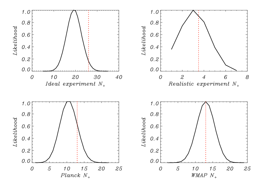
The Monte Carlo simulation gives an average of measured TE power spectrum multipoles greater than zero out of a total of independent multipoles. If the null hypothesis was true, the sign test would indicate there is a chance of measuring positive multipoles. This is equivalent to a detection. A plot of the distribution of the number of positive multipoles is shown in the upper panel plot of Fig. 3. There is an chance for the observed to give a detection of PGWs.
The test gives a mean value of and standard deviation of . The upper left panel in Fig. 4 shows the distribution of the values for the Monte Carlo simulation with . If we would have a probability of the measured . This negative value signifies that a non-zero tensor-to-scalar ratio produced an anti-correlation. We can assume that the standard deviation would be the same if the mean of was (equivalent to ), because it is equivalent to adding a constant value to every measured value (and hence adding a constant to which would not change the error). Therefore, if , the probability of getting is , and hence we have a chance that . A plot of and as a function of is shown in Fig. 5. As can be seen from the plot, we can predict a value of for any value of . The value of is a relatively constant function of and so our prediction about the distribution of for different value of is a good approximation to the true distribution.


The Wilcoxon rank sum test gives . The variable is the mean value for in the Monte Carlo simulations described earlier. The values and are given in Section 6. The distribution of for the Monte Carlo simulations with is shown in Fig. 6. The standard deviation of the distribution of measured is the same as the standard deviation of the distribution of assuming the hypothesis that . The only difference between the distributions is that is shifted by a constant value. Therefore, there is a chance that . There is also a chance that we measure , and are not even able to make a detection of PGWs.

A comparison of the three tests is shown in Fig. 7. This is obtained by simulated with with several values of and then interpolating between them. A detection is obtained for ( test), (sign test), and (Wilcoxon rank sum test), highlighting its intended use as a monitor of a false positive detection for large .

8.2 Realistic Ground Based Experiment
A plot of the TE power spectrum due to PGWs with is shown in Fig. 8. The error bars are calculated from the total TE power spectrum. Observations of an incomplete sky require the multipoles to be binned in sizes of . This experiment has much larger error bars than the ideal experiment and it will not be able to detect low values of with the TE cross correlation only.

The results for the Wiener filtering method were much worse than those for the ideal experiment for . Since this experiment observes a small portion of the sky, the multipoles are correlated and we must bin together to get reasonably uncorrelated measurements. For this experiment, we only have to uncorrelated multipoles, instead of uncorrelated multipoles in the case where the full sky is observed. Getting out of negative multipoles is a probability if there are no PGWs. For the Monte Carlo simulations of the realistic experiment, on average, half of measured multipoles are positive and half are negative. A plot of the distribution of the number of positive multipoles is shown in the upper right panel of Fig. 3. In this case, we cannot distinguish from with any significance.
The test gives an average value of with standard deviation of . For the realistic toy experiment, the distribution of for is shown in the upper right panel of Fig. 4. In order to obtain confidence detection of PGWs, we must use . In this sense the TE test provides monitoring and insurance against false positive detection with , which could arise, for example, if foregrounds or other systematic effects arer improperly removed.
The last statistical test, the Wilcoxon rank sum test, gives . The distribution of for is shown in the upper right panel of Fig. 6. This gives the weakest result in terms of the three tests for the Wiener filtered data. The realistic experiment will not be able to constrain using the TE cross correlation power spectrum. Its limit is closer to at only confidence depending on the test used. For a higher confidence in a detection of PGWs, the value of would need to be much higher. Since the observed distribution of corresponds almost exactly to the simulated distribution of under the assumption that , therefore we have a chance of measuring .
8.3 WMAP
The results of the Wiener filtering showed that the WMAP cannot make a detection of gravitational waves using the TE cross correlation power spectrum alone. As with the two toy experiments, the result of the scalar and tensor separation was similar. The Monte Carlo simulation gave on average gave positive multipoles out of a total of uncorrelated multipoles. We would get the same result if the input data had so we cannot detect PGWs with WMAP using only the TE power spectrum. A plot of the distribution of the number of positive multipoles is shown in the lower right panel of Fig. 3. As can be seen, this distribution of for WMAP noise and is simply the distribution for .
For WMAP, the S/N test gives the value of with a standard deviation of . The distribution is shown in the lower right panel of Fig. 4. The distribution is centered around so there is no chance of using this test to detect PGWs in WMAP’s TE power spectrum. The probability of getting a or detection is the same probability that we would randomly get a detection if there are no PGWs.
The rank sum test gives a value of , which is implies no ability to distinguish WMAP’s observed TE data from a data set with no PGWs. A plot of the distribution of for WMAP error bars is shown in the lower right panel of Fig. 6. We reach the same conclusion for WMAP noise as for the realistic experiment. There is only a chance that we can measure and make a detection of
The published WMAP results show an anti-correlation of TE power spectrum at large scales. Unfortunately this is not a detection of PGWs as theorized in Baskaran et al. 2006. The contribution to the TE power spectrum due to PGWs only changes sign once for . If a claimed evidence for gravitational waves is to be believed, then the TE power spectrum would have to change sign three times for . In fact, other than the two anticorrelations at low , the rest of the multipoles, up to , are consistent with . None of the described tests applied to the current WMAP data will give any detection of PGWs.
8.4 Planck
The sign test gives on average positive measurements of the TE power spectrum out of a total of uncorrelated multipoles. There is a chance of getting positive multipoles if . A plot of the distribution of the number of positive multipoles for Planck is shown in the lower left panel of Fig. 3. There is a chance that we will measure and hence have a detection of .
The test gives a value of with a standard deviation of . There is only a chance that the test results in a value of larger than zero, if , and a chance getting if . This is close to a probability of detection. The distribution of the variable is shown in lower left panel of Fig. 4.
Again, the rank sum test gives the lowest confidence result with a value of . A plot of the distribution of is shown in the lower left panel of Fig. 6. There is a probability that we will measure and a probability that we measure for Planck.
9 Comparison of Measurements of TE Power Spectrum with BB Power Spectrum
CMB polarization can be separated into two distinct components: E-mode (grad) polarization and B-mode (curl) polarization. PGWs generate B-mode polarization in contrast to density perturbations (see for example Seljak 1997; Seljak & Zaldarriaga 1997; Kamionkowski & Kosowsky 1998). Therefore, most CMB polarization experiments searching for evidence of PGWs focus on measuring the BB power spectrum (see Taylor et al. 2004; Bowden et al. 2004; Yoon et al. 2006). For different aspects of CMB polarization generated by PGWs see, for example, Basko & Polnarev 1980; Polnarev 1985; Crittenden et al. 1993; Frewin et al. 1994; Coles et al. 1995; Kamionkowski et al. 1997; Seljak 1997; Seljak & Zaldarriaga 1997; Kamionkowski & Kosowsky 1998; Baskaran et al. 2006; Keating et al. 2006.
We have shown that the TE cross correlation power spectrum offers another method of detecting PGWs (Crittenden et al. 1995). The TE power spectrum is two orders of magnitude larger than the BB power spectrum and it was originally suggested that it might be easier to detect gravitational waves in the TE power spectrum than using the BB power spectrum (Baskaran et al. 2006; Grishchuk 2007). However, as we have shown in Polnarev et al. 2007, that, when we use zero multipole method, uncertainties in TE measurements exceed uncertainties in BB measurements in such a way that the signal-to-noise ratio for BB measurements is better than for TE measurements. We show below that the same is true for the separation of scalars and tensors.
However, an advantage of TE measurements for ground based experiments, which observe only a small fraction of the sky, is related to the fact that the main spurious effects in the BB power spectrum are cuased by E/B mixing. This will limit the that can be detected (Challinor & Chon 2005). The E-modes are practically unaffected by E/B mixing, so, in contrast to the BB measurements, the TE power spectrum should be nearly the same for both full and partial sky measurements.
Along with this, the methods based on the TE cross correlation can be considered as very useful auxiliary measurements of PGWs, because systematic effects in TE measurements are independent from those in BB measurements. For example, T/B leakage or even E/B leakage could swamp a detection of BB, whereas T/E leakage would be small and well controlled (see Shimon et al. 2007). These BB systematics could falsely imply a large , but measurements of the TE power spectrum provide insurance against such a spurious detection. Additionally, galactic foreground contamination will affect BB and TE in different ways, which enable us to perform powerful cross-checking and subtraction of foregrounds in BB measurements.
For the zero multipole method, we explained why the signal-to-noise ratio for BB measurements is better than for TE measurements. Below we give simple summarizing arguments why the same is true for the Wiener filtering of the TE power spectrum.
If , the signal-to-noise ratio for the BB power spectrum is
| (13) |
where
| (14) |
If then we will not be able to detect PGWs and a comparison with the TE power spectrum is not worthwhile.
If and , for the TE power spectrum, the signal-to-noise ratio is
| (15) | |||||
where and are
| (16) |
where
| (17) |
One can see that and are on the order of unity. Therefore, the signal-to-noise ratio is approximated as
| (18) |
In other words if , BB measurements have the obvious advantage in comparison with the Wiener filtering of the TE power spectrum. Indeed if , , while . This is because in BB measurements, applying proper data analysis, we can entirely eliminate contributions of scalar perturbations to CMB polarization signal as well as to the uncertainties. For the perfect Wiener filtering of the TE power spectrum, we can eliminate the contribution of scalar perturbations to the signal only, but cannot eliminate their contribution to the uncertainties.
10 Conclusion
The method described here is one in which we filter out the signal due to density perturbations, leaving only the contribution to the TE power spectrum due to PGWs. We then test the resulting TE power spectrum to see if it is negative. Three different statistical tests were used to see if there was a significant detection of PGWs. The test can give a value for using a comparison with Monte Carlo simulations, while the Wilcoxon rank sum test can only give an allowable range for . The sign test will only tell us if .
From Polnarev et al. 2007, we saw that we could detect to with a measure of , the position where the TE power spectrum first changes sign, for the ideal experiment. Using the method discussed in this paper, we see that we are unable to make this significant of a detection. The best result was for the test which would give a detection of . To detect PGWs on the level of , the tensor-to-scalae ratio should be . The sign test would give detection for and a detection for . The Wilcoxon ranked sum test gives only a detection for and a detection for . Similar results were gotten for the other three experiments tested. Thus in the sense of potential to detect PGWs, the zero multipole method is the best, next best is the test, then the sign test, and the worst is the Wilcoxon ranked sum test.
Baskaran et al. 2006 present illustrative examples in which high is consistent with measured TT, EE, and TE correlations. The value of is so high in these examples that if PGWs with such really existed, current BB experiments would already detect PGWs. All models predict that the TE cross correlation power spectrum change sign only once for . The fact WMAP cannot exclude several multipoles with in between multipoles of means that the TE cross correlation power spectrum either changes sign several times for or there is some instrumental noise which causes some anticorrelation measurements. Using instrumental noise consistent with WMAP, our Monte Carlo simulations give and , which means that there is no evidence of PGWs in the TE correlation power spectrum.
Acknowledgments
NJM would like to thank the Astronomy Unit, School of Mathematical Science at Queen Mary, University of London for hosting him while working on this paper. We acknowledge helpful comments on this manuscript by Kim Greist and Manoj Kaplinghat. BGK gratefully acknowledges support from NSF PECASE Award AST-0548262. We acknowledge using CAMB to calculate the power spectra in this work.
References
- Baskaran et al. (2006) Baskaran D., Grishchuk L. P., Polnarev A. G., 2006, Phys. Rev. D, 74, 083008
- Basko & Polnarev (1980) Basko M. M., Polnarev A. G., 1980, MNRAS, 191, 207
- Bouchet et al. (1999) Bouchet F. R., Prunet S., Sethi S. K., 1999, MNRAS, 302, 663
- Bowden et al. (2004) Bowden M., et al., 2004, MNRAS, 349, 321
- Challinor & Chon (2005) Challinor A., Chon G., 2005, MNRAS, 360, 509
- Coles et al. (1995) Coles P., Frewin R. A., Polnarev A. G., 1995, LNP Vol. 455: Birth of the Universe and Fundamental Physics, 455, 273
- Crittenden et al. (1993) Crittenden R., Davis R. L., Steinhardt P. J., 1993, ApJL, 417, L13+
- Crittenden et al. (1995) Crittenden R. G., Coulson D., Turok N. G., 1995, Phys. Rev. D, 52, 5402
- Dodelson (2003) Dodelson S., 2003, Modern cosmology. Modern cosmology / Scott Dodelson. Amsterdam (Netherlands): Academic Press. ISBN 0-12-219141-2, 2003, XIII + 440 p.
- Frewin et al. (1994) Frewin R. A., Polnarev A. G., Coles P., 1994, MNRAS, 266, L21+
- Grishchuk (2007) Grishchuk L. P., 2007, arXiv:0707.3319 [astro-ph], 707
- Kamionkowski & Kosowsky (1998) Kamionkowski M., Kosowsky A., 1998, Phys. Rev. D, 57, 685
- Kamionkowski et al. (1997) Kamionkowski M., Kosowsky A., Stebbins A., 1997, Physical Review Letters, 78, 2058
- Keating et al. (2006) Keating B. G., Polnarev A. G., Miller N. J., Baskaran D., 2006, International Journal of Modern Physics A, 21, 2459
- Lehmann (1975) Lehmann E. L., 1975, Nonparametric Statistical Methods Based on Ranks. McGraw-Hill
- Lewis et al. (2000) Lewis A., Challinor A., Lasenby A., 2000, ApJ, 538, 473
- Peiris et al. (2003) Peiris H. V., et al., 2003, ApJS, 148, 213
- Polnarev (1985) Polnarev A. G., 1985, SvA, 29, 607
- Polnarev et al. (2007) Polnarev A. G., Miller N. J., Keating B. G., 2007, arXiv:0710.3649 [astro-ph], 710
- Seljak (1997) Seljak U., 1997, ApJ, 482, 6
- Seljak & Zaldarriaga (1997) Seljak U., Zaldarriaga M., 1997, Physical Review Letters, 78, 2054
- Shimon et al. (2007) Shimon M., Keating B., Ponthieu N., Hivon E., 2007, arXiv:0709.1513 [astro-ph]
- Smith et al. (2006) Smith T. L., Kamionkowski M., Cooray A., 2006, Phys. Rev. D, 73, 023504
- Spergel et al. (2007) Spergel D. N., et al., 2007, ApJS, 170, 377
- Taylor et al. (2004) Taylor A. C., Challinor A., Goldie D., Grainge K., Jones M. E., Lasenby A. N., Withington S., Yassin G., Gear W. K., Piccirillo L., Ade P., Mauskopf P. D., Maffei B., Pisano G., 2004, arXiv:astro-ph/0407148
- Tegmark & Efstathiou (1996) Tegmark M., Efstathiou G., 1996, MNRAS, 281, 1297
- Vaseghi (2006) Vaseghi S. V., 2006, Advanced Digital Signal Processing and Noise Reduction. John Wiley & Sons
- Wilcoxon (1945) Wilcoxon F., 1945, Biometrics Bulletin, 1, 80
- Yoon et al. (2006) Yoon K. W., et al., 2006, in Millimeter and Submillimeter Detectors and Instrumentation for Astronomy III. Edited by Zmuidzinas, Jonas; Holland, Wayne S.; Withington, Stafford; Duncan, William D.. Proceedings of the SPIE, Volume 6275, pp. 62751K (2006). Vol. 6275 of Presented at the Society of Photo-Optical Instrumentation Engineers (SPIE) Conference, The Robinson Gravitational Wave Background Telescope (BICEP): a bolometric large angular scale CMB polarimeter