Dynamical quark recombination in ultrarelativistic heavy-ion collisions and the proton to pion ratio
Abstract
We study quark thermal recombination as a function of energy density during the evolution of a heavy-ion collision in a numerical model that reproduces aspects of QCD phenomenology. We show that starting with a set of free quarks (or quarks and antiquarks) the probability to form colorless clusters of three quarks differs from that to form colorless clusters of quark-antiquark and that the former has a sharp jump at a critical energy density whereas the latter transits smoothly from the low to the high energy density domains. We interpret this as a quantitative difference in the production of baryons and mesons with energy density. We use this approach to compute the proton and pion spectra in a Bjorken scenario that incorporates the evolution of these probabilities with energy density, and therefore with proper time. From the spectra, we compute the proton to pion ratio and compare to data at the highest RHIC energies. We show that for a standard choice of parameters, this ratio reaches one, though the maximum is very sensitive to the initial evolution proper time.
pacs
25.75.-qAugust 11, 2026
I Introduction
The features of the proton to pion ratio for Au + Au collisions at the highest energy at RHIC PHENIXBM have been interpreted as the emergence of thermal recombination as an important mechanism for hadron production in this environment. Recall that in p + p collisions, the proton to pion ratio as a function of remains basically unchanged, never exceeding one, for collision energies ranging from 19.4 GeV at the Tevatron, 44.6 and 52.8 GeV at ISR up to 200 GeV at RHIC STAR. This stable behavior with collision energy can be understood as a manifestation of the fact that in p + p collisions, hadron production is dominated by parton fragmentation and the proton to pion ratio simply reflects the ratio of the corresponding fragmentation functions. In contrast, the proton to pion ratio in collisions of heavy systems grows with collision energy Laszlo; STAR2, reaching and even exceeding one in Au + Au collisions at GeV for GeV/c. While it is possible to understand the different behaviors of the above ratios in collisions of heavy systems as partially arising from the increase of radial flow with collision energy ayala1; ayala2, another important ingredient that needs to be understood is how these ratios are influenced by the relative abundance of protons and pions when these particles are produced in the collision of heavy systems at the highest energies.
In its simplest form, the recombination scenario explains the formation of low to intermediate hadrons from the bounding of quarks in a densely populated phase space, assigning appropriate degeneracy factors for mesons and baryons recomb; Fries. However, it only accounts for correlations among quarks in momentum space but misses describing the corresponding expected correlation in coordinate space. An implicit assumption is that hadronization happens at a single temperature. However, it is known that hadronization is not an instantaneous process but rather that it spans a window of temperatures and densities. For instance lattice calculations Karsch show that the phase transition from a deconfined state of quarks and gluons to a hadron gas is, as a function of temperature, not sharp. The question that arises is to what extent the probability to recombine quarks into mesons and baryons depends on density and temperature and whether this probability differs for hadrons with two and three constituents, that is to say, whether the relative population of baryons and mesons can be attributed not only to the degeneracy factors but rather to the dynamical properties of quark clustering in a varying density scenario.
The detailed answer to the above question is a subject that belongs to the realm of confinement phenomena and thus to the dynamics of non-perturbative QCD. It is however possible to also address it in the context of numerical models that reproduce aspects of QCD phenomenology such as quark clustering at low density and color deconfinement at high density. One of such models is the so called string-flip model stringflip which has proven to be successful in the study of quark/hadron matter as a function of density string1; Genaro1; Genaro2. Other approaches toward a dynamical description of recombination, in the context of fluctuations in heavy ion collisions, have been recently formulated in terms of the qMD model 0702188.
In this work we compute the meson and baryon thermal spectra from a dynamical model of quark recombination. The work is organized as follows: In Sec. II, we introduce the formalism to incorporate the probability to form clusters of two and three quarks as a function of density and temperature in the description of thermal particle spectra. In Sec. III we present the basics to implement the numerical simulations in the string-flip model. In Sec. IV we use this model to compute the probability to form mesons and baryons from liberated quarks. In Sec. V we use these spectra to compute the proton to pion ratio and compare the results to experimental data. We finally present our conclusions and give an outlook in Sec. VI.
II Thermal Spectra
In general, the invariant transverse momentum distribution of a given hadron can be written as an integral over the freeze-out, space-time hypersurface of the relativistically invariant phase space particle density ,
| (1) |
where is the hadron’s momentum and is a future oriented unit four-vector normal to and is the degeneracy factor for the hadron which takes care of the spin degree of freedom.
In the recombination model, the phase space particle density is taken as the convolution of the product of Wigner functions for each hadron’s constituent quark at a given temperature and the constituent quark wave function inside the hadron. For instance, the meson phase space distribution is given by
| (2) | |||||
where is the light-cone momentum, is the meson wave function and represent the quantum numbers (color, spin, flavor) of the constituent quark and antiquark in the meson, respectively. An analogous equation can also be written for baryons. When each constituent quark’s Wigner function is approximated as a Boltzmann distribution and momentum conservation is used, the product of Wigner functions is given by a Boltzmann-like factor that depends only on the light-cone momentum of the hadron Fries. For instance, in the case of mesons
| (3) | |||||
In this approximation, the product of parton distributions is independent of the parton momentum fraction and the integration of the wave function over is trivially found by normalization. There can be corrections from a dependence of each constituent quark Wigner function on momentum components that are not additive because energy is not conserved in this scenario Fries2. The QCD dynamics between quarks inside the hadron is encoded in the wave function.
In order to allow for a more realistic dynamical recombination scenario let us take the above description as a guide, modifying the ingredients that account for the QCD dynamics of parton recombination. Let us assume that the phase space occupation can be factorized into the product of a term containing the thermal occupation number, including the effects of a possible flow velocity, and another term containing the system energy density driven probability of the coalescence of partons into a given hadron. We thus write the analog of Eq. (2) as
| (4) |
where is the flow velocity.
To compute the probability let us consider a model that is able to provide information about the likelihood of clustering of constituent quarks to form hadrons from an effective quark-quark interaction. We will explicitly consider the so called string-flip model which we proceed to describe.
III String Flip Model
The String Flip Model is formulated incorporating a many-body quark potential able to confine quarks within color-singlet clusters stringflip. At low densities, the model describes a given system of quarks as isolated hadrons while at high densities, this system becomes a free Fermi gas of quarks. For our purposes, we consider up and down flavors and three colors (anticolors) quantum numbers. Our approach is very close to that described in Refs. string1 and Genaro1, where we refer the reader for an extensive discussion of the model details. For completeness, here we describe the basic ingredients.
III.1 Many-body potential
The many-body potential is defined as the optimal clustering of quarks into color-singlet objects, where by optimal we mean the configuration that minimizes the potential energy. In our approach, the interaction between quarks is pair-wise. Therefore, the optimal clustering is achieved by finding the optimal pairing between two given sets of quarks of different color for all possible color charges.
Consider, for example, a set of quarks some with color and others with color , irrespective of flavor, in accordance to the the flavor-blindness nature of QCD. We define the optimal pairing between and quarks as:
| (5) |
where is the spatial coordinate of the -th quark and is the coordinate of the mapped -th quark. The minimization procedure is performed over all possible ! permutations of the quarks and the interaction between quarks (v) is assumed to be harmonic:
| (6) |
where is the spring constant. Through this procedure, we can distinguish two types of hadrons:
i) Meson-like. In this case the pairing is imposed to be between color and anticolors and the many-body potential of the system made up of mesons is given by:
| (7) |
where the individual terms are given by Eq. 5 for the corresponding colors. , and are the labels for red, blue and green color (anticolor) respectively. Note that this potential can only build pairs.
ii)Baryon-like. In this case the pairing is imposed to be between the different colors in all the possible combinations. In this manner, the many-body potential is:
| (8) |
which can build colorless clusters by linking 3(RBG), 6(RBGRBG),… etc., quarks. Since the interaction is pair-wise, the 3-quark clusters are of the delta (triangular) shape.
According to QCD phenomenology, the formed hadrons should interact weakly due to the short-range nature of the hadron-hadron interaction. This is partially accomplished by the possibility of a quark flipping from one cluster to another. At high energy density, asymptotic freedom demands that quarks must interact weakly. This behavior is obtained once the average inter-quark separation is smaller than the typical confining scale.
The Hamiltonian for the system built up of quarks of mass and momentum is given by:
| (9) |
In this work, as a first approach, we will study the meson and baryon like hadrons independently. Therefore, or , depending on the type of hadrons we wish to describe.
III.2 The variational wave function
We use a variational Monte Carlo approach to describe the evolution of a system of quarks as a function of the particle density. We consider the quarks moving in a three-dimensional box whose sides has length a and the system described by a variational wave function of the form:
| (10) |
where is the single variational parameter, (x1,…,xN) is the many-body potential defined in Eqs. (7) and (8) for mesons and baryons respectively, and (x1,…,xN) is the Fermi-gas wave function given by a product of Slater determinants, one for each color-flavor combination of quarks. These are built up from single-particle wave functions describing a free particle in a box Genaro1. The selection of the variational wave function rests in the fact that we are interested in the evolution of the system from low to high energy densities. The exponential term is responsible of the clustering correlations. At low energy density, the system is formed by isolated color-singlet hadrons and quarks strongly interact inside each cluster; in this case, the exponential term of the wave function has a big contribution since the average interquark distance is of the order of the confining scale. In contrast, at high energy density, where asymptotic freedom takes place, the interaction between quarks is weak and the system looks like a Fermi gas of quarks. In this case, the inter-quark separation is much smaller than the confining scale and the exponential term effect vanishes.
As we will show below, the variational parameter changes from a fixed value at low energy density (isolated clusters) to zero at high energy density (Fermi gas).
III.3 Variational Monte Carlo Calculations
We need to evaluate the expectation value of the Hamiltonian operator given by Eq. (9) and minimize it with respect to the variational parameter
| (11) |
In order to do this, we can take advantage of the structure of the wave function in Eq. (10), which allows some simplifications in the calculations. After an integration by parts, the expectation value of the Hamiltonian operator for a given particle density can be evaluated as:
| (12) |
where is the kinetic energy of a free Fermi gas, is the potential energy as defined by Eqs. (7) and (8) and is the term that indicates how the kinetic energy increases due to clustering correlations. This last is expressed as:
| (13) |
where the sum is over all quarks in the system and yi represents the average position of the two quarks connected to the -th quark for a baryon-like hadron or the corresponding antiquark position for a meson-like hadron.
A very important property of having written the expectation value as in Eqs. (12) and (13) is that the two functions to be evaluated ( and ) are local; consequently, their expectation values can be calculated using Monte Carlo techniques, in particular we use the Metropolis method to do the sampling. Finally, this procedure is carried out for different values of the particle density.

The variational parameter has definite values for the extreme density cases. At very low density it must correspond to the wave function solution of an isolated hadron. For example, the non-relativistic quark model for a hadron consisting of 2 and 3 quarks, bound by a harmonic potential, predicts, in units where that and respectively; at very high densities the value of must vanish for both cases. In the appendix, we show how to convert from the system of units where to physical units.
IV Probabilities
All the results we present here come from simulation done with 384 particles, 192 quarks and 192 antiquarks, corresponding to having 32 plus 32 quarks (antiquarks) in the three color charges (anti-charges).
To determine the variational parameter as a function of density we proceed as follows: first we select the value of the particle density in the box, which, for a fixed number of particles, means changing the box size. Then we compute the energy of the system as a function of the variational parameter using the Monte Carlo Method described in the previous section. The minimum of the energy determines the optimal variational parameter. We repeat the procedure for a set of values of the particle densities in the region of interest. In fig. 1 we exemplify the behavior of the energy per particle from the simulation (symbols) as a function of the variational parameter at low density () for a baryon system. The solid line is a fit to the data. We can observe that the expected values from the solution to the 3-quark system with a harmonic potential are properly approached. This is taken as an indication of the range where the value of the variational parameter should lay for an isolated hadron.
In order to check whether the variational approach describes the expected results in the low and high density limits, we display in fig. 2 the energy density dependence of the variational parameter for the baryon, , (triangle symbols) and meson, , (circle symbols) cases. In both cases, the behavior of the optimal parameter is the expected one, as described in detail in the previous section. At low densities, converges to the theoretical value ( and ) for baryons and mesons respectively. We use these to normalize the data such that the values for low energy densities is around 1; at high densities the values of both and approaches zero asymptotically. Nevertheless, there are differences between the two cases. In the case of baryons, there is a deep drop around 0.7 GeV/fm3 indicating that the length scale for quark confinement has increased in the medium (this unexpected behavior was also reported in Refs. Genaro1; string1), to subsequently evolve into the Fermi gas domain. For a meson system, the variational parameter has a smooth drop. The above indicates a qualitative difference in the formation of baryon and meson clusters, as a function of the energy density.
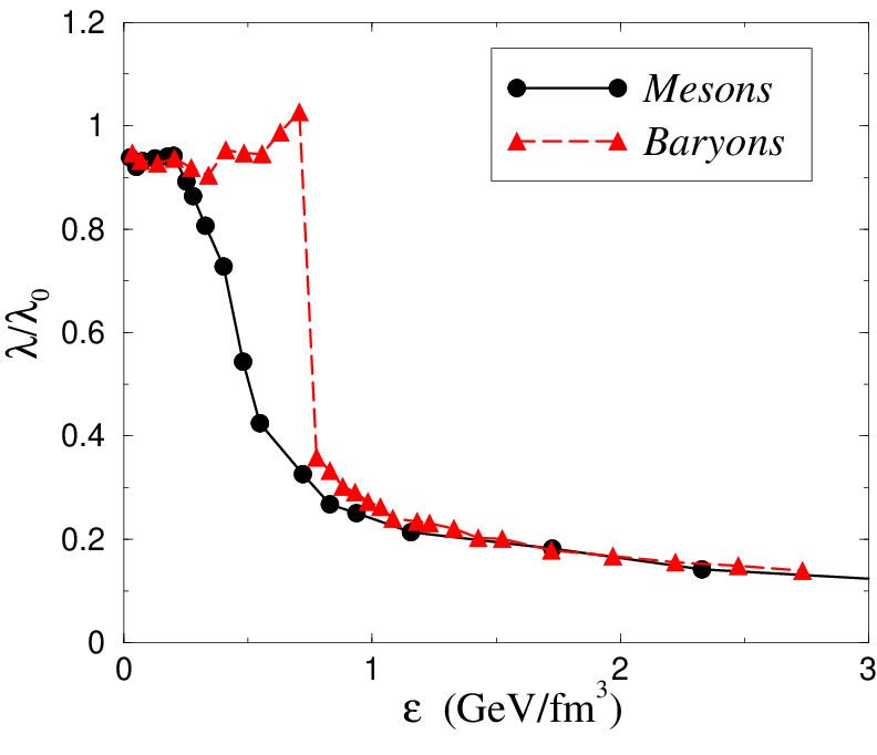
The information contained in the variational parameter is global, in the sense that it only gives an approximate idea about the average size of the inter-particle distance at a given density, which is not necessarily the same for quarks in a single cluster. This is reflected in the behavior of the variational parameter for the case of baryons which, from fig. 2, goes above 1 for energies close to where the sudden drop in the parameter happens. We interpret this behavior as as a consequence of the procedure we employ to produce colorless clusters for baryons, which, as opposed to the case to form mesons, allows the formation of clusters with a number of quarks greater than 3. When including these latter clusters, the information on their size is also contained in . To correct for this, we compute the likelihood to find clusters of 3 quarks . Recall that for quarks in the system, the total number of clusters of 3 quarks that can be made is equal to . However this is not always the case as the density changes, given that the potential allows the formation of clusters with a higher number of quarks. is defined as the ratio between the number of clusters of 3 quarks found at a given density, with respect to . This is displayed in fig. 3.
Therefore, within our approach, we can define the probability of forming a baryon as the product of the parameter times , namely
| (14) |
For the case of mesons, since the procedure only takes into account the formation of colorless quark-antiquark pairs, we simply define the probability of forming a meson as the value of the corresponding normalized variational parameter, namely
| (15) |
The probabilities and as a function of the energy density are displayed in fig. 4. Notice the qualitative differences between these probabilities. In the case of baryons, the sudden drop found in the behavior of the variational parameter is preserved at an energy density around GeV/fm3 whereas in the case of mesons, this probability is smooth, indicating a difference in the production of baryons and mesons with energy density.

These are the probabilities we set originally ourselves to look for and that we use in sec V to compute the proton to pion ratio. Before proceeding to that analysis, it is also instructive to learn more about the behavior of other properties of the quark system with energy density.
IV.1 Clusters’ size
To obtain a more precise information about the clusters’ size, we can look at the distribution of particles into a cluster, characterized by a mean square radius (MSR). To do so, we proceed to calculate the frequency distribution of clusters with a given value of the MSR. For the baryon system, this corresponds to first identify the clusters made of 3 quarks –given that clusters with more than 3 quarks are allowed to form– and then to compute their MSR. For the meson system, as we allowed only the formation of clusters with 2 quarks, we compute the MSR for all the quark pairs as selected by the optimal pairing search.
The MSR distributions for a set of energy densities are shown in figs. 5 and 6 for the baryon and meson systems, respectively. They have been normalized such that their corresponding area under the curve is one. It can be noticed, in both cases, that the distribution becomes narrower as the density grows. The physical meaning is that as the system gets denser, quarks are brought closer to each other. This is precisely the expected behavior when the QGP is forming.

The overlap between the distributions of particle clusters MSR at high densities and the distribution at low density (we take GeV/fm3 as reference), indicates how much the distribution at a given density looks like the distribution at the lowest density. This overlap, as a function of density, is shown in fig. 7 for both baryons and mesons. Notice that in the interval 0.35 1 GeV/fm3, this overlap in the case of baryons is larger than the overlap in the case of mesons while in the interval 1 1.4 GeV/ the behavior is the opposite. We interpret this as a further indication of a difference in the production of baryons and mesons as the phase transition is taking place.
IV.2 Correlation functions
In order to further explore the meaning of this result, we have computed the two-body correlation function, which measures the probability of finding two given quarks at a relative distance r. This function is defined as walecka
| (16) |
where denote the collection of all internal quantum numbers, such as color and flavor. The importance of this observable is that its behavior can tell us if there is any correlation between quarks without relaying to the pairing information. For example, the two-body correlation function between quarks of different colors at low density, where quarks are in isolated hadrons, will show an increase for distances around the hadron size while for high densities it won’t be able to identify a particular distribution and therefore it will become flat. It is worth to mention that if we compute the correlation between quarks of the same color, the shape will reflect the statistical correlation between fermions by a dip at short distances Genaro1. Figures 8 and 9 show the correlation function between quarks of different color for a set of energy densities, for a baryon and meson systems, respectively. It is common to normalize the correlation function such that the long distance behavior converges to one. However, we have chosen the normalization such that the uncorrelated long distance behavior converges to zero.

To quantify the changes in the shape of the correlation function we define the function , as
| (17) |
where we have again chosen the normal nuclear matter density as the reference. We display in fig. 10 the behavior of such function for mesons (circle symbols) and baryons (triangle symbols). Both systems exhibit a rapid evolution to low values well before the energy density reaches the region where the variational parameter drops down, although there is a small change for the baryon system in that energy (around 0.7 GeV/fm3), and then they evolve to become practically negligible around 1.5 GeV/fm3.

V proton to pion ratio
In order to quantify how the different probabilities to produce sets of three quarks (protons) as compared to sets of two quarks (pions) affect these particle’s yields as the energy density changes during hadronization, we need to resort to a model for the space-time evolution of the collision. For the present purposes, we will omit describing the effect of radial flow and take Bjorken’s scenario which incorporates the fact that initially, expansion is longitudinal, that is, along the beam direction which we take as the axis. In this 1+1 expansion scenario, the relation between the temperature and the 1+1 proper-time is given by
| (18) |
where . Equation (18) assumes that the speed of sound changes slowly with temperature. A lattice estimate of the speed of sound in quenched QCD Gupta shows that increases monotonically from about half the ideal gas limit for and approaches this limit only for , where is the critical temperature for the phase transition. No reliable lattice results exist for the value of the speed of sound in the hadronic phase though general arguments indicate that the equation of state might become stiffer below and eventually softens as the temperature approaches zero McLerran. For the ease of the argument, here we take as a constant equal to the ideal gas limit .

We also consider that hadronization takes place on hypersurfaces characterized by a constant value of and therefore
| (19) |
where
| (20) |
is the spatial rapidity and , are the polar transverse coordinates. Thus, the transverse spectrum for a hadron species is given as the average over the hadronization interval of the right hand-side of Eq. (1), namely
| (21) |
where .
To find the relation between the energy density –that the probability depends upon– and , we resort to lattice simulations. For the case of two flavors, a fair representation of the data Karsch is given by the analytic expression
| (22) |
with and . We take MeV.
For a purely longitudinal expansion, the flow four-velocity vector and the normal to the freeze-out hypersurfaces of constant , , coincide and are given by
| (23) |
therefore, the products and appearing in Eq. (21) can be written as
| (24) |
where is the transverse mass of the hadron and
| (25) |
is the rapidity.

Considering the situation of central collisions, we can assume that there is no dependence of the particle yield on the transverse polar coordinates. Integration over these variables gives thus the transverse overlap area of the colliding nuclei , namely
| (26) |
Looking only at the case of central rapidity, , integration over the spatial rapidity variable can also be performed straightforward. The integral involved is
| (27) |
where and is a Bessel function of the second kind and first order. Gathering the above elements, the final expression for the hadron’s transverse distribution is given by
| (28) |

Figure 11 shows an example of the the pion and proton distributions obtained by means of Eq. (28), where we have used the values fm and fm and an initial temperature MeV. From Eq. (18), this corresponds to a final freeze-out temperature of MeV. For protons we take a degeneracy factor whereas for pions , to account for the spin degrees of freedom. Figure 12 shows the proton to pion ratio for three different values of the initial evolution proper time and fm and the same finial freeze-out proper-time fm, compared to data for this ratio for Au + Au collisions at GeV from PHENIX PHENIXBM. We notice that the maximum height reached by this ratio is sensitive to the choice of the initial evolution time. We also notice that the value for which the maximum is reached is displaced to larger values than what the experimental values indicate. This result is to be expected since the model assumptions leading to Eq. (28) do not include the effects of radial flow that, for a common flow velocity, are known to be larger for protons than for pions, and which will produce the displacement of the ratio toward lower values.
VI Summary and Conclusions


In conclusion, we have used the string-flip model to introduce a dynamical quark recombination scenario that accounts for the evolution of the probability to form a meson or a baryon as a function of the energy density during the collision of a heavy-ion system. We have used the model variational parameter as a measure of the probability to form colorless clusters of three quarks (baryons) or of quark-antiquark (mesons). We have shown that these probabilities differ; whereas the probability to form a pion transits smoothly from the high to the low energy density domains, the probability to form a baryon changes abruptly at a given critical energy density. Within our approach, we attribute this difference to the way the energy is distributed during the formation of clusters: whereas for mesons the clustering happens only for quark-antiquark pairs, for baryons the energy can be minimized by also forming sets of three, six, etc., quarks in (colorless) clusters. These produces competing minima in the energy that do not reach each other smoothly. We interpret this behavior as a signal for a qualitative difference in the probability to form mesons and a baryons during the collision evolution.
Notice that this approach is quantitatively different to the conventional coalescence scenario recomb where the probability to form a bound state of quarks is simply given by the overlap of the quark distribution functions with the Wigner function of the formed hadron and thus ignores the underlying evolving dynamics of the collision process.
We have incorporated these different probabilities to compute the proton and pion spectra in a thermal model for a Bjorken-like scenario. We use these spectra to compute the proton to pion ratio as a function of transverse momentum and compare to experimental data at the highest RHIC energies. We argue that the ratio computed from the model is able to reach a height similar to the one shown by data, although the maximum is displaced to larger values. This could be understood by recalling that the model does not include the effects of radial flow which is known to be stronger for protons (higher mass particles) than pions. The inclusion of these effects is the subject of current research that will be reported elsewhere.
Appendix: Physical units
The simulation was performed taking . Here we show the conversion to physical units.
Baryons: To fix the the energy unit we first notice that in a 3-body system the energy per particle, including its mass, is given by (with ):
| (29) |
If we identify the state as the proton of mass MeV, then the correspondence is
| (30) |
To fix the length unit we use the mean square radius, which for a 3-body system is: . The experimental value for the proton is
| (31) |
Then the correspondence is: fm.
Mesons: In a similar fashion we obtain for mesons (taking the pion as the representative 2-body particle): Energy: MeV, length: fm.
Acknowledgments
Support for this work has been received by PAPIIT-UNAM under grant number IN107105 and CONACyT under grant number 40025-F. M. Martinez was supported by DGEP-UNAM.
References
- (1) S.S. Adler et al. (PHENIX Collaboration), Phys. Rev. C 69, 034909 (2004).
- (2) J. Adams et al., (STAR Collaboration), Phys. Lett. B 637, 161 (2006).
- (3) A. László and T. Schuster, (NA49 Collaboration), Nucl. Phys. A 774, 473 (2006).
- (4) B.I. Abelev et al., (STAR Collaboration), Energy dependence of , and transverse momentum spectra for Au + Au ollisions at and GeV, nucl-ex/0703040.
- (5) A. Ayala, E. Cuautle, J. Magnin, L.M. Montaño and A. Raya, Phys. Lett. B634, 200-204 (2006).
- (6) A. Ayala, E. Cuautle, J. Magnin, L.M. Montaño, Phys. Rev. C 74,064903 (2006).
- (7) R. C. Hwa and C. B. Yang, Phys. Rev. C 67, 034902 (2003); V. Greco, C. M. Ko, and P. Lévai, Phys. Rev. Lett. 90, 202302 (2003).
- (8) R.J. Fries, B. Müller, C. Nonaka and S.A. Bass, Phys. Rev. Lett. 90, 202303 (2003).
- (9) F. Karsch, E. Laermann and a Peikert, Phys. Lett B 478, 447 (2000); F. Karsch, Lect. Notes in Phys. 583, 209 (2002).
- (10) C.J. Horowitz, E.J. Moniz and J.W. Negele, Phys. Rev. D 31, 1689 (1985).
- (11) C. Horowitz and J. Piekarewicz, Nucl. Phys. A 536, 669-696 (1992).
- (12) G. Toledo Sánchez and J. Piekarewicz, Phys. Rev. C 65, 045208 (2002).
- (13) G. Toledo Sánchez and J. Piekarewicz, Phys. Rev. C 70, 035206 (2004).
- (14) S. Haussler, S. Scherer and M. Bleicher, The effect of dynamical parton recombination on event-by-event observables, hep-ph/0702188.
- (15) R.J. Fries, B. Müller, C. Nonaka and S.A. Bass, Phys. Rev. C 68, 044902 (2003).
- (16) A.L. Fetter and J.D. Walecka, Quantum Theory of Many Particle Sysytems (McGraw-Hill, New York, 1971).
- (17) S. Gupta, Pramana 61, 877 (2003).
- (18) L. McLerran and M. Gyulassy, Nucl. Phys. A 750, 30 (2005).