Hyperon-nucleon potentials from lattice QCD

Study of hypernuclei is one of the frontiers in nuclear physics. The strange degree of freedom gives a new dimension to the description of nuclear structure. A hyperon (or a strange quark) embedded in nuclei plays a characteristic role as an “impurity” or a probe in the many body system[1].

Modern nucleon-nucleon ($NN$) potentials give a successful description of the $NN$ scattering data and have been used to make precise calculations of light nuclei[2, 3]. In contrast, hyperon-nucleon ($YN$) and hyperon-hyperon ($YY$) interactions have large uncertainties, because the scattering experiments are either difficult or impossible due to the short life-time of hyperons. The full phase shift analysis at the same level of the $NN$ case is not available yet. Although a lot of theoretical models which describe $YN$ interaction together with the $NN$ interaction have been published, the different model predicts different phase shifts and scattering parameters, e.g., of the $\Lambda N$ potential in spite of the nice description of the $NN$ sector[4, 5, 6, 7, 8, 9].

Recently, a lattice QCD study of the $NN$ potential has been performed[10]. This approach may lead to a new paradigm to study the $YN$ and $YY$ interactions too, since the lattice QCD is an ab initio method of treating the fundamental theory of strong interaction. (See also the conventional approach to the $YN$ phase shifts using the Lüscher’s finite volume formula[11].)

The purpose of the present report is to explore the $YN$ and $YY$ potentials from the lattice QCD simulation on the basis of the methodology developed in Refs. [10, 12]. The extension from the $NN$ potential to $YN$ and $YY$ potentials is relatively straightforward. In the case of the $NN$ potential, there are only two representations in the isospin channel, i.e., ${\bf 2}\otimes{\bf 2}={\bf 3}\oplus{\bf 1}$ in $SU(2)$, which correspond to isovector and isoscalar channels. Including the strange degrees of freedom extends the arithmetic into flavor $SU(3)$, ${\bf 8}\otimes{\bf 8}={\bf 27}\oplus\overline{\bf 10}\oplus{\bf 1}\oplus{\bf 8}\oplus{\bf 10}\oplus{\bf 8}.$ Here the isovector (isoscalar) channel of the $NN$ sector is assigned to be a subset in the ${\bf 27}$-plet ($\overline{\bf 10}$-plet) representation. The potentials for newly arising channels are hardly determined from the real experiment so far. The lattice QCD simulation with physical strange quark mass provides new numerical “data” for these strange channels.

In this report, we focus on the $N\Xi$ potential in the isovector ($I=1$) channel as a first step. We keep away, at present, from the isoscalar ($I=0$) channel of the $N\Xi$ potential, since it is not the lowest state of the isoscalar ${}^{1}S_{0}$ channel and $\Lambda\Lambda$ strong decay mode may open below the $N\Xi$. There are almost no experimental information on the $N\Xi$ interaction, although a few experimental data[13, 14, 15] suggest that the $\Xi$-nucleus potential would be weakly attractive. Moreover, the $\Xi$-nucleus interaction will be studied as a day one experiment in the near future at J-PARC[16] through $(K^{-},K^{+})$ reaction on the nuclear target such as ¹²C.

As we mentioned, the methodology to obtain the potential is along the lines of Refs. [12] and [10]. The latter describes, successfully for the first time, the $NN$ potentials from lattice QCD simulation. We start from an effective Schrödinger equation for $N\Xi$ system at low energies:

where $\mu=m_{N}m_{\Xi}/(m_{N}+m_{\Xi})$ and $E$ are the reduced mass of the $N\Xi$ system and the nonrelativistic energy in the center-of-mass frame, respectively. The nonlocal potential can be represented by the derivative expansion as

The general expression of the potential $V_{N\Xi}$ would be

Here $S_{12}=3(\vec{\sigma}_{1}\cdot\vec{n})(\vec{\sigma}_{2}\cdot\vec{n})-\vec{\sigma}_{1}\cdot\vec{\sigma}_{2}$ is the tensor operator with $\vec{n}=\vec{r}/|\vec{r}|$, $\vec{S}_{\pm}=(\vec{\sigma}_{1}\pm\vec{\sigma}_{2})/2$ symmetric ($+$) and antisymmetric ($-$) spin operators, $\vec{L}=-i\vec{r}\times\vec{\nabla}$ the relative angular momentum operator, and $\vec{\tau}_{N}$ ($\vec{\tau}_{\Xi}$) is isospin operator for $N$ ($\Xi$). We note that the antisymmetric spin-orbit forces ($V_{ALS}$ and $V_{ALS\tau}$) newly come up because the constituents ($N$ and $\Xi$) are not identical.

According to the above expansion of the potential, the wave function should be classified by the total isospin $I$, the total angular momentum and parity $J^{\pi}$ with $\vec{J}=\vec{L}+\vec{S}_{+}$. Particular spin (isospin) projection can be made in terms of $\vec{\sigma}_{N}\cdot\vec{\sigma}_{\Xi}$ ($\vec{\tau}_{N}\cdot\vec{\tau}_{\Xi}$), e.g., for the isospin projection we have $P^{(I=0)}=(1-\vec{\tau}_{N}\cdot\vec{\tau}_{\Xi})/4$ and $P^{(I=1)}=(3+\vec{\tau}_{N}\cdot\vec{\tau}_{\Xi})/4$. In this work, we focus only the isospin $I=1$, $S$-wave component of the wave function, so as to obtain the (effective) central potential through

The $S$-wave wave function is measured from the equal-time Bethe-Salpeter (BS) amplitude $\phi(\vec{r};k)$ as

where $\alpha$ and $\beta$ denote the Dirac indices, $a$, $b$ and $c$ the color indices, and $C=\gamma_{4}\gamma_{2}$ the charge conjugation matrix. The summation over ${\cal R}\in O$ is taken for cubic transformation group to project onto the $S$-wave, and the summation over $\vec{x}$ for zero total spatial momentum. $p_{\alpha}(x)$ and $\Xi^{0}_{\beta}(y)$ are the local field operators for the proton and $\Xi^{0}$. We take the upper components of the Dirac indices $\alpha$ and $\beta$ to construct the spin singlet (triplet) channel by $P^{\sigma}_{\alpha\beta}=(\sigma_{2})_{\alpha\beta}$ ($P^{\sigma}_{\alpha\beta}=(\sigma_{1})_{\alpha\beta}$).

The $\phi(\vec{r})$ with $\vec{r}=\vec{x}-\vec{y}$ is understood as the probability amplitude to find “nucleon-like” three quarks located at point $\vec{x}$ and “$\Xi$-like” three quarks located at point $\vec{y}$. The $\phi(\vec{r})$ includes not only the elastic amplitude $N\Xi\rightarrow N\Xi$ but also the inelastic amplitudes such as $N\Xi\rightarrow\pi N\Xi$ and $N\Xi\rightarrow\Lambda\Sigma$, and so on. Note that, at low energies below the thresholds, however, the asymptotic behavior of $\phi(\vec{r})$ is not affected by the inelastic contributions, since they decrease exponentially in the asymptotic region. (In the present calculation with the isospin $I=1$, the $\Lambda\Lambda$ channel is closed due to the isospin conservation.) On the other hand, $\phi(\vec{r})$ and hence the potential may depend on the interpolating fields in the interaction region. Further study on this issue is found in Ref.[17] for the $NN$ potential.

In the actual simulations, the BS amplitude is obtained through the four-point correlator,

Here $\overline{\cal J}_{p\Xi^{0}}(t_{0})$ is a source term located at $t=t_{0}$. We utilize the wall source for $\overline{\cal J}_{p\Xi^{0}}$ in this work in order to enhance the lowest scattering state of the $p\Xi^{0}$ system. $E_{n}$ is the energy of the $p\Xi^{0}$ state, $|n\rangle$, and $A_{n}(t_{0})=\langle n|\overline{\cal J}_{p\Xi^{0}}(t_{0})|0\rangle$.

We also calculate the two-point correlator, $C(t;t_{0})=\sum_{\vec{x}}\langle 0|{\cal B}_{\alpha}(\vec{x},t)\overline{\cal B}_{\alpha}(\vec{x}^{\prime},t_{0})|0\rangle$, for the octet baryons (${\cal B}=N,\Xi,\Lambda,\Sigma$), in order to check whether various two baryon (${\Lambda\Lambda}$,${N\Xi}$,${\Lambda\Sigma}$ and ${\Sigma\Sigma}$) thresholds are reproduced in the correct order. The interpolating fields for $\Lambda$ and $\Sigma^{+}$, employed in this work, are given by

We use the standard Wilson gauge action at the gauge coupling $\beta=5.7$ on the $32^{3}\times 32$ lattice together with the standard Wilson quark action. See Ref.[17] for details. The hopping parameter of $\kappa_{ud}=0.1678$ is chosen for the $u$ and $d$ quarks, which corresponds to $m_{\pi}\simeq 0.37$ GeV, $m_{\rho}\simeq 0.81$ GeV, and $m_{N}\simeq 1.16$ GeV. In order to determine the parameter for the strange quark mass ($\kappa_{s}$), we first measure the correlators of pseudo scalar and vector mesons by using the interpolating fields given by

with applying six set of hopping parameters; first three sets for $\kappa_{1}=\kappa_{2}$ ($\pi$ and $\rho$ mesons) with taking a number from $\{0.1678,0.1665,0.1640\}$, and another three sets for $\kappa_{1}>\kappa_{2}$ ($K$ and $K^{\ast}$ mesons) with taking different two numbers from $\{0.1678,0.1665,0.1640\}$. Assuming the following functional forms for the pseudo scalar meson mass squared and for the vector meson mass,

we obtained critical hopping parameter $\kappa_{c}=0.1693$, and the physical parameter, $\kappa_{phys}=0.1691$, from $(m_{\pi}a/m_{\rho}a)=(135/770)$. The lattice scale is determined so as to be $a=0.1420$ fm from the physical $\rho$ meson mass. The parameter for the strange quark mass is determined as $\kappa_{s}=0.1643$ from the physical $K$ meson mass (494 MeV).

Table 1 lists the hadron masses measured from the present lattice QCD simulation. 1283 gauge configurations are used to calculate the hadron masses and wave functions. (17 exceptional configurations are not used out of totally 1300 gauge configurations.) We note that the present results for the baryon masses provide the correct order of particular threshold energy of two baryon states in the strangeness $S=-2$ sector; $E_{th}(\Lambda\Lambda)=2525(11)$MeV (this channel is not allowed in the present case because of isospin conservation), $E_{th}(N\Xi)=2544(12)$MeV, $E_{th}(\Lambda\Sigma)=2575(11)$MeV, and $E_{th}(\Sigma\Sigma)=2624(11)$MeV. This warrants the desirable asymptotic behavior of the wave function.

Figure 1 shows the wave function obtained at the time slice $t-t_{0}=6$. The ${}^{1}S_{0}$ (${}^{3}S_{1}$) channel is plotted by circles (triangles), which are normalized at the spatial boundary $\vec{r}=(32/2,0,0)$. All the data are taken into account for $r\mathchoice{\mathrel{\vbox{\hbox{$\mathrel{\mathop{\kern 0.0pt\displaystyle\sim}\limits^{\displaystyle<}}$}}}}{\mathrel{\vbox{\hbox{$\mathrel{\mathop{\kern 0.0pt\textstyle\sim}\limits^{\textstyle<}}$}}}}{\mathrel{\vbox{\hbox{$\mathrel{\mathop{\kern 0.0pt\scriptstyle\sim}\limits^{\scriptstyle<}}$}}}}{\mathrel{\vbox{\hbox{$\mathrel{\mathop{\kern 0.0pt\scriptscriptstyle\sim}\limits^{\scriptscriptstyle<}}$}}}}0.7$ fm, while only the data on the $x$-, $y$-, and $z$-axis and their nearest neighbors are used to plot for the outer region. As seen in the Figure, the wave functions are suppressed in the short distance region, and a slight enhancement is found in the medium range region for both ${}^{1}S_{0}$ and ${}^{3}S_{1}$ channels. There is sizable difference between the ${}^{1}S_{0}$ and ${}^{3}S_{1}$, particularly of suppression in the short distance, suggesting that the ${}^{1}S_{0}$ channel has stronger repulsive core.

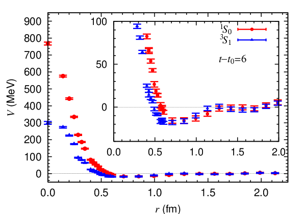
Figure 2 shows the (effective) central potentials for $p\Xi^{0}$ in the ${}^{1}S_{0}$ and ${}^{3}S_{1}$ channels. These results are still preliminary, since the potentials are obtained by assuming $E=0$: The energy should be determined by fitting the asymptotic behavior of the wave function with the use of the Green’s function $G(\vec{r},E)$ which is a solution of the Helmholtz equation on the lattice[12, 18]. Preliminary calculation suggests that $E$ would be small negative values for both ${}^{1}S_{0}$ and ${}^{3}S_{1}$ channels, similar to the case of the $NN$ potential[10, 19].

In order to see the ground state saturation of the present results, we plot, in Fig. 3, the time-slice dependence of the potential in both of the ${}^{1}S_{0}$ (left-hand-side) and ${}^{3}S_{1}$ (right-hand-side) channels at several radial distances; $r=0.14$, $0.20$, $0.71$, $1.42$, and $2.27$ fm. We can see that the saturation is achieved for $t-t_{0}\geq 6$ within errors.

The present work is a first step toward the $YN$ and $YY$ potentials from the lattice QCD simulation. Systematic studies of the various channels such as $\Lambda N$, $\Sigma N$, $\Lambda\Lambda$, and so on are all interesting and important because they are intimately related not only to the structure of hypernuclei but also to the internal structure of neutron stars. We will present such studies in the near future.