Let us switch to a new coordinate $y$ and to a new quantum parameter $\alpha$:

in terms of which the dependence of all the considered quantities on the charges is factorized³³ 3 For brevity’s sake, we write ${\tt Im\,}y^{n}$ instead of $({\tt Im\,}y)^{n}$. The same holds for ${\tt Re\,}y$.:

As stated above, the topology of the allowed regions of ${\tt Im\,}t$ depends on the sign of $\lambda$, as given by Fig. 1. In terms of $y$ and $\alpha$ defined in the BPS domain by Eq. (18), the corresponding allowed regions are represented in Fig. 2.

For example, if one considers $q_{0}<0$ then for $\alpha>0$ there are two disconnected allowed intervals for ${\tt Im\,}y$:

while for $\alpha<0$ it can range in only one interval:

In the classical case there is a one-to-one correspondence between the symplectic vector of BH charges inserted as input in the Attractor Eq. (8) and the solutions to this equation. Thus, for example in the BPS domain $p^{0}q_{1}>0$, when inserting two arbitrary values for $p^{0}$ and $q_{1}$ of the same sign, in the classical case there exists one and only one solution (in particular, of BPS type) to the classical Attractor Eq. (8).

This is no more true in the considered quantum case: in the BPS domain $p^{0}q_{1}>0$, when inserting two arbitrary values for $p^{0}$ and $q_{1}$ of the same sign, now there exist two stable critical points⁴⁴ 4 Also unstable non-BPS critical points of $V_{BH}$ may exist; however, we will not deal with them, because they do not determine attractors in strict sense. of $V_{BH}$, one BPS and the other non-BPS. It is worth remarking that in the considered BPS domain the non-BPS critical points of $V_{BH}$ do not admit a classical limit $\alpha\rightarrow 0$.

Furthermore, while in the classical case both BPS and non-BPS critical points of $V_{BH}$ supported by a “magnetic” BH charge configuration are axion-free, in the quantum case also non-BPS critical points of $V_{BH}$ with non-vanishing axion may arise out (and they can also be stable). As in the classical case, also in the considered quantum case non-BPS critical points of $V_{BH}$ with $Z=0$ do not exist at all. A pictorial view of the more complicated situation typical of the quantum case is given by Fig. 3. As mentioned in the Appendix, in both domains (BPS and non-BPS) of the quantum case the BPS solutions are known analytically, whereas the non-BPS solutions can be investigated only numerically.

Axion-free stable non-BPS critical points arise only for $\alpha>\frac{1}{3\sqrt{3}}$ (in the case $q_{0}<0$) and for $\alpha<-\frac{1}{3\sqrt{3}}$ (in the case $q_{0}>0$). On the other hand, non-BPS critical points with non-vanishing axion field exists only for $0<\alpha<\alpha_{cr_{1}}$ (in the case $q_{0}<0$) and for $-\alpha_{cr_{1}}<\alpha<0$ (in the case $q_{0}>0$), where the value of the $\alpha_{cr_{1}}$ is known just numerically: $\alpha_{cr_{1}}\in\left(0.030101,0.030102\right)$.

By looking at Fig. 3, one can realize at a glance that two new phenomena, absent in the classical case, arise in the quantum case. The first one, which we will name “separation” of attractors, occurs when the value of the quantum parameter is fixed in a certain range. The second one, which we will call “transmutation” of attractors, occurs when the value of the quantum parameter is varied, and becomes greater (or smaller) of a certain critical value.

Concerning the “separation”, from Fig. 3 one sees that for $|\alpha|<\alpha_{cr_{1}}$ two different stable critical points of $V_{BH}$ exist for the same BH charge configuration: one of them is BPS (whose classical limit is the well known BPS solution (9)), the other one is non-BPS with ${\tt Re\,}y\neq 0$ (which does not have a classical limit). Such a “separation” of the solutions of the Attractor Eq. (8) can ultimately be traced back to the presence of two disconnected regions in the domain of allowed values for ${\tt Im\,}y$ (see above treatment), which determines two disconnected regions of asymptotical ($r\rightarrow\infty$) values for ${\tt Im\,}y$ (also called “area codes” or “basins of attraction” in literature [62, 63, 64, 11, 39]). The dynamical radial evolution of the modulus $t$ is completely deterministic, and determines one unique solution for an arbitrary but fixed “magnetic” BH charge configuration given as input to the Attractor Eq. (8), but only inside each “area code”. Thus, the core of the Attractor Mechanism is preserved in the considered framework of dyonic, extremal, static, spherically symmetric and asymptotically flat BHs in $\mathcal{N}=2$, $d=4$ supergravity. In other words, the Attractor Mechanism gets two-fold split due to the presence of two disconnected regions in the allowed values of the modulus $t$, separated by a region where the metric function $g$ is negative. Such a result allows one to conjecturally argue that in presence of $m$ disconnected regions allowed in the moduli space, in general there exist $m$ solutions to the Attractor Eqs. for an arbitrary but fixed supporting BH charge configuration⁵⁵ 5 In the context of $n_{V}=1$ SK geometries, the phenomenon of “separation” of the solutions of the Attractor Eq. (8) can be observed also for more general geometries, which do not corrispond to cubic geometries in the large modulus limit. An example is given by the $1$-modulus SK geometry based on the holomorphic prepotential $\mathcal{F}=t^{4}$ (we thank Mario Trigiante for discussions on this issue).. A similar phenomenon was observed some years ago in $\mathcal{N}=2$, $d=5$ supergravity in [62, 63]; the disconnectedness of the moduli space preserves the validity of the Attractor Mechanism inside each allowed connected region, and therefore the results of existence and uniqueness of the solutions to the Attractor Eqs. obtained in [65] are still valid, but inside each “area code”.

Concerning the “transmutation”, let us take $q_{0}<0$ (this does not imply any loss of generality). Thence, from Fig. 3 one sees that varying the quantum parameter $\alpha$ across the critical value $\frac{1}{3\sqrt{3}}$ the BPS stable critical point “transmutes” into the non-BPS critical point (or vice versa).

By recalling that $\alpha$ depends on (a dimensionless ratio of) $q_{0}$ and $p^{1}$, it is easy to realize that the occurrence of such a phenomenon can be traced back to the fact that the supporting “magnetic” (branches of the) BH charge orbits still exist in the considered quantum case, but, as the quantum moduli space itself, they are not symmetric nor homogeneous manifolds any more.

As mentioned above, since the BPS critical points can be computed analytically, one can calculate the $\alpha$-dependent expression of the BPS BH entropy in the BPS domain to be

where the solution of the cubic Eq. must be chosen inside the allowed region(s) of the moduli space, and the $\pm$ branches of $S_{BH}$ must be chosen in order to obtain $S_{BH}>0$. In the classical limit $\alpha\rightarrow 0$, one recovers the well known value $S_{BH}=2\pi\sqrt{q^{0}(p_{1})^{3}}$ given by Eq. (10).

Let us now analyze the evolution $V_{BH}$ with respect to the quantum parameter $\alpha$. Choosing $q_{0}<0$ without loss of generality, we consider $\alpha>0$, because, due to the presence of the “separation” of attractors described above, it is the most interesting case.

The classical limit of the function $v$ defined in Eq. (19) has the form of a “scoop”, with a minimum at the point ${\tt Re\,}y=0$, ${\tt Im\,}y=1$ (see Eq. (9) and Fig. 4).

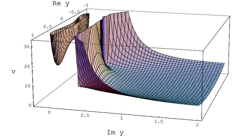
Let us now switch the (considered class of) quantum corrections on, and slightly increase the value of $\alpha$ from $0$ to $0.01$. As one can see from Fig. 3, $\alpha=0.01$ is in the range supporting the “separation” of attractors, i.e. the coexistence of the axion-free BPS attractors with the non-BPS ones with non-vanishing axion. Such stable critical points of $V_{BH}$ respectively have coordinates

As one can see from the plot of $V_{BH}$, in contrast to the classical case there appears a new chump of the form of camel humps, which contains a stable non-BPS critical point (not existing in the classical limit). The width of such a disconnected branch of $V_{BH}$ is $\sqrt[3]{\alpha/2}$, and thus it vanishes in the classical limit. The region of separation between the two branches of $V_{BH}$ has width $\sqrt[3]{\alpha}$, and in such a region $g<0$.

As yielded by Eq. (23), for $\alpha=0.01$ (and actually in the whole range of $\alpha$ supporting the “separation” of attractors) it holds that $V_{BH,BPS}<V_{BH,non-BPS}$. It is worth remarking that this is the opposite of what happens in globally supersymmetric field theories with multiple local minima, where the non-supersymmetric stable critical points of the superpotential are energetically favored with respect to their supersymmetry-preserving counterparts (see e.g. [66, 67, 68] and Refs. therein).

Increasing the value of $\alpha$ the flatness of the humps increases (on the figure 5 are presented sections of hump chump by planes ${\tt Re\,}y=const$ passing through minima),

and at the critical value $\alpha_{cr_{1}}$ the humps disappear. For $\alpha>\alpha_{cr_{1}}$ the non-BPS branch of $V_{BH}$ in the BPS domain does not contain critical points of $V_{BH}$ any more.

Let us now analyze the evolution of the BPS branch of $V_{BH}$ when increasing $\alpha$. When $\alpha\rightarrow\frac{1}{3\sqrt{3}}^{-}$, the BPS minimum point gets closer and closer to the boundary of the region where $g<0$ (see Fig. 2), until it sits exactly on the curve where the metric function vanishes, becoming a non-admissible critical point of $V_{BH}$ (red curve on the Fig. 5). Differently from what happens in the non-BPS branch when $\alpha$ gets bigger than $\alpha_{cr_{1}}$, in the BPS branch when $\alpha$ gets bigger than the critical value $\frac{1}{3\sqrt{3}}$ the critical point does not disappear, but rather it changes its supersymmetry-preserving features: from BPS it “transmutes” into a non-BPS one, preserving its axion-free character. Such a phenomenon of “transmutation” of attractors can be seen by looking at the  $q_{0}<0$ branch of Fig. 3: when $\alpha$ increases and it passes through $\frac{1}{3\sqrt{3}}$ the BPS minimum transforms into a non-BPS minimum.

Finally, it is worth plotting in Fig. 6 the $\alpha$-dependence of the BPS and non-BPS entropies (e.g. for $q_{0}<0$, without any loss of generality). Consistently with Fig. 3, the red line corresponds to BPS minima, the blue line to non-BPS minima with non-vanishing axion, and the green line to axion-free non-BPS minima. As it is seen, as previously mentioned in all the range of $\alpha$ supporting coexistence of minima it holds $S_{BH,BPS}<S_{BH,non-BPS}$.

Let us also notice that the definitions (18) are dimensionless in charges, and thus all considered phenomena hold for any magnitude of BH charges $q_{0}$ and $p^{1}$.

Let us switch to a new special coordinate $y$ and to a new quantum parameter $\alpha$ (notice the different definition with respect to the corresponding quantities in the BPS domain defined by Eq. (18)):

in terms of which the dependence of all the considered quantities on the charges is factorized:

Notice that $v(y,\bar{y},\alpha)$ defined in the non-BPS domain by Eq. (25) is different from its counterpart defined in the BPS domain by Eq. (19). As pointed out above, the topology of the allowed regions of ${\tt Im\,}t$ depends on the sign of $\lambda$, as given by Fig. 1. In terms of $y$ and $\alpha$ defined in the non-BPS domain by Eq. (24), the corresponding allowed regions are given by Fig. 7.

As in the BPS domain, also in the non-BPS domain the phenomena of “separation” and “transmutation” of attractors arise, but in a slightly different way. A pictorial view of the ranges of $\alpha$ supporting the various typologies of minima of $V_{BH}$ is given by Fig. 8. Differently from what happens in the BPS domain, in the non-BPS domain no non-BPS minima with non-vanishing axion exist at all, and there are two distinct typologies of axion-free non-BPS minima.

Concerning the BPS minima, for $q_{0}<0$ they exist in the range $0<\alpha<\frac{2}{3\sqrt{3}}$, whereas for $q_{0}>0$ they exist for $\alpha>\frac{2}{3\sqrt{3}}$. The same holds for $\alpha<0$, but with opposite sign of $q_{0}$.

As mentioned, in the considered non-BPS domain there are two kinds of non-BPS minima, both axion-free (see Fig. 8). The corresponding relevant critical value of the quantum parameter is $\alpha_{cr_{2}}\approx 0.934$.

As mentioned above, since the BPS critical points can be computed analytically, one can calculate the $\alpha$-dependent expression of the BPS BH entropy in the non-BPS domain to be

where the solution of the cubic equation must be chosen inside the allowed region(s) of the moduli space, and the $\pm$ branches of $S_{BH}$ must be chosen in order to obtain $S_{BH}>0$. As it has to be in the non-BPS domain, in the classical limit the cubic equation has no admissible solutions.

Let us now analyze the evolution $V_{BH}$ with respect to the quantum parameter $\alpha$, choosing $q_{0}<0$ without loss of generality.

The classical limit of the function $v$ defined in Eq. (25) has the form of a “scoop”, with a minimum at the point ${\tt Re\,}y=0$, ${\tt Im\,}y=1$ (see Eq. (9) and Fig. 9).

As done in the BPS domain, let us now slightly increase the value of $\alpha$ from $0$ to $0.01$. As one can see from Fig. 9, $\alpha=0.01$ is in the range supporting the “separation” of attractors, in this case corresponding to the coexistence of a BPS attractors with a non-BPS one, both axion-free. Such stable critical points of $V_{BH}$ respectively have coordinates

As one can see from the plot of $V_{BH}$ and analogously to what happens in the BPS domain, in contrast to the classical case there appears a new chump, which contains a stable BPS critical point (not existing in the classical limit). The width of such a disconnected branch of $V_{BH}$ (which vanishes in the classical limit) and its separation from the other branch admitting a consistent classical limit are both proportional to $\sqrt[3]{\alpha}$. As in the BPS domain, such two branches of $V_{BH}$ are separated by a region in which $g<0$.

As yielded by Eq. (27), for $\alpha=0.01$ it holds that $V_{BH,non-BPS}<V_{BH,BPS}$ (see discussion below).

However in the non-BPS domain, once again differently from the BPS domain, in the range $0<\alpha<\alpha_{cr_{2}}$ supporting the “separation” of attractors one can observe also the phenomenon of the “transmutation” of the supersymmetry-preserving features of the such minima of $V_{BH}$. This can be seen by increasing $\alpha$.

As evident by looking at Fig. 10, the scoop chump of $V_{BH}$ (i.e. the branch of $V_{BH}$ containing an axion-free non-BPS minimum and admitting a classical limit), does not undergo any qualitative change when increasing $\alpha$. On the other hand, the hump chump of $V_{BH}$ (i.e. the one vanishing for $\alpha\rightarrow 0$) exhibits a “transmutation” of the minimum: for $0<\alpha<\frac{2}{3\sqrt{3}}$ it constains a BPS minimum. For $\alpha=\frac{2}{3\sqrt{3}}$ such a critical point of $V_{BH}$ sits on the boundary (see Fig. 7) where $e^{K}$ diverges, so it is not an allowed critical point of $V_{BH}$. For $\frac{2}{3\sqrt{3}}<\alpha<\alpha_{cr_{2}}$ the minimum is still present, it is not BPS any more, but rather it is non-BPS (and axion-free). Thence, for $\alpha>\alpha_{cr_{2}}$ the hump chump of $V_{BH}$ does not contain any critical point.

Also the scoop chump of $V_{BH}$ exhibits a “transmutation” of the minimum, but for negative values of $\alpha$. Indeed, when $\alpha$ gets smaller than $-\frac{2}{3\sqrt{3}}$ the axion-free non-BPS minimum “transmutes” into a BPS one (axion-free, as all the admissible BPS critical points found in our analysis).

The shape of $V_{BH}$ for various values of $\alpha$ is plotted in Fig. 10. One might see that for small values of $\alpha$ (blue line) the hump chump contains a BPS minimum. At the critical value $\alpha=\frac{2}{3\sqrt{3}}$ (green line) the minimum disappears and reappears, but non-BPS, when $\alpha>\frac{2}{3\sqrt{3}}$ (red line). For $\alpha>\alpha_{cr_{2}}$, no critical points exist at all (black line).

The $\alpha$-dependence of the BH entropy is shown in Fig. 11. Consistently with the colors used in Fig. 8, the red plot corresponds to BPS BH entropy, whereas the blue and green plots to non-BPS BH entropy.

As done in the BPS domain, it is worth pointing out that the definitions (24) are dimensionless in charges, and thus all considered phenomena hold for any magnitude of BH charges $q_{0}$ and $p^{1}$.

Thus, the non-BPS domain exhibits various differences with respect to the BPS domain, which can be summarized as follows:

i) all non-BPS minima in such a domain are axion-free;

ii) the “transmutation” of the supersymmetry-preserving features of the minimum of $V_{BH}$ happens not only in the branch of $V_{BH}$ admitting a classical limit, but also in the one vanishing in such a limit;

iii) the “transmutation” inside the branch of $V_{BH}$ vanishing in the classical limit actually determines a “transmutation” in the region of “separation” of attractors: for $0<\alpha<\frac{2}{3\sqrt{3}}$ a BPS and a non-BPS minimum coexist; when $\alpha$ gets bigger than $\frac{2}{3\sqrt{3}}$ the BPS minimum “transmutes” into a non-BPS one, who then coexists with the pre-existing non-BPS (axion-free) minimum until $\alpha$ reaches the critical value $\alpha_{cr_{2}}$;

iv) as evident by looking at Fig. 11, in the range $0<\alpha<\frac{2}{3\sqrt{3}}$ supporting the coexistence of a BPS and a non-BPS minimum, the sign of $S_{BH,non-BPS}-S_{BH,BPS}$ (for fixed BH charges $p^{0}$ and $q_{1}$ satisfying $p^{0}q_{1}<0$) changes. Indeed, there exists a particular value $\widehat{\alpha}\approx 0.1\in\left(0,\frac{2}{3\sqrt{3}}\right)$ for which remarkably $S_{BH,non-BPS}=S_{BH,BPS}$. This means that for $\alpha=\widehat{\alpha}$ two different purely charge-dependent attractor configurations of the scalar $t$ exist (one preserving one half of the $8$ supersymmetries pertaining to the asymptotical $\mathcal{N}=2$, $d=4$ superPoincaré algebra and the other not preserving any of them) such that they determine the same BH entropy. For $0<\alpha<\widehat{\alpha}$ it holds $S_{BH,non-BPS}<S_{BH,BPS}$, whereas for $\widehat{\alpha}<\alpha<\frac{2}{3\sqrt{3}}$ it holds $S_{BH,BPS}<S_{BH,non-BPS}$;

v) for $\frac{2}{3\sqrt{3}}<\alpha<\alpha_{cr_{2}}$ it holds $\widetilde{S}_{BH,non-BPS}<S_{BH,non-BPS}$, where $\widetilde{S}_{BH,non-BPS}$ is the BH entropy determined by the non-BPS minimum originated from the BPS one by “transmutation” (see the green and blue plots in Fig. 11);

vi) for $\alpha>\alpha_{cr_{2}}$, the branch of $V_{BH}$ vanishing in the classical limit actually still contains critical points of $V_{BH}$, but they are not admissible and/or they are not stable.

It is worth pointing out that all the obtained results are expressed in terms of coordinates and quantum parameters dimensionless in the BH charges (i.e. depending on ratios of BH charges, as given by Eqs. (18) and (24)). Thus, apriori they hold for every range of values of the BH charges. Actually, we disregard the actual quantization of the electric and magnetic charges, considering $\mathbb{R}^{4}$, rather than the 4-dimensional charge lattice $\widehat{\Gamma}$, to be the space spanned by the BH charge vector $Q$. In other words, all our analysis and the obtained results hold in the semiclassical regime of large, continuous, real BH charges.

From the above analysis of the extremal BH attractors supported by the “magnetic” charge configuration $Q=\left(q_{0},0,0,p^{1}\right)$ in the $t^{3}+i\lambda$ model, one might be lead to argue that starting from a BH charge configuration supporting only one class of attractors at the classical level, at the quantum level one obtains that such a charge configuration generally supports more than one class of attractors (at least for a certain range of the quantum parameter $\lambda$).

This is actually not true, and a counterexample is provided by the BH charge configuration $Q=\left(q_{0},0,p^{0},0\right)$, usually named Kaluza-Klein BH (in $M$-theory language) [69] or $D0-D6$ system (in Type IIA Calabi-Yau compactifications in the language of superstring theory) [10, 34], for which the superpotential acquires the form

It is easy to check that at the classical level such a charge configuration only supports non-BPS attractors [10, 34, 40]. Differently from what happens for the “magnetic” charge configuration, this holds also at the quantum level, $\forall\lambda\in\mathbb{R}$; in other words, the $t^{3}+i\lambda$ model does not have admissible BPS critical points of $V_{BH}$ supported by the $D0-D6$ charge configuration. This can be easily realized by looking at the real and imaginary parts of the BPS Attractor Equation for such a charge configuration, respectively of the following form (having a smooth classical limit):

By recalling the expression of the metric function $g$ given by Eq. (12), it is clear that all BPS critical points of $V_{BH}$ supported by the $D0-D6$ charge configuration are points where $g=0$, and therefore they are not admissible.

Also in view of the analysis of [53], such a result can be directly extended to the axion-free BPS critical points of $V_{BH}$ in a $\mathit{\lambda}$-corrected SK cubic geometry, based on the Kähler gauge-invariant holomorphic prepotential (in a suitable basis of special symplectic coordinates $t^{i}\equiv\varsigma^{i}-i\omega^{i}$, $i=1,...,n_{V}$)

which is nothing but the $n_{V}$ moduli generalization of Eq. (11). The $\mathit{\lambda}$-corrected real metric $g_{ij}$ can be easily computed from Eq. (30) to be

where $d_{ij}\equiv d_{ijk}\omega^{k}$, $d_{i}\equiv d_{ijk}\omega^{j}\omega^{k}$ and $d\equiv d_{ijk}\omega^{i}\omega^{j}\omega^{k}$. Notice that the limit $\lambda\rightarrow 0$ consistently yields the expression of the real metric of a SK cubic geometry, given by Eq. (2.4) of [40]. In [53] the axion-free BPS critical points of $V_{BH}$ in the SK geometry based on $\mathcal{F}$ given by Eq. (30) have been computed to be

where the charge-dependent quantity $\mathfrak{c}$ satisfies the third order algebraic equation

It is then clear that the $D0-D6$ BH charge configuration does not support axion-free BPS critical points of $V_{BH}$, because for $p^{i}=0$ $\forall i=1,...,n_{V}$ Eqs. (31) and (32) yield $g_{ij,BPS,axion-free}=0$.

References

- [1] S. Ferrara, R. Kallosh and A. Strominger, Extremal Black Holes, Phys. Rev. D52, 5412 (1995), hep-th/9508072.
- [2] A. Strominger, Macroscopic Entropy of Extremal Black Holes, Phys. Lett. B383, 39 (1996), hep-th/9602111.
- [3] S. Ferrara and R. Kallosh, Supersymmetry and Attractors, Phys. Rev. D54, 1514 (1996), hep-th/9602136.
- [4] S. Ferrara and R. Kallosh, Universality of Supersymmetric Attractors, Phys. Rev. D54, 1525 (1996), hep-th/9603090.
- [5] S. Ferrara, G. W. Gibbons and R. Kallosh, Black Holes and Critical Points in Moduli Space, Nucl. Phys. B500, 75 (1997), hep-th/9702103.
- [6] A. Sen, Black Hole Entropy Function and the Attractor Mechanism in Higher Derivative Gravity, JHEP 09, 038 (2005), hep-th/0506177.
- [7] K. Goldstein, N. Iizuka, R. P. Jena and S. P. Trivedi, Non-Supersymmetric Attractors, Phys. Rev. D72, 124021 (2005), hep-th/0507096.
- [8] A. Sen, Entropy Function for Heterotic Black Holes, JHEP 03, 008 (2006), hep-th/0508042.
- [9] R. Kallosh, New Attractors, JHEP 0512, 022 (2005), hep-th/0510024.
- [10] P. K. Tripathy and S. P. Trivedi, Non-Supersymmetric Attractors in String Theory, JHEP 0603, 022 (2006), hep-th/0511117.
- [11] A. Giryavets, New Attractors and Area Codes, JHEP 0603, 020 (2006), hep-th/0511215.
- [12] K. Goldstein, R. P. Jena, G. Mandal and S. P. Trivedi, A C-Function for Non-Supersymmetric Attractors, JHEP 0602, 053 (2006), hep-th/0512138.
- [13] M. Alishahiha and H. Ebrahim, Non-supersymmetric attractors and entropy function, JHEP 0603, 003 (2006), hep-th/0601016.
- [14] R. Kallosh, N. Sivanandam and M. Soroush, The Non-BPS Black Hole Attractor Equation, JHEP 0603, 060 (2006), hep-th/0602005.
- [15] B. Chandrasekhar, S. Parvizi, A. Tavanfar and H. Yavartanoo, Non-supersymmetric attractors in gravities, JHEP 0608, 004 (2006), hep-th/0602022.
- [16] J. P. Hsu, A. Maloney and A. Tomasiello, Black Hole Attractors and Pure Spinors, JHEP 0609, 048 (2006), hep-th/0602142.
- [17] S. Bellucci, S. Ferrara and A. Marrani, On some properties of the Attractor Equations, Phys. Lett. B635, 172 (2006), hep-th/0602161.
- [18] S. Bellucci, S. Ferrara and A. Marrani, Supersymmetric Mechanics. Vol.2: The Attractor Mechanism and Space-Time Singularities (LNP 701, Springer-Verlag, Heidelberg, 2006).
- [19] S. Ferrara and R. Kallosh, On attractors, Phys. Rev. D 73, 125005 (2006), hep-th/0603247.
- [20] M. Alishahiha and H. Ebrahim, New attractor, Entropy Function and Black Hole Partition Function, JHEP 0611, 017 (2006), hep-th/0605279.
- [21] S. Bellucci, S. Ferrara, M. Günaydin and A. Marrani, Charge Orbits of Symmetric Special Geometries and Attractors, Int. J. Mod. Phys. A21, 5043 (2006), hep-th/0606209.
- [22] D. Astefanesei, K. Goldstein, R. P. Jena, A. Sen and S. P. Trivedi, Rotating Attractors, JHEP 0610, 058 (2006), hep-th/0606244.
- [23] R. Kallosh, N. Sivanandam and M. Soroush, Exact Attractive non-BPS STU Black Holes, Phys. Rev. D74, 065008 (2006), hep-th/0606263.
- [24] P. Kaura and A. Misra, On the Existence of Non-Supersymmetric Black Hole Attractors for Two-Parameter Calabi-Yau’s and Attractor Equations, Fortsch. Phys. 54, 1109 (2006), hep-th/0607132.
- [25] G. L. Cardoso, V. Grass, D. Lüst and J. Perz, Extremal non-BPS Black Holes and Entropy Extremization, JHEP 0609, 078 (2006), hep-th/0607202.
- [26] S. Bellucci, S. Ferrara, A. Marrani and A. Yeranyan, Mirror Fermat Calabi-Yau Threefolds and Landau-Ginzburg Black Hole Attractors, Riv. Nuovo Cim. 029, 1 (2006), hep-th/0608091.
- [27] G.L. Cardoso, B. de Wit and S. Mahapatra, Black hole entropy functions and attractor equations, JHEP 0703, 085 (2007) hep-th/0612225.
- [28] R. D’Auria, S. Ferrara and M. Trigiante, Critical points of the Black-Hole potential for homogeneous special geometries, JHEP 0703, 097 (2007), hep-th/0701090.
- [29] S. Bellucci, S. Ferrara and A. Marrani, Attractor Horizon Geometries of Extremal Black Holes, Contribution to the Proceedings of the XVII SIGRAV Conference,4–7 September 2006, Turin, Italy, hep-th/0702019.
- [30] A. Ceresole and G. Dall’Agata, Flow Equations for Non-BPS Extremal Black Holes, JHEP 0703, 110 (2007), hep-th/0702088.
- [31] L. Andrianopoli, R. D’Auria, S. Ferrara and M. Trigiante, Black Hole Attractors in Supergravity, JHEP 0707, 019 (2007), hep-th/0703178.
- [32] K. Saraikin and C. Vafa, Non-supersymmetric Black Holes and Topological Strings, hep-th/0703214.
- [33] S. Ferrara and A. Marrani, non-BPS Attractors, Fixed Scalars and Magic Supergravities, Nucl. Phys. B 2007, in press, ArXiV:0705.3866.
- [34] S. Nampuri, P. K. Tripathy and S. P. Trivedi, On The Stability of Non-Supersymmetric Attractors in String Theory, ArXiV:0705.4554.
- [35] L. Andrianopoli, R. D’Auria, E. Orazi, M. Trigiante, First Order Description of Black Holes in Moduli Space, ArXiV:0706.0712.
- [36] S. Ferrara and A. Marrani, On the Moduli Space of non-BPS Attractors for Symmetric Manifolds, Phys. Lett. B652, 111 (2007) , ArXiV:0706.1667.
- [37] D.Astefanesei and H. Yavartanoo, Stationary black holes and attractor mechanism, arXiv:0706.1847.
- [38] G. L. Cardoso, A. Ceresole, G. Dall’Agata, J. M. Oberreuter, J. Perz, First-order flow equations for extremal black holes in very special geometry, ArXiV:0706.3373.
- [39] A. Misra and P. Shukla, ’Area codes’, large volume (non-)perturbative alpha-prime and instanton: Corrected non-supersymmetric (A)dS minimum, the ’inverse problem’ and ’fake superpotentials’ for multiple-singular-loci-two-parameter Calabi-Yau’s, ArXiV:0707.0105.
- [40] A. Ceresole, S. Ferrara and A. Marrani, 4d/5d Correspondence for the Black Hole Potential and its Critical Points, Class. Quant. Grav. 2007, in press, ArXiV:0707.0964.
- [41] M. M. Anber and D. Kastor, The Attractor mechanism in Gauss-Bonnet gravity, arXiv:0707.1464.
- [42] Y. S. Myung, Y.-W. Kim and Y.-J. Park, New attractor mechanism for spherically symmetric extremal black holes, arXiv:0707.1933.
- [43] S. Bellucci, A. Marrani, E. Orazi and A. Shcherbakov, Attractors with Vanishing Central Charge, Phys. Lett. B 2007, in press, ArXiV:0707.2730.
- [44] K. Hotta and T. Kubota, Exact Solutions and the Attractor Mechanism in Non-BPS Black Holes, arXiv:0707.4554.
- [45] X. Gao, Non-supersymmetric Attractors in Born-Infeld Black Holes with a Cosmological Constant, arXiv:0708.1226.
- [46] S. Ferrara and A. Marrani, Black Hole Attractors in Extended Supergravity, to appear in the proceedings of 13th International Symposium on Particles, Strings and Cosmology (PASCOS 07), London, England, 2-7 Jul 2007, arXiv:0708.1268.
- [47] A. Sen, Black Hole Entropy Function, Attractors and Precision Counting of Microstates, arXiv:0708.1270.
- [48] A. Belhaj, L.B. Drissi, E.H. Saidi and A. Segui, Supersymmetric Black Attractors in Six and Seven Dimensions, arXiv:0709.0398.
- [49] L. Andrianopoli, S. Ferrara, A. Marrani and M. Trigiante, Non-BPS Attractors in d and d Extended Supergravity, arXiv:0709.3488.
- [50] A. Ceresole, R. D’Auria and S. Ferrara, The Symplectic Structure of Supergravity and Its Central Extension, Talk given at ICTP Trieste Conference on Physical and Mathematical Implications of Mirror Symmetry in String Theory, Trieste, Italy, 5-9 June 1995, Nucl. Phys. Proc. Suppl. 46 (1996), hep-th/9509160.
- [51] S. Cecotti, S. Ferrara and L. Girardello, Geometry of Type II Superstrings and the Moduli of Superconformal Field Theories, Int. J. Mod. Phys. A4, 2475 (1989).
- [52] R. D. Peccei and H. R. Quinn, Constraints imposed by CP conservation in the presence of instantons, Phys. Rev. D16, 1791 (1977) R. D. Peccei and H. R. Quinn, CP conservation in the presence of instantons, Phys. Rev. Lett. 38, 1440 (1977) R. D. Peccei and H. R. Quinn, Some aspects of instantons, Nuovo Cim. A41, 309 (1977).
- [53] K. Behrndt, G. Lopes Cardoso, B. de Wit, R. Kallosh, D. Lüst and T. Mohaupt, Classical and quantum supersymmetric black holes, Nucl. Phys. B488, 236 (1997), hep-th/9610105.
- [54] L. Alvarez-Gaume, D. Z. Freedman, Geometrical Structure and Ultraviolet Finiteness in the Supersymmetric Sigma Model, Commun. Math. Phys. 80, 443 (1981).
- [55] M. T. Grisaru, A. van de Ven and D. Zanon, Four Loop Beta Function for the and Supersymmetric Nonlinear Sigma Model in Two Dimensions, Phys. Lett. B173, 423 (1986) M. T. Grisaru, A. van de Ven and D. Zanon, Two Dimensional Supersymmetric Sigma Models on Ricci Flat Kähler Manifolds are not Finite, Nucl. Phys. B277, 388 (1986) M. T. Grisaru, A. van de Ven and D. Zanon, Four Loop Divergences for the Supersymmetric Nonlinear Sigma Model in Two Dimensions, Nucl. Phys. B277, 409 (1986).
- [56] P. Candelas, X. C. De La Ossa, P. S. Green and L. Parkes, A Pair of Calabi-Yau Manifolds as an Exactly Soluble Superconformal Theory, Nucl. Phys. B359, 21 (1991).
- [57] P. Candelas, X. C. De La Ossa, P. S. Green and L. Parkes, An Exactly Soluble Superconformal Theory from a Mirror Pair of Calabi-Yau Manifolds, Phys. Lett. B258, 118 (1991).
- [58] S. Hosono, A. Klemm, S. Theisen and Shing-Tung Yau, Mirror symmetry, mirror map and applications to Calabi-Yau hypersurfaces, Commun. Math. Phys. 167, 301 (1995), hep-th/9308122.
- [59] E. Witten, Dyons of charge e theta/2 pi, Phys. Lett. B86, 283 (1979).
- [60] S. Ferrara, J. A. Harvey, A. Strominger and C. Vafa, Second quantized mirror symmetry, Phys. Lett. B361, 59 (1995), hep-th/9505162 P. S. Aspinwall, An dual pair and a phase transition, Nucl. Phys. B460, 57 (1996), hep-th/9510142 D. R. Morrison and C. Vafa, Compactifications of F theory on Calabi-Yau threefolds. 1, Nucl. Phys. B473, 74 (1996), hep-th/9602114 D. R. Morrison and C. Vafa, Compactifications of F theory on Calabi-Yau threefolds. 2, Nucl. Phys. B476, 437 (1996), hep-th/9603161 J. A. Harvey and G. W. Moore, Exact gravitational threshold correction in the FHSV model, Phys. Rev. D57, 2329 (1998), hep-th/9611176 A. Klemm and M. Marino, Counting BPS states on the Enriques Calabi-Yau, hep-th/0512227 J. R. David, On the dyon partition function in theories, arXiv:0711.1971.
- [61] M. Shmakova, Calabi-Yau black holes, Phys. Rev. D56, 540 (1997), hep-th/9612076.
- [62] A. Chou, R. Kallosh, J. Rahmfeld, Soo-Jong Rey, M. Shmakova and Wing Kai Wong, Critical points and phase transitions in 5-d compactifications of M-theory, Nucl. Phys. B508, 147 (1997), hep-th/9704142.
- [63] R. Kallosh, A. D. Linde and M. Shmakova, Supersymmetric multiple basin attractors, JHEP 9911, 010 (1999), hep-th/9910021.
- [64] G.W. Moore, Attractors and Arithmetic, hep-th/9807056 G.W. Moore, Arithmetic and Attractors, hep-th/9807087 G.W. Moore, Les Houches Lectures on Strings and Arithmetic, hep-th/0401049.
- [65] M. Wijnholt and S. Zhukov, On the Uniqueness of Black Hole Attractors, hep-th/9912002.
- [66] K. Intriligator and N. Seiberg, Lectures on Supersymmetry Breaking, hep-ph/0702069.
- [67] H. Ooguri and C. Vafa, On the Geometry of the String Landscape and the Swampland, Nucl. Phys. B766, 21 (2007), hep-ph/0605264.
- [68] H. Ooguri, The Entropic Principle, lectures given at the International School of Subnuclear Physics, 45th Course : Searching for the “Totally Unexpected” in the LHC Era, EMFCSC, 29 Aug. - 7 Sept. 2007, Erice, Italy, to appear in the Proceedings.
- [69] S. Ferrara and J. M. Maldacena, Branes, central charges and -duality invariant BPS conditions, Class. Quant. Grav. 15, 749 (1998), hep-th/9706097.