Memory effects in quantum information transmission across a Hamiltonian dephasing channel

Quantum information is the information related to a quantum source Schumacher95; BarnumNielsenSchumacher98, that is, a source $\Sigma$ of identical quantum systems $\cal Q$, which are prepared in an unknown quantum state chosen from the ensemble $\{\rho_{k}\}$, according to a given stationary probability distribution $\{p_{k}\}$. The amount of information generated by the source is measured by the von Neumann entropy $S(\Sigma)\equiv S(\rho)=-\mathrm{Tr}\big[\rho\log_{2}\rho\big]$, where $\rho=\sum_{k}p_{k}\rho_{k}$ Schumacher95; BarnumNielsenSchumacher98. Indeed, $S(\Sigma)$ provides the number of quantum two level systems necessary to efficiently encode the source $\Sigma$ according to the noiseless quantum coding theorem. Quantum information reduces to classical information only if the states $\{\rho_{k}\}$ are pure and mutually orthogonal.

A proper way to measure reliability of quantum information transmission is the entanglement fidelity Schumacher96; BarnumKnillNielsen00. To define this quantity we look at the system ${\cal Q}$ as a part of a larger quantum system ${\cal RQ}$, initially in a pure entangled state $|\psi^{\cal RQ}\rangle$. The density operator of the system ${\cal Q}$ is then obtained from that of ${\cal RQ}$ by a partial trace over ${\cal R}$: $\rho^{\cal Q}=\mathrm{Tr}_{\cal R}[|\psi^{\cal RQ}\rangle\langle\psi^{\cal RQ}|]$. The system ${\cal Q}$ is sent through the channel and undergoes the transformation ${\cal E}$, while ${\cal R}$ is ideally isolated from the environment (see Fig. (1) left). The final state of the composite system is:

where ${\cal I}$ is the identity superoperator.

Let us consider the following question: how faithfully does the channel preserve the entanglement between the two systems $\cal Q$ and $\cal R$? The answer is the entanglement fidelity $F_{e}$ Schumacher96, defined as the fidelity $F$ between the initial pure state $|\psi^{\cal RQ}\rangle$ and the final (generally mixed) state $\rho^{{\cal RQ}^{\prime}}$:

It can be shown that entanglement fidelity only depends on the initial state $\rho^{\cal Q}$ of the system and on the channel action ${\cal E}$, not on the particular purification $|\psi^{\cal RQ}\rangle$ chosen Schumacher96. Unlike the usual input-output fidelity kn:nielsen-chuang; kn:benenti-casati-strini, entanglement fidelity looks at the same physical process, the transmission of $\cal Q$ across a channel, from a different point of view: as a local transformation on a part ($\cal Q$) of an entangled system ($\cal RQ$). This transformation is undesired because it can reduce the amount of entanglement of the overall system.

The entropy exchange Schumacher96 is the entropy that the enlarged system ${\cal RQ}$ acquires when $\cal Q$ undergoes the transformation ${\cal E}$:

where $\rho^{{\cal RQ}^{\prime}}$ is given by (1). It can be shown that the entropy exchange is an intrinsic function of the system input $\rho^{\cal Q}$ and of the channel $\cal E$ and does not depend on the particular purificationSchumacher96. Since $\cal E$ is a completely positive trace preserving linear map, it can be represented kn:nielsen-chuang; kn:benenti-casati-strini by a unitary evolution $U^{{\cal Q}E}$ on a larger system, given by the system $\cal Q$ itself plus an ancilla $E$, that is, a (generally fictitious) environment initially in a pure state (see Fig. (1) right). It is straightforward to show that Schumacher96; SchumacherNielsen96:

where $\rho^{E^{\prime}}$ is the final state of the environment. $S_{e}$ measures the entropy increase of the environment $E$ or, equivalently, the entanglement between $\cal RQ$ and $E$ after the evolution $U$. The entropy exchange can be thought of as the quantum analogue of the classical conditional entropy Shannon48; CoverThomas91, that measures the average uncertainty about the channel output for a known input, namely the noise added to the output by the channel.

Classical channel capacity is given by the maximum (over the input probability distribution) of the input-output mutual information Shannon48; CoverThomas91. The quantity analogous to mutual information for quantum information is the coherent information $I_{c}$ SchumacherNielsen96; Lloyd97, defined as

For memoryless channels and for the so-called forgetful channels KretschmannWerner05, for which memory effects decay exponentially with time, the quantum channel capacity $Q$ is the maximum of $I_{c}/N$ over all possible input states, in the limit of number of channel uses $N\to\infty$ barnum; shor; devetak; winter. Note that the coherent information is maximal when ${\cal Q}$ and ${\cal R}$ are maximally entangled and the channel is noiseless. Indeed, in this case $S\big(\rho^{\cal Q^{\prime}}\big)=S\big(\rho^{\cal Q}\big)$ is maximal because the input state $\rho^{\cal Q}$ is maximally mixed, and $S\big(\rho^{{\cal RQ}^{\prime}}\big)=0$, since the state $|\psi^{\cal RQ}\rangle$ remains pure after the transmission. Smaller values of the coherent information are obtained when the state $|\psi^{\cal RQ}\rangle$ is not maximally entangled or noise affects the channel. This example illustrates the fact that coherent information measures the possibility to convey entanglement through a communication channel.

We consider the transmission of two qubits, ${\cal Q}_{1}$ and ${\cal Q}_{2}$, initially in the state $\rho^{{\cal Q}_{1}{\cal Q}_{2}}$, with matrix elements $\rho_{mn}$, $m,n=0,...,3$. The final state of the system is

where the factors $g$ and $h^{\pm}$ describe the channel effects and the noiseless limit is recovered for $g=h^{\pm}=1$. The last two terms are defined as

and are derived from (12) for $j_{1}=j_{2}=j$, $l_{1}=l_{2}\neq j$ ($h^{+}$) and for $j_{1}=l_{2}=j$, $j_{2}=l_{1}\neq j$ ($h^{-}$).

In the absence of any memory effects, that is, when the power spectrum $S(\omega)$ is white and there is no superposition between the time windows when the first or the second qubits are inside the channel ($\tau\geq\tau_{p}$), we have $h^{\pm}=g^{2}$; therefore, ${\cal E}_{2}={\cal E}_{1}\otimes{\cal E}_{1}$. In the opposite limiting case of perfect memory, that is, when $\tau_{c}\gg\tau,\tau_{p}$, or alternatively the two time windows of the qubit-environment interaction are completely superimposed ($\tau=0$), we have $h^{+}=g^{4}$ and $h^{-}=1$. In this limit the subspace spanned by the basis $\{|00\rangle\,,|11\rangle\}$ undergoes a stronger decoherence (with respect to the memoryless case), while the subspace spanned by $\{|01\rangle\,,|10\rangle\}$ is decoherence free.

It is convenient to measure the memory between two channel uses by introducing the memory coefficient $\gamma$ defined as follows:

For a given power spectrum $S(\omega)$ and crossing time $\tau_{p}$, $\gamma$ only depends on the time interval $\tau$, and ranges in the interval $[0,1]$. In particular, $\gamma=0$ for a memoryless channel (as it can be checked by letting $\tau\to\infty$ in the (27)), while $\gamma=1$ for perfect memory ($\tau=0$ in (27)). We can express the dephasing factors $h^{\pm}$ by means of the corresponding memoryless value $g^{2}$ and the memory factor $\gamma$:

In presence of memory ($\gamma>0$), the Kraus representation in our Hamiltonian model cannot be trivially derived from (15) by simply concatenating the Kraus operators for single channel use with a suitable probability distribution:

where the $B_{m}$ operators are the same as in (15). It is worth noting that in (29) memory could be taken into account by means of the joint probability $p(m_{2},m_{1})=p(m_{2}|m_{1})p(m_{1})$, where the conditional probability $p(m_{2}|m_{1})$ can introduce a correlation between the occurrence of the second qubit operator $B_{m_{2}}$ and the action of first qubit operator $B_{m_{1}}$. For simplicity we rename all possible combinations of the $B_{m}$ operators in (29): $K_{0}\equiv B_{0}\otimes B_{0}$, $K_{1}\equiv B_{0}\otimes B_{z}$, $K_{2}\equiv B_{z}\otimes B_{0}$ and $K_{3}\equiv B_{z}\otimes B_{z}$. It turns out that the Kraus representation for the map eq. (5.1) requires two other operators $K_{4}\equiv\frac{1}{2}(K_{1}+K_{2})$ and $K_{5}\equiv\frac{1}{2}(K_{0}-K_{3})$:

where $p_{K_{0}}=\frac{1}{4}(1+2g+h^{+})$, $p_{K_{1}}=p_{K_{2}}=\frac{1}{4}(1-h^{-})$, $p_{K_{3}}=\frac{1}{4}(1-2g+h^{+})$ and $p_{K_{4}}=p_{K_{5}}=\frac{1}{4}(h^{-}-h^{+})$. For $\gamma=0$, (30) is exactly equivalent to concatenating twice (15), namely ${\cal E}_{2}={\cal E}_{1}\otimes{\cal E}_{1}$. The behaviour of the (29) and (30) are very different. In fact for perfect memory the first Kraus representation, in which we have to set $p(m_{2}|m_{1})=\delta_{m_{2},m_{1}}$, generates two decoherence free subspaces: $\{|00\rangle\,,|11\rangle\}$ as well as $\{|01\rangle\,,|10\rangle\}$.

The purpose of this section is to show that memory effects can improve the channel performance. We consider diagonal input states of the type

This density operator describes a mixture in which we have, with probability $p$, the unpolarized state of the subspace spanned by $\{|01\rangle\,,|10\rangle\}$ and, with probability $q=1-p$, the unpolarized state of the subspace spanned by $\{|00\rangle\,,|11\rangle\}$. One can tune $p$ to increase the weight of the first subspace which - in the presence of memory - is protected against noise. On the other hand, the amount of input information, measured by the von Neumann entropy $S\big(\rho^{{\cal Q}_{1}{\cal Q}_{2}}\big)$, is maximal when $p=q$. We can purify system ${\cal Q}_{1}{\cal Q}_{2}$ by means of a two-qubit reference system ${\cal R}_{1}{\cal R}_{2}$. We choose, for the system ${\cal R}_{1}{\cal R}_{2}{\cal Q}_{1}{\cal Q}_{2}$, the following pure state:

After the qubits ${\cal Q}_{1}$ and ${\cal Q}_{2}$ have crossed the channel, the system ${\cal R}_{1}{\cal R}_{2}{\cal Q}_{1}{\cal Q}_{2}$ is described by the density operator

where the dots stand for zeros (the matrix has dimension $2^{4}\times 2^{4}$).

The entanglement fidelity is

and after some calculations we obtain

In Fig 2, we show several plots of the two-qubit entanglement fidelity (36). We can say that memory effects always improve this quantity, provided that the factor $p$ is properly chosen. This effect is more evident for strong dephasing (see Fig. 2(c)).

We now turn our attention to the entropy exchange

where the non-trivially equal to zero eigenvalues $\lambda_{m}$ of the output density operator (5.3) are given by

with

As shown in Fig. 3, memory effects lower the entropy exchange, that is, memory reduces to some extent the information on the system acquired by the channel-environment. These plots are complementary to those in Fig. 2: as expected from the quantum Fano inequality Schumacher96, the information exchanged with the environment is small when the disturbance of the state is small, namely $S_{e}$ is close to zero when $F_{e}$ is close to one. The numerical data of Figs. 2-3 also show that $S_{e}$ is close to one when $F_{e}$ is close to zero.

Finally we turn to the coherent information

Since the coherence terms in $\rho^{{\cal Q}_{1}{\cal Q}_{2}}$ are equal to zero, the dephasing channel does not change this state and therefore $S(\rho^{{\cal Q}_{1}^{\prime}{\cal Q}_{2}^{\prime}})=S(\rho^{{\cal Q}_{1}{\cal Q}_{2}})=-p\log_{2}\frac{p}{2}-q\log_{2}\frac{q}{2}$ and

We can see from fig. 4 that coherent information is highly sensitive to memory effects. This sensitivity depends on the dephasing factor $g$. When dephasing is strong ($g$ close to zero), strong memory effects are required to enhance the coherent information (see Fig. 4(c)), while for weaker dephasing (panels (a) and (b) in the same figure) it is possible to tune $p$ to obtain noticeable enhancements also with weak memory effects. It is interesting to examine the limiting case of perfect memory ($\gamma=1$) and to find, as a function of $g$, the value $p_{\rm opt}$ that maximizes the coherent information achievable for input state as in (31). Fig 5 shows that also in the regime of strong dephasing ($g<0.5$) reliable transmission can be obtained, provided we exploit the decoherence-protected subspace $\{|01\rangle\,,|10\rangle\}$, that is, $p_{\rm opt}$ is close to one.

We show that memory effects can be used to preserve entanglement in quantum information transmission. In particular, we consider an entanglement sharing protocol: Alice wish to send one qubit of a Bell pair (qubits ${\cal R}$ and ${\cal Q}$) to Bob. The quantum channel (6),(11) randomizes the phase between the sent qubit (${\cal Q}$) and the reference one (${\cal R}$). In order to take advantage of memory effects, we follow the strategy sketched in Fig 6. We encode the sent qubit in a two-qubit system whose state resides in the subspace (spanned by $\{|01\rangle\,,|10\rangle\}$) resilient to errors in the presence of memory effects.

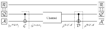
Without loss of generality we assume that the initial Bell state of the entangled pair is $|\psi^{\cal RQ}\rangle\,=\frac{1}{2}\big(|00\rangle+|11\rangle\big)=|\phi^{+}\rangle$. The coding-decoding protocol is performed in the following way:
(a) We prepare an ancillary qubit $\cal A$ in the state $|1\rangle^{\cal A}$, such that the whole system ${\cal RQA}$ is initially in the state

(b) The encoding operation $\cal C$ is a controlled-not gate acting on the system $\cal QA$, where $\cal Q$ is the control qubit:

As a result, we encode the system $\cal RQA$ into a GHZ state, in such a way that the subsystem ${\cal Q}{\cal A}$ resides in the subspace spanned by $\{|01\rangle\,,|10\rangle\}$. This is the case when the entangled state $|\psi^{\cal R\cal Q}\rangle$ is any state of the Bell basis:

(c) We send qubits ${\cal Q}$ and ${\cal A}$ through the channel. We call $\tilde{\rho}^{\cal RQ^{\prime}A^{\prime}}$ the density operator describing the state that arises from the channel transmission:

(d) The decoding operation $\cal D$ extracts the state of system ${\cal RQ}$ from the one of $\cal RQA$. To this aim we apply another controlled-not gate to the system $\cal QA$, where $\cal Q$ is - as above - the control qubit. This operation disentangles systems $\cal RQ$ and $\cal A$:

where

The fidelity of the final state $\rho^{\cal RQ^{\prime}}$ is

This is also the entanglement fidelity $F_{e}^{c}$ when the initial state of $\cal Q$ is $\rho^{\cal Q}=\frac{1}{2}{\hbox{\small 1\kern-3.8pt\normalsize 1}}$ and when the above coding-encoding scheme is used. We compare this value with the entanglement fidelity (17), obtained when the qubit ${\cal Q}$ is simply sent down the channel. Therefore, the above coding-encoding strategy is useful when memory effects are strong enough, namely when

In spite of its simplicity, coding/deconding schemes similar to the one described in this section can be useful to protect information in the presence of memory effects Yamamoto.