grand unification on a domain-wall brane from an -invariant action
Abstract
An grand unification scheme for effective -dimensional fields dynamically localised on a domain-wall brane is constructed. This is achieved through the confluence of the clash-of-symmetries mechanism for symmetry breaking through domain-wall formation, and the Dvali-Shifman gauge-boson localisation idea. It requires an gauge-invariant action, yielding a domain-wall solution that has broken to differently embedded subgroups in the two bulk regions on opposite sides of the wall. On the wall itself, the unbroken symmetry is the intersection of the two bulk subgroups, and contains . A -dimensional fermion family in the of gives rise to localised left-handed zero-modes in the representation of . The remaining ten fermion components of the are delocalised exotic states, not appearing in the effective -dimensional theory on the domain-wall brane. The scheme is compatible with the type-2 Randall-Sundrum mechanism for graviton localisation; the single extra dimension is infinite.
I Introduction
If our universe is a -dimensional brane Rubakov and Shaposhnikov 1983; Akama 1983; Visser 1985; Gibbons and Wiltshire 1987; Arkani-Hamed et al. 1998; Antoniadis 1990; Antoniadis et al. 1998; Randall and Sundrum 1999a; Randall and Sundrum 1999b existing in a -dimensional spacetime, then the most likely field-theoretic origin for the brane is a scalar-field domain wall (DW) or kink Rubakov and Shaposhnikov 1983. This generic idea is naturally compatible with the type-2 Randall-Sundrum (RS2) mechanism for producing effective -d gravity on the brane Randall and Sundrum 1999b (see, for example, Refs. Gremm 2000; DeWolfe et al. 2000; Davidson and Mannheim 2000 for the extension of thin-brane RS2 to a domain-wall brane). The challenge is to dynamically localise all the other ingredients necessary for a phenomenologically successful effective theory on the brane: gauge bosons, fermions, and Higgs bosons. Various localisation ideas for these disparate classes of fields have been recently combined to produce an effective brane theory that is plausibly very similar to the standard model Davies et al. 2007.
The purpose of this paper is twofold. First, we wish to point out a very elegant generic connection between the clash-of-symmetries (CoS) mechanism for symmetry breaking through domain wall formation Davidson et al. 2002; Rozowsky et al. 2004; Dando et al. 2005; Shin and Volkas 200411 1 See also Pogosian and Vachaspati 2000; Vachaspati 2001; Pogosian and Vachaspati 2001 for related works, and Dvali and Shifman 1997a for soliton-induced supersymmetry breaking., and the Dvali-Shifman (DS) idea for dynamical gauge-boson localisation Dvali and Shifman 1997b. Second, we use this remarkable confluence to construct an explicit scheme that realises an gauge-invariant effective theory on the brane. In a sense, it is a grand unified extension of the model of Ref. Davies et al. 2007, but the way in which the Dvali-Shifman mechanism is realised is quite different, and we shall argue that it is in fact conceptually more advanced. Remarkably, this scheme immediately produces a realistic spectrum of localised fermion zero-modes Jackiw and Rebbi 1976 (for a review see Rubakov 2001) using the simplest possible mechanism. While it is beyond the scope of this paper to write down a complete phenomenologically-acceptable domain-wall-brane localised theory, we shall conclude with brief remarks about how this could be attempted.
The clash-of-symmetries phenomenon Davidson et al. 2002; Rozowsky et al. 2004; Dando et al. 2005; Shin and Volkas 2004; Pogosian and Vachaspati 2000; Vachaspati 2001; Pogosian and Vachaspati 2001 automatically arises when the simple kink is extended to a theory with a continuous internal symmetry group in addition to the discrete symmetry. Taking the scalar-field multiplet to be in a non-trivial representation of , the domain-wall configuration spontaneously breaks in addition to reflecting the disconnected vacuum manifold topology created by the spontaneous breaking of the discrete symmetry. Two classes of domain-wall solutions exist: those which respect the same subgroup of at all values of the bulk coordinate , and those where the unbroken subgroup varies in the bulk. We shall call the first class “non-CoS domain walls”, contrasted with the “CoS domain walls” of the second class. Clash-of-symmetries DWs can arise when the subgroups respected asymptotically (at ) are isomorphic but differently embedded subgroups, and . The symmetry group at finite is typically the intersection , which is of course smaller than both and .
The last observation provides an immediate connection with the Dvali-Shifman proposal for dynamical gauge-boson localisation. The DS mechanism, as originally proposed Dvali and Shifman 1997b, envisaged a domain wall configuration where the full group is restored in the bulk, but broken to in the wall. The gauge bosons of propagate on the wall either as massless Abelian gauge fields or glueballs formed from non-Abelian gauge fields. In the bulk, all gauge bosons have to be incorporated into massive -glueballs.22 2 The Dvali-Shifman mechanism requires a confining -dimensional gauge theory to live in the bulk. The issue of confinement in dimensions is not completely understood, so the Dvali-Shifman mechanism in that context has the status of being a plausible conjecture. There is good lattice gauge theory evidence that pure Yang-Mills theory with an ultraviolet cut-off is confining in dimensions when the gauge coupling constant exceeds a certain critical value Creutz 1979. It is thus plausible that a variety of dimensional gauge theories exhibit confinement at sufficiently large coupling strength. Thus, the massless Abelian gauge fields on the wall have to become incorporated into massive glueballs in the bulk, and the energy cost associated with the mass gap then plausibly localises them to the wall. This heuristic argument is bolstered by the dual-superconductivity model ’t Hooft 1976; Mandelstam 1976 for the confining bulk: the electric field lines from a source charge in the wall are repelled from the interface with the dual-superconducting bulk Arkani-Hamed and Schmaltz 1999; Dubovsky and Rubakov 2001, just as magnetic field lines are Meissner-repelled from an ordinary superconductor. The non-Abelian gauge fields of are also plausibly localised if the mass of the -glueballs exceeds the mass of the -glueballs.
The fact that the full symmetry is asymptotically restored is clearly not a necessary condition. In the CoS situation, the brane-group is a subgroup of both and , the unbroken symmetries in the two semi-infinite bulk regions. By the DS reasoning, provided and contain confining non-Abelian factors, at least some of the gauge bosons of will be localised. For a realistic theory, we need the localised gauge bosons to include those of the standard model. The model-builder needs to engineer the theory to achieve this effect. While this engineering shall be the main concern in the rest of the paper, our first generic point has already been made: the clash-of-symmetries automatically gives rise to Dvali-Shifman gauge-boson localisation. This CoS alternative realisation of the DS mechanism seems conceptually neater than the original, because it can be achieved using scalars in a single irreducible representation of . The original requires two multiplets: a -singlet to form a kink, which in turn forces a -multiplet to condense in the core of the wall.
We shall show that the CoS-DS confluence can naturally produce an effective theory on the brane. The basic ingredients are , with the DW-producing scalar field in the adjoint or representation. The groups and will be the differently-embedded maximal subgroups and , respectively. Their intersection is , with of course being a subgroup of both and . Taking both of those as confining gauge theories in the bulk, the localisation of gauge bosons follows from the DS-effect. The gauge fields of are not completely localised. When -d fermions in the of are Yukawa-coupled to the scalar multiplet, we shall show that -d left-chiral zero-modes in the phenomenologically-realistic representation of are localised. The remaining ten fermion components remain -d, and are thus absent from the effective brane-theory. The result that the chiralities of the zero-modes come out to be phenomenologically correct is very non-trivial, as we shall explain.
II The clash of symmetries
Consider a theory (an action) whose symmetry group is the direct product of a continuous symmetry group and a discrete symmetry . It is important that is not a subgroup of . Suppose the global minima of the Higgs potential spontaneously break to subgroup , and simultaneously break to a smaller discrete group. For the sake of definiteness, we shall take the example in what follows, with the completely broken.
The vacuum manifold then consists of two disconnected copies of the coset space , with the copies related by the spontaneously broken . This is an immediate generalisation of the simple kink situation, where the vacuum manifold consists of just two disconnected points related by . Each such point is expanded into the non-trivial manifold . We shall call the disconnected pieces and . The must not be a subgroup of for the two disconnected pieces to exist.
Let be an element of . By definition, for all . Since the Higgs potential is -invariant, if we apply a transformation (that is, a transformation such that but ) to , we obtain a degenerate vacuum state . By considering all possible ’s, these transformations generate the piece of the vacuum manifold. Applying the non-identity transformation from the discrete group, we obtain the discrete image of . This image is a point in the other disconnected piece of the full vacuum manifold. By applying all possible to , the space is generated. Figure 1 illustrates this situation.
The degenerate vacua and respect differently embedded but otherwise isomorphic subgroups and , respectively. This is elementary: Let such that . Then the conjugates respect the same multiplication table and hence the set is precisely which is isomorphic to but a different subset of . If , then trivially , which simply says that the conjugated elements preserve the other vacuum: . Similar statements are true for .

The boundary conditions at for domain wall configurations are chosen from the vacua. If the chosen vacua are either both from , or both from , then the “domain wall” configurations are not topologically stable: they are in the same topological class as any of the spatially-homogeneous vacua , or respectively , and will dynamically decay to one of these vacua. They may be metastable, depending on the Higgs potential topography,33 3 We dread to use the term “landscape”. so while they are of some interest we shall not consider them further in this paper.
Topologically non-trivial DW configurations have one boundary condition from and the other from . Evidently, there is an uncountable infinity of such choices, and thus potentially an uncountable infinity of DW solutions, all within the same non-trivial topological class. Figure 1 illustrates the plethora of choices. This potential richness has no analogue for the simple kink.
Suppose that the boundary condition at is and at it is . Then if , it also follows that
| (1) |
because by assumption the symmetry is so that and hence always. Thus, the unbroken symmetry at is precisely the same set as at . A domain wall configuration that interpolates between these vacua is then expected to respect the same subgroup at all . This is an example of a non-CoS domain wall. Clearly, taking the vacua as any pair and produces a similar outcome (the resulting configuration is nothing more than the transform of the original one). A non-CoS domain wall is the simplest possible generalisation of a kink for a -invariant theory.
However, there is obviously a second, more interesting possibility: if the vacuum is at , then the vacuum at can also be a for . In that case, the subgroups respected asymptotically are the differently-embedded but isomorphic groups and , respectively. This defines a CoS-style domain wall Davidson et al. 2002; Rozowsky et al. 2004; Dando et al. 2005; Shin and Volkas 2004; Pogosian and Vachaspati 2000; Vachaspati 2001; Pogosian and Vachaspati 2001. At finite , the configuration would be expected to respect the smaller group due to the fact that the solution has to ‘‘reconcile’’ boundary conditions that have different stability groups that ‘‘clash’’.44 4 From experience, we have found that is the usual outcome. The specifics depend on the case considered. Sometimes there is enhanced symmetry at because some of the scalar multiplet components instantaneously vanish there. This enhancement on a set of measure zero has yet to find application, although speculations exist Shin and Volkas 2004; Demaria and Volkas 2005.
So, there will be an infinite family of non-CoS DWs, trivially related to each other by global transformations . They all have the same energy density, because the Hamiltonian is invariant under . The CoS DWs have a more complicated spectrum. Consider two configurations, and , with interpolating between and , while interpolates between and , such that . Suppose, for the moment, that is a global but not a local symmetry. These two solutions cannot be transformed into each by a global -transformation, so they would be expected to have different energy densities (their configurations trace different paths through the Higgs potential topography). As a corollary, the non-CoS solutions should have a different energy density from the CoS solutions. All these solutions are in the same topological class, so finite-energy dynamical evolution between them is allowed. Hence, the special configurations within that topological class that minimise the energy density will be topologically stable. The others should be unstable to decay to the minimum-energy configurations, which play the role of “vacua” for the “kink-sector”. This general reasoning cannot tell you which configuration has the minimum energy-density: you need to calculate that within a specific model. For example, in the toy model considered in Ref. Davidson et al. 2002 the sign of a Higgs potential parameter determined whether the non-CoS or a CoS solution was energetically favoured.
Suppose now that is a gauge symmetry, and again consider the configurations discussed in the previous paragraph, together with the specification of vanishing gauge fields at the solution-level. The non-CoS solutions remain connected through global transformations. Two CoS scalar field configurations, and , can be written as local -transforms of each other. Suppose that
| (2) |
where is a local- element. Then the original first solution
| (3) |
is gauge-equivalent to
| (4) |
where is the gauge coupling constant, but it is not gauge-equivalent to
| (5) |
which is the original second solution. Thus the two solutions and have different energy densities, even though the scalar-field portions are related by a local symmetry transformation. Although is a pure-gauge configuration, it contributes to the energy density through the interaction terms.
Setting the gauge fields to zero at the solution-level is basically a convenient choice of gauge, one we shall adopt from now on. Of course the solutions can be made to look very different by gauge-transforming them, but their physical consequences cannot change. This circumstance is no different from the monopole or local-string cases, where again the solutions look different in different gauges. Actually, it is no more complicated than the usual homogeneous vacuum expectation value (VEV) case. If is a homogeneous VEV, then it can be gauge-transformed to a non-homogeneous configuration but the scalar gradient energy is cancelled by the gauge-field contribution.
The alert reader may have noticed the following: we have not proven that the minimum-energy DW configuration must have a gauge-field sector that is gauge-equivalent to zero. This does indeed appear to be a loose end. We shall make the assumption that it is in fact true for the purposes of the rest of this paper. Ultimately, one could uncover its hypothetical falsity by a perturbative stability analysis for the DW, but that is well beyond the scope of the present investigation.
Finally, a technical point: The set of contains an uncountable infinity of differently-embedded but isomorphic subgroups. However, there is a certain useful sense in which the number of embeddings can be considered finite. Let the Cartan subalgebra of be a certain particular set of generators, corresponding to a particular choice of basis for the Lie algebra. If we require that the Cartan subalgebras of two subgroups and are both subspaces of , then the number of distinct embeddings is finite. A familiar example of this concerns the subgroups of . While there are an uncountable infinity of ways of embedding in , there are only three embeddings that have the Cartan subalgebras as subspaces of the given Cartan-subalgebra space of . These are usually called I-spin, U-spin and V-spin. When we say ‘‘different embeddings’’ below, this is what we shall mean.55 5 Note that taking linear combinations of Cartan generators to define different embeddings is in accord with Dynkin’s general theory of embeddings Dynkin 1952. In that formalism, the embedding of an algebra into a simple or semi-simple algebra is fully defined by a mapping from the Cartan subalgebra of into the Cartan subalgebra of , as per , where () and () are the Cartan generators of and , respectively. The matrix is the defining matrix of the embedding, and two embeddings are different if their defining matrices are different.
III warm-up example: the need for
We now discuss a model that serves both as a warm-up for and explains why the extension to is necessary. We shall make use of the -kink analysis of Ref. Shin and Volkas 2004. While some recapitulation is necessary for completeness, we shall be as brief as possible, and the reader is referred to Ref. Shin and Volkas 2004 for a detailed discussion.
Let be a scalar multiplet in the adjoint representation, the , of . The most general quartic Higgs potential is
| (6) |
where with the ’s being matrix representations of the generators in the fundamental of while the ’s are the components of the adjoint multiplet. The matrix is antisymmetric and transforms as per where is an fundamental-representation matrix. The parameter is chosen to be positive since is negative definite. The cubic invariant identically vanishes so there is an accidental discrete symmetry, , which shall play the role of . It is not a subgroup of .
The global minimisation of such a potential was performed by Li Li 1974 (see also Kaymakcalan et al. 1986). Using an transformation, one may always bring a VEV pattern into the standard form
| (7) |
where the are real and
| (8) |
The five independent fields correspond to the five generators in the Cartan subalgebra. In this basis,
| (9) |
For , the global minima of are at
| (10) |
where we define and the unbroken subgroup is . The values of at the minima are specified up to a sign that can be chosen independently for each component
| (11) |
Different choices for these signs correspond to two features: different embeddings of in and also a choice of which sector the minimum lies in.
To explore this further, let us turn to possible domain wall configurations. Suppose that at , we choose as our boundary condition
| (12) |
This defines a certain unbroken at , and the VEV lies in one of the two disconnected pieces of the vacuum manifold. At , there are three choices that lie in the other piece of the vacuum manifold, disconnected from the first by the spontaneously broken :
| (13) |
(Permutations of the minus signs in the last two of these vacua are just a trivial rearrangement of the representation-space and need not be separately considered.) Vacua with an odd number of minus signs on the right-hand side on Eq. (13) are continuously connected to by and shall not be considered as they would give rise to non-topological domain walls.
The three vacua in Eq. (13) are invariant under differently-embedded subgroups of : , and . The superscripts , and denote the numbers of plus and minus signs in the VEVs. But they also usefully describe the unbroken symmetry of the domain wall at finite , respectively
| (14) |
as we now explain.
The ansatz for domain wall configurations that interpolate between the stated boundary conditions is , where the functions and obey self-evident boundary conditions. The first configuration, which interpolates between and for all components , breaks to at all values of , because the relative magnitudes of the components are always the same at a given y. It is a non-CoS domain wall. The second configuration has an equal-magnitude block (of submatrices), and an equal-magnitude block. The unbroken symmetry is then
| (15) |
Similarly, the third configuration’s block structure leads to .
The Euler-Lagrange equations
| (16) |
with the three types of boundary conditions above may be solved numerically. However, a simple way to prove that solutions exist is to consider the slice through parameter space. The equations can then be solved analytically to yield
| (17) |
for the first boundary condition choice,
| (18) |
for the second choice, and
| (19) |
for the third choice. The surface energy densities are in the ratios for the first to the third solutions Shin and Volkas 2004, so Eq. (19) gives the topologically stable configuration.
From a Dvali-Shifman point of view, this stable configuration has an unbroken on the brane that is embedded in on the side of the wall, and on the side. The gauge bosons are thus localised to the wall, if the Dvali-Shifman mechanism is correct, because by assumption both and are in confinement phase in their respective bulk regions. This establishes the connection between clash-of-symmetries and Dvali-Shifman by way of an explicit rigorously worked-out solution. It is, however, just a toy model since the symmetry breaking pattern is not what is required phenomenologically.
The second configuration, with
| (20) |
on the brane is closer to what we need for a realistic model. While the analytic solution of Eq. (18) is unstable to dynamical evolution to Eq. (19), it could well be that in another region of Higgs-potential parameter space the solution is the stable one. This has not been established, but let us suppose it is true. The model then still does not quite work, although it comes close.
It is certainly true that the factor in Eq. (20) is Dvali-Shifman-localised, because it is a subgroup of both (the bulk symmetry for ) and (the bulk symmetry for ). However, there is a problem with the hypercharge gauge boson corresponding to . To see this, we need to examine the generators more closely.
The asymptotic gauge groups are
| (21) |
Denote by the hypercharge generator inside , and the one inside . The two ’s in Eq.(20) can be taken to be generated either by and , or by and , and each pair can be written as linear combinations of the other pair. Now, either or can be the physical hypercharge . Which one is selected will be an accident of spontaneous symmetry breaking. At some scale above the electroweak, the breaking
| (22) |
with either or , will have to take place to produce an effective standard model at low-energies (this will require an additional Higgs field). Suppose is spontaneously selected. Then the hypercharge gauge boson cannot propagate into the bulk, but a component of it will propagate into the bulk. The generator is a linear combination of and , so the hypercharge gauge field is a linear combination of the gauge fields of and . But only the part is unable to propagate into the region; the part is immune from the Dvali-Shifman effect because it is not confining. After electroweak symmetry breaking, this will imply that both the photon and will leak into the bulk, which is phenomenologically ruled out. If happens to become the physical , then leakage into will occur.
This structure, with localised gluons and bosons, but semi-delocalised photons and ’s, almost works. But understanding its pathology also provides the cure: We need to expand the symmetry on the brane to contain a full , with the physical hypercharge identified with one of its generators. Further, this brane- must be a subgroup of confining non-Abelian groups on both sides of the domain wall. These two features automatically arise when we upgrade from to as the symmetry of the action.
IV The domain-wall brane.
IV.1 Group theory
Take a scalar field multiplet in the 78-dimensional adjoint representation of . In the next subsection, we shall analyse the associated Higgs potential and produce domain wall solutions. But for now, we just need to use the fact that for a range of parameters the global minima of the potential will induce
| (23) |
which is a maximal subgroup. Now consider different embeddings of in .66 6 We mean the finite number of embeddings in the sense of the final paragraph of Sec. II. We shall show below that there is a pair of embeddings, which we shall call simply and , that is of particular interest for model-building.77 7 The second embedding has been used in unified model building Bando and Kugo 1999; Bando et al. 2000; Anderson and Blazek 2000; Maekawa and Yamashita 2003. The domain wall solution we shall find in the next subsection interpolates between VEVs that break to these different but isomorphic subgroups on opposite sides of the wall. The symmetry on the wall is then
| (24) |
as we shall establish. Since , the Dvali-Shifman mechanism localises all the gauge bosons to the domain wall, including the photon and the .
Let us look at the group theory in more detail. Under
| (25) |
the fundamental 27-dimensional representation of branches as per
| (26) | |||||
The notation for representations is , where is the dimension of the multiplet, and the generator has been normalised as per
| (27) |
(We use to make the charges integers for convenience.) The notation is with
| (28) |
The second embedding is revealed by considering the linear combinations
| (29) |
that correspond to
| (30) |
Rewriting the multiplets from notation to notation, we see that
| (31) |
so the ’s flip roles as do the singlets. Let us now redundantly denote the multiplets through
| (32) |
The of is
| (33) |
whereas the of the original was instead formed by
| (34) |
Similarly, the of consists of
| (35) |
whereas the of the original consisted of
| (36) |
The singlet is , whereas the original singlet is .
Because all higher-dimensional representations of are formed from products of ’s, the feature that some submultiplets flip when propagates to all irreducible representations. The submultiplets can be packaged in multiplets, or repackaged into multiplets. This establishes, constructively, that the two embeddings exist, and that Eq. (24) is true.88 8 By considering additional Cartan generators beyond and , more embeddings of can be found. This is discussed further in the appendix. Note that the additional ’s are there because adjoint configurations cannot rank-reduce.
Let us repeat this exercise for the adjoint of :
| (37) | |||||
| (38) |
The flipping of roles is evidently
| (39) |
The adjoint is common to both embeddings, as befits its status of being in the intersection of the two.
The two multiplets play important roles. Giving a VEV to the in Eq. (37) breaks to , while a VEV for the second singlet in Eq. (38) breaks to . A clash-of-symmetries kink interpolates between these two VEVs imposed as boundary conditions. At , both singlet components of the have nonzero values, and this is precisely why the configuration breaks to the intersection of the two subgroups. To analyse this further, we must consider the dynamics.
IV.2 Higgs potential and domain-wall solutions
The adjoint scalar multiplet shall be represented by
| (40) |
where ’s are matrix representations of the generators for the of , and the ’s are the field components. It transforms according to
| (41) |
where is group representation matrix for the . We shall only be concerned with two of the seventy-eight fields: those associated with , equivalently or depending on what basis we choose for the Lie algebra.
We thus specialise to
| (42) |
with
| (43) |
according to Eq. (29). The basis is the more convenient for solving the Euler-Lagrange equations, because and are orthogonal as per Eq. (28). The basis, however, is the simplest one for thinking about the two embeddings.
The VEVs we want for the boundary conditions are
| (44) |
which corresponds to . The other VEV is
| (45) |
which gives . The relative minus sign between Eqs. (44) and (45) comes from the breaking of a
| (46) |
discrete symmetry we shall impose on the Higgs potential, and it is crucial for two reasons. First, the spontaneous breaking will ensure that our domain walls are topologically non-trivial. Second, it leads to a remarkable outcome for fermion zero-mode localisation, to be explained in the next subsection.
In terms of the basis, these same VEVs are
| (47) |
respectively.
We now need to find a Higgs potential with these two VEVs as degenerate global minima. The Higgs potential is constructed out of adjoint invariants, which according to Eqs. (41) and (40) are
| (48) |
They are simply the nth order Casimir invariants. According to Refs. Racah 1950; Harvey 1980, the independent invariants are
| (49) |
which immediately has an interesting consequence: the fact that are nonzero means that the discrete of Eq.(46) is not a subgroup of , because imposing it eliminates the otherwise present odd-power invariants.
It is sensible to truncate the Higgs potential at order-six:
| (50) |
where some peculiar numbers and signs have been inserted for later convenience. In the extra-dimensional setting, field-theoretic models must generally be considered as effective theories valid below an ultraviolet cutoff scale , because they are almost inevitably non-renormalisable. In writing down a Higgs potential, one simply adds terms of ever higher mass-dimension and truncates appropriately, given that the higher the mass-dimension the more suppressed it should become. For the application, it is not helpful to truncate at fourth order, because the only fourth-order invariant is and is invariant under an accidental symmetry. The presence of reduces the symmetry of the Higgs potential to (presumably), and eliminates a pseudo-Goldstone boson issue.99 9 An alternative is to truncate the classical theory at fourth order, but to add a Coleman-Weinberg potential generated through quantum corrections that explicitly break the Harvey 1980.
Equation (50) is a complicated sextic in seventy-eight fields. But to perform the global minimisation analysis, one can always transform any VEV pattern to a standard form given by linear combinations of just the six generators in the Cartan subalgebra of . This produces a still quite complicated sextic in six fields. To make our discussion as simple as possible, in the main body of the paper we shall further truncate to just the two Cartan subalgebra generators of interest, and use Eq. (42). We extend the global minimisation analysis to all six fields in the appendix.
With just , the nth-order invariant simplifies to
| (51) |
The traces can be worked out by hand, because we know the matrix representations of and from the branching rules in Eq. (26). We obtain
| (52) | |||||
| (53) |
To understand the extrema of Eq. (50), it is helpful to use the polar decomposition
| (54) |
The VEVs of Eq. (47) are then
| (55) | |||||
| (56) |
The notation means that the VEV of Eq. (55) induces , and we have (arbitrarily) assigned it a positive “parity” which signals that it lies in rather than . Similarly, means and it lies in . There is another pair, with the opposite parities:
| (57) | |||||
| (58) |
The topological CoS domain wall connects and , accompanied by a CoS anti-domain-wall connecting and . The topological non-CoS domain walls connect with [breaking to at all ], and with [breaking to at all ]. There are also nontopological configurations: (i) connected to , and (ii) connected to , which are both CoS-like.
Figure 2 display the invariants , , and as functions of . They show a remarkably similar structure. It is evident that the global minima for all four invariants are precisely the four VEVs of Eqs. (55-58). It is clear from this that choosing to truncate at the sextic level, as in Eq. (50), does not sacrifice much in terms of generality. We can be confident that our simplified potential leads to solutions whose qualitative characteristics would be retained were a wider class of higher-order potentials considered. In addition, the appendix shows that there are no deeper minima than and in the whole six-dimensional Cartan domain.
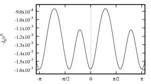


The sign in front of must be negative to achieve the desired extrema as minima rather than maxima. The other terms in the Higgs potential, Eq. (50), are independent of , depending only on the radial function . Hence, it is clear that Eq. (50) has the global minima we require. Figure 3 shows a contour plot of the Higgs potential for a certain parameter choice illustrating this conclusion. It is important to realise that although the minima and [similarly and ] look as though they are disconnected by , this is just an illusion created by only plotting the two-dimensional slice through the -dimensional adjoint representation space. Minima with opposite parities are definitely disconnected from each other.1010 10 While it is certainly true that the is not a subgroup of , so that in general and are disconnected from each other, one may worry that there is nevertheless an transformation that takes the specific configuration to . However, this is not the case. Explicit calculation of the invariant reveals a nonzero term. Hence, must be outside of . It does not matter that has been omitted from the Higgs potential, as it is a purely group-theoretic argument.

In the examples presented below, we further simplify the Higgs potential by setting as this term does not play an important role. It is then easy to show that at the degenerate minima,
| (59) |
so we must take , and that the value of at the minima is
| (60) |
The latter must be subtracted from the potential
| (61) |
to produce finite energy-densities for the domain wall configurations. Figure 3 is a contour plot of the potential energy showing the four degenerate global minima.
Having understood the global minima, we may now solve the Euler-Lagrange equations
| (62) |
using those VEVs as boundary conditions. Numerical solutions for CoS domain walls interpolating between at and at with two different parameter choices are displayed in Figure 4.


Figure 5 depicts non-CoS domain wall solutions for the same parameter choices. The function is zero, while interpolates between and in archetypal kink fashion. This means that the non-CoS configurations feel the large potential-energy maximum at , while the CoS configuration “skirts around” that central maximum. This immediately implies that the CoS solutions have lower energy density than the non-CoS solutions. Although they are in the same topological class, the CoS domain walls are stable while the non-CoS domain walls are unstable. Figure 6 shows a three-dimensional plot of the potential and where the two DW configurations sit with respect to the topography. There is a tall maximum at the origin, and a corrugated valley encircling it, with four low points at the VEVs. Figure 7 compares the energy densities of CoS and non-CoS domain walls.


IV.3 Fermion zero-mode localisation
The CoS domain wall solutions described above are a good starting point for the creation of domain-wall-brane models featuring -invariant effective -d theories for localised fields. To actually create such a model, fermions, additional Higgs bosons and gravitons have to be added. In this subsection, we demonstrate that a phenomenologically-acceptable fermion localisation pattern is obtained using the simplest possible mechanism. We explain why this is a remarkable result.
We simply Yukawa-couple a five-dimensional fermion multiplet in the of ,
| (63) |
to the adjoint scalar, as per
| (64) |
We now substitute in the background CoS DW configuration for and solve the resulting Dirac equations, which take the form
| (65) |
The notation signifies the component of the with the specified charges, as given in Eq. (26). The various components couple to different background field configurations,
| (66) |
given by the DW configuration and the charges.
The Dirac matrices are . We search for separated-variable solutions
| (67) |
demanding that have definite chirality, , and obey the -d massless Dirac equation, . The solution for a profile is well known:
| (68) |
where is a normalisation factor. For the profile to represent localisation, it must be square-integrable with respect to . For this to happen, must pass through zero. If so and it is an increasing function of (kink-like), then a left-(right-)handed zero-mode occurs for . If it passes through zero as a decreasing function (antikink-like), then a left-(right-)handed zero-mode occurs for .


Figure 8 show the kink-like functions for the two parameter choices we have been using as examples. Let us take to be negative:
| (69) |
Using the notation once again for the fermion multiplets, the following displays these functions and states the localisation outcome, which is either “localised as left-handed (LH) zero-mode” or “localised as right-handed (RH) zero-mode” or “delocalised”:
| (70) |
The two ’s are delocalised because the associated field never goes through zero. The and the are localised at with opposite chiralities because their background fields are kink-like and antikink-like, respectively. The two singlets are localised at nonzero values, so the overall spectrum is “split”.
This is a remarkable outcome for two reasons. First, because the is localised RH, it is equivalent to a LH-localised . Thus the localised spectrum consists of LH zero-modes in the representation
| (71) |
in other words one standard family plus two singlet neutrinos. Second, apart from the extra singlet, all the exotic fermions in the of are delocalised and thus do not feature in the effective -d theory on the brane. These benign outcomes depend crucially on the boundary condition choice embodied by the CoS domain wall solution, including the minus sign.
Finally, there is an amusing aspect to this spectrum. It resembles a usual family plus an extra singlet. However, the LH , which is obtained from a -d , and the do not come from a of either or .
V Conclusion
We find it extremely encouraging that, in the context, the clash-of-symmetries idea leads to good outcomes for both gauge-boson localisation (assuming the Dvali-Shifman mechanism works) and fermion localisation; that is the main point of this paper.
In summary, we have established a general connection between the clash-of-symmetries mechanism for simultaneous brane-creation and internal-symmetry breaking with the Dvali-Shifman mechanism for gauge boson localisation. The two together provide a strong basis upon which to construct realistic domain-wall-brane models. These models should be compatible with type-2 Randall-Sundrum graviton localisation (see Ref. Dando et al. 2005 for a CoS-style toy model featuring a background warped metric).
More specifically, we have found a domain wall solution in an adjoint-Higgs model that produces an symmetry on the wall itself. In one half of the bulk, the symmetry is enhanced to , while in the other half of the bulk the enhancement is to . The unprimed and primed groups are differently-embedded but isomorphic subgroups of . Because the brane- is contained in both and , the Dvali-Shifman localisation of its gauge bosons follows. The simplest possible mechanism for fermion zero-mode localisation produces a realistic spectrum, an outcome that depends on the generic features of our domain wall configuration.
To complete a realistic model, one needs to add gravity (which is expected to be straightforward) and to arrange for the additional spontaneous symmetry breaking cascade . To achieve the latter, suitable additional Higgs multiplets need to be introduced, and their background field configurations have to be nonzero inside the domain wall to trigger the additional spontaneous symmetry breaking. An example of this kind of dynamical structure is described in Ref. Davies et al. 2007, where the dominant background domain-wall configuration breaks to , and then an additional Higgs field induces electroweak symmetry breaking inside the wall.
Acknowledgements.
RRV and AK were supported by the Australian Research Council, DPG by the Puzey Bequest to the University of Melbourne, and KCW in part by funds provided by the U.S. Department of Energy (D.O.E.) #DE-FG02-92ER40702. AD is supported in part by the Albert Einstein Chair in Theoretical Physics.Appendix A Full minimisation analysis
We do this in two steps. We first extend the Higgs potential minimisation analysis by adding a third adjoint component, associated with the Cartan sub-algebra generator identified as weak hypercharge . This is useful because the result can be graphically visualised, and it reveals a third embedding of that is related to the two embeddings used in the main body of the text. In the second step, we report on a numerical study of the whole six-dimensional Cartan subspace.
The truncated multiplet is thus first increased to
| (72) |
where
| (73) |
have been normalised as per
| (74) |
The sextic invariant is
| (75) |
To visualise its structure, we go to a spherical-polar decomposition
| (76) |
which produces
| (77) | |||||
Figure 9 plots as a function of and . The plane is the line , along which the VEVs and can be seen. Degenerate with them are two more VEVs with , located at
| (78) |
and
| (79) |
The first VEV corresponds to a nonzero value for the adjoint component associated with the generator , where
| (80) |
As the notation suggests, this minimum breaks to yet a third differently-embedded subgroup which we can call , with negative parity: . The second VEV is just .

The three groups , and share a common subgroup, but the contained in is not a subgroup of (this is obvious, since contains an admixture of which is a generator of that ). One can imagine a domain-wall junction configuration that utilises all three of these embeddings for boundary conditions, but such a model would have a similar photon and -boson leakage problem as the warm-up example of Sec. III.
The functions , and have exactly the same qualitative structure as . Thus , and will be the degenerate global minima for a large class of potentials. The quadratic invariant is -independent,
| (81) |
so one can simply add appropriate terms to the potential to ensure it is bounded from below, and to generate a definite value for at the global minima. The positions of the global minima are determined entirely from the angular structure of the non-isotropic terms.
One can extend the analysis to all six Cartan components using a six-dimensional hyperspherical polar decomposition. The six fields are represented by one modulus, , four zenith angles and one azimuthal angle . Because the group theoretic character of an extremum is determined entirely from the angular structure of the invariants, a numerical study can readily be performed on the finite domain . This study confirmed that the VEVs are the global minima of and . The additional field dimensions simply revealed more degenerate vacua, corresponding to extra embeddings of in . These new embeddings must correspond, physically speaking, to choosing different subgroups for colour and isospin. The total number of extrema was found to be , consisting of -related pairs. This implies that, overall, there are embeddings of in . Though we shall not display the results here, we have analytical expressions for the linear combinations of Cartan generators that correspond to these VEVs. In the breakdown , these linear combinations turn out to be correlated with the choice of which component to assign as the singlet in the decomposition. A deeper reason for the number is perhaps the following: according to the maximal subgroup of , there are three independent choices for the colour group. The weak-isospin group can then be selected as the , or spin subgroup of either of the two remaining ’s. This gives choices for embeddings. According to our previous analysis, each is contained in the intersection of three different ’s, which suggests there should be embeddings of . However, recognising that contains an subgroup, we see that the correct number of independent embeddings is actually .
References
- Rubakov and Shaposhnikov (1983) V. A. Rubakov and M. E. Shaposhnikov, Phys. Lett. B125, 136 (1983).
- Akama (1983) K. Akama, Lecture Notes in Physics, Berlin Springer-Verlag 176, 267 (1983).
- Visser (1985) M. Visser, Phys. Lett. B159, 22 (1985).
- Gibbons and Wiltshire (1987) G. W. Gibbons and D. L. Wiltshire, Nucl. Phys. B287, 717 (1987).
- Arkani-Hamed et al. (1998) N. Arkani-Hamed, S. Dimopoulos, and G. R. Dvali, Phys. Lett. B429, 263 (1998).
- Antoniadis (1990) I. Antoniadis, Phys. Lett. B246, 377 (1990).
- Antoniadis et al. (1998) I. Antoniadis, N. Arkani-Hamed, S. Dimopoulos, and G. Dvali, Phys. Lett. B436, 257 (1998).
- Randall and Sundrum (1999a) L. Randall and R. Sundrum, Phys. Rev. Lett. 83, 3370 (1999a).
- Randall and Sundrum (1999b) L. Randall and R. Sundrum, Phys. Rev. Lett. 83, 4690 (1999b).
- Gremm (2000) M. Gremm, Phys. Lett. B478, 434 (2000).
- DeWolfe et al. (2000) O. DeWolfe, D. Z. Freedman, S. S. Gubser, and A. Karch, Phys. Rev. D62, 046008 (2000).
- Davidson and Mannheim (2000) A. Davidson and P. D. Mannheim (2000), eprint hep-th/0009064.
- Davies et al. (2007) R. Davies, D. P. George, and R. R. Volkas (2007), eprint arXiv:0705.1584[hep-ph].
- Davidson et al. (2002) A. Davidson, B. F. Toner, R. R. Volkas, and K. C. Wali, Phys. Rev. D65, 125013 (2002).
- Rozowsky et al. (2004) J. S. Rozowsky, R. R. Volkas, and K. C. Wali, Phys. Lett. B580, 249 (2004).
- Dando et al. (2005) G. Dando, A. Davidson, D. P. George, R. R. Volkas, and K. C. Wali, Phys. Rev. D72, 045016 (2005).
- Shin and Volkas (2004) E. M. Shin and R. R. Volkas, Phys. Rev. D69, 045010 (2004).
- Pogosian and Vachaspati (2000) L. Pogosian and T. Vachaspati, Phys. Rev. D62, 123506 (2000).
- Vachaspati (2001) T. Vachaspati, Phys. Rev. D63, 105010 (2001).
- Pogosian and Vachaspati (2001) L. Pogosian and T. Vachaspati, Phys. Rev. D64, 105023 (2001).
- Dvali and Shifman (1997a) G. Dvali and M. Shifman, Nucl. Phys. B504, 127 (1997a).
- Dvali and Shifman (1997b) G. R. Dvali and M. A. Shifman, Phys. Lett. B396, 64 (1997b).
- Jackiw and Rebbi (1976) R. Jackiw and C. Rebbi, Phys. Rev. D13, 3398 (1976).
- Rubakov (2001) V. A. Rubakov, Phys. Usp. 44, 871 (2001).
- Creutz (1979) M. Creutz, Phys. Rev. Lett. 43, 553 (1979).
- ’t Hooft (1976) G. ’t Hooft, in High Energy Physics, Proceedings of the EPS International Conference, Palermo 1975, ed. A Zichichi, Editrice Compositori, Bologna (1976).
- Mandelstam (1976) S. Mandelstam, Phys. Rep. C23, 245 (1976).
- Arkani-Hamed and Schmaltz (1999) N. Arkani-Hamed and M. Schmaltz, Phys. Lett. B450, 92 (1999).
- Dubovsky and Rubakov (2001) S. L. Dubovsky and V. A. Rubakov, Int. J. Mod. Phys. A16, 4331 (2001).
- Demaria and Volkas (2005) A. Demaria and R. R. Volkas, Phys. Rev. D71, 105011 (2005).
- Dynkin (1952) E. Dynkin, Mat. Sb. 30, 349 (1952).
- Li (1974) L.-F. Li, Phys. Rev. D9, 1723 (1974).
- Kaymakcalan et al. (1986) O. Kaymakcalan, L. Michel, K. C. Wali, W. D. McGlinn, and L. O’Raifeartaigh, Nucl. Phys. B267, 203 (1986).
- Bando and Kugo (1999) M. Bando and T. Kugo, Prog. Theor. Phys. 101, 1313 (1999).
- Bando et al. (2000) M. Bando, T. Kugo, and K. Yoshioka, Prog. Theor. Phys. 104, 211 (2000).
- Anderson and Blazek (2000) G. W. Anderson and T. Blazek, J. Math. Phys. 41, 4808 (2000).
- Maekawa and Yamashita (2003) N. Maekawa and T. Yamashita, Phys. Lett. B567, 330 (2003).
- Racah (1950) G. Racah, Lincei. Rend. Sci. Fis. Mat. Nat. 8, 108 (1950).
- Harvey (1980) J. A. Harvey, Nucl. Phys. B163, 254 (1980).