On the Capacity of Interference Channels with
One Cooperating Transmitter

Two-sender, two-receiver channel models allow for various forms of transmitter cooperation. When senders are unaware of each other’s messages, we have the interference channel [1, 2]. In wireless networks, the broadcast nature of the wireless medium allows nodes to overhear transmissions and possibly decode parts of other users’ messages. An encoder that has such knowledge can use it to improve its own rate and the other user’s rate. The level of cooperation and performance improvement will depend on the amount of information the encoders share. In the interference channel, rate gains from the transmitter cooperation were demonstrated in [3].

Channel models with cooperating nodes are of interest also for networks with cognitive users. Cognitive radio [4] technology is aimed at developing smart radios that are both aware of and adaptive to the environment. Such radios can efficiently sense the spectrum, decode information from detected signals and use that knowledge to improve the system performance. This technology motivates information-theoretic models that try to capture the cognitive radio characteristics. In that vein, this paper considers a two-sender, two-receiver channel model in which, somewhat idealistically, we assume that cognitive capabilities allow one user to know the full message of the other encoder, as shown in Fig. 1. Existing encoding schemes can bring different rate gains that depend on the channel characteristics and topology, making it challenging to determine the capacity even for special cases. This paper is a step along this path. It would further be interesting to extend the existing results to large networks with cooperating encoders.

Investigating the capacity region of the channel model we consider is the focus of much recent work. In particular, the interference channel with one cooperating encoder was dubbed the cognitive radio channel and achievable rates were presented in [3, 5]. A general encoding scheme was also proposed more recently in [6]. The capacity region for the Gaussian case of weak interference was determined in [7] and [8]. The results of [7, 8] were extended to the Gaussian MIMO cognitive radio network and shown to achieve the sum-capacity in [9]. Related work can also be found in [10, 11]. However, the conclusions of [9] do not immediately apply to the single-antenna cognitive radio channel. In this paper, we present a scheme that generalizes those in [7]-[12]. The scheme is similar to the one in [6]: as in [6] and [3], an encoder uses rate-splitting [2] to enable the other receiver to decode part of the interference; the cognitive transmitter cooperates in sending the other user’s message to its intended receivers and uses Gel’fand-Pinsker (GP) binning [13] to reduce interference to its own receiver. The key difference of our contribution to the prior work is in the way the binning is performed. An overview of the encoding scheme is given in the next section. The encoding scheme is derived in Section IV, compared to other results and adapted for Gaussian channel in Section VI.

In Section V, we present two outer bounds for the interference channel with one cooperating encoder. The first bound is based on the Nair-El Gamal broadcast outer bound, [14]. It has the same mutual information expression as the one in [14], the only difference is in the input distribution over which the optimization is performed. The bound thus reflects the resemblance of the considered channel to the broadcast channel (BC), and the difference given by the fact that encoder $2$ has only partial knowledge of messages sent in the channel. We then present an outer bound for the strong interference case that is of the same form as the one in [15, Sect.V], and compare it to the achievable rate region in Gaussian channels. Results also demonstrate an improvement compared to the general scheme of [6].

The considered channel model has elements of both the interference channel (IC) and the broadcast channel (BC). Encoding techniques developed for either of them are therefore potentially useful. If the message $W_{2}$ of encoder $2$ was not known at the cognitive encoder, the considered channel would reduce to the interference channel (IC). The best achievable rate region for the IC, [16], is achieved by rate-splitting [2]: each encoder divides its message into two parts and encodes each of them with a separate codebook. This allows receivers to decode one of the two sub-messages of the other user’s and cancel a part of the interference that it would otherwise create. Rate-splitting in the cognitive radio channel model was applied in [3, 6]. In this paper, rate-splitting is performed at the cognitive encoder.

Additional knowledge allows the cognitive encoder to employ a number of techniques in addition to rate-splitting. In particular, to improve the rate for the noncognitive communicating pair, the cognitive encoder can cooperate by encoding $W_{2}$ to help convey it to the other decoder. On the other hand, any signal carrying information about $W_{2}$ creates interference to the cognitive encoder’s receiver. This interference is known at the cognitive transmitter and the precoding technique, i.e. Gel’fand-Pinsker binning [13] and, specifically, dirty-paper coding (DPC) [17] in Gaussian channels, can be employed. In fact, GP binning is crucial for the cognitive radio channel: together with cooperation, it leads to capacity in certain scenarios, [7, 8, 9]. It is not surprising that DPC brings gains in the Gaussian cognitive radio channel: if the non-cognitive encoder is silent, we have the broadcast channel from the cognitive encoder to two receivers, for which dirty-paper coding is the optimal strategy [18, 19].

In general, however, there are two differences at the cognitive encoder from the classical GP setting. First, the interference carries useful information for receiver $2$. Second, the interference is a codebook of some rate and can thus have lower entropy than in the GP setting. As we will see in Sect. II-B, the latter can be exploited to achieve a higher rate.

We note that due to rate-splitting, there is a common part of $W_{1}$ decoded at the both receivers and precoded against interference. Since the signal carrying this common message experiences different interference at the two receivers, we use the ideas of [20] and [21] that respectively extend [13] and [17] to channels with different states non-causally known to the encoder. In the Gaussian channel, dirty paper coding is generalized to carbon-copying onto dirty paper [21] to adjust to the interference experienced at both receivers.

Consider a channel with finite input alphabets ${\cal X}_{1},{\cal X}_{2}$, finite output alphabets ${\cal Y}_{1},{\cal Y}_{2}$, and a conditional probability distribution $p(y_{1},y_{2}|x_{1},x_{2})$, where $(x_{1},x_{2})\in{{\cal X}}_{1}\times{{\cal X}}_{2}$ are channel inputs and $(y_{1},y_{2})\in{{\cal Y}}_{1}\times{{\cal Y}}_{2}$ are channel outputs. Each encoder $t$, $t=1,2$, wishes to send a message $W_{t}\in\{1,\ldots,M_{t}\}$ to decoder $t$ in $N$ channel uses. Message $W_{2}$ is also known at encoder $1$ (see Fig. 1). The channel is memoryless and time-invariant in the sense that

for all $n$, where $X_{1},X_{2}$ and $Y_{1},Y_{2}$ are random variables representing the respective inputs and outputs, ${\bar{w}}=[w_{1},w_{2}]$ denotes the messages to be sent, and $x_{t}^{n}=\begin{bmatrix}x_{t,1},&\ldots,&x_{t,n}\end{bmatrix}$. We will follow the convention of dropping subscripts of probability distributions if the arguments of the distributions are lower case versions of the corresponding random variables.

An $(M_{1},M_{2},N,P_{e})$ code has two encoding functions

two decoding functions

and an error probability

where, for $t=1,2$, we have

A rate pair $(R_{1},R_{2})$ is achievable if, for any $\epsilon>0$, there is an $(M_{1},M_{2},N,P_{e})$ code such that

The capacity region of the interference channel with a cooperating encoder is the closure of the set of all achievable rate pairs $(R_{1},R_{2})$.

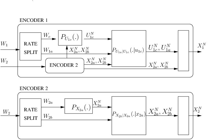
To obtain an inner bound, we employ rate splitting. We let

for nonnegative $R_{1a},R_{c},R_{2a},R_{2b}$ which we now specify.

In the encoding scheme, encoder $2$ uses superposition coding with two codebooks $X^{N}_{2a},X^{N}_{2b}$. Encoder $1$ repeats the steps of encoder $2$ and adds binning: it encodes the split message $W_{1}$ with two codebooks which are Gel’fand-Pinsker precoded against $X^{N}_{2a},X^{N}_{2b}$. In particular:

1. 1.

   Binning against $X^{N}_{2a},X^{N}_{2b}$ is used to create a codebook $U^{N}_{1c}$ of common rate $R_{c}$.

2. 2.

   Binning against $X^{N}_{2a},X^{N}_{2b}$ conditioned on $U_{1c}$ is used to create a codebook $U^{N}_{1a}$ with private rate $R_{1a}$.

The encoding structure is shown in Fig. 4.

We have the following result.

To illustrate obtained results more concretely, we next consider the Gaussian interference channel described by

where $Z_{t}\sim[0,1]$ and $E[X_{t}^{2}]\leq P_{t}$, $t=1,2$. In the case of weak interference, i.e., $b\leq 1$, the capacity region was determined in [7, 8].

We next evaluate the rates of Thm. 1 for the special case $X_{2a}=\emptyset$ and $Q=\emptyset$. Rates of Thm.1 for this case reduce to

To simplify (46), we express the conditional entropies in terms of joint entropies, recall that $R_{1}=R_{c}+R_{1a}$, and apply Fourier-Motzkin elimination to obtain

It is interesting to evaluate the rates of Thm. 2 achieved with sequential decoding for $X_{2a}=\emptyset,Q=\emptyset$ as was done for joint decoding in (46). This evaluation results in

We evaluated region (47) for

where ${\cal N}[0,\sigma^{2}]$ denotes the normal distribution with variance $\sigma^{2}$, and $0\leq\alpha,\beta\leq 1$ and $0\leq\lambda_{1},\lambda_{2}$. Parameters $\alpha$ and $\beta$ determine the amount of power that the cognitive user dedicates respectively for cooperation ($1-\alpha$) and for sending the common message.

We compared the achievable region (47) to the outer bound of Thm. 5 which in Gaussian channels is given by the following corollary:

Fig. 5 shows the achievable rate region (47) and the outer bound (50) for channel gain values $a^{2}=0.3$, $b^{2}=2$ and equal powers $P_{1}=P_{2}=6$. We observe higher rates of Thm. 1 compared to that of [6, Thm. $5$].

When the encoder $2$ does not transmit (i.e. $P_{2}=0$), the channel reduces to the broadcast channel in which there is only the cooperating encoder communicating to the two receivers. The rates achieved in the BC are also shown. Unlike the BC channel rate region, the interference channel with one cooperating encoder region is flat for smaller values of $R_{2}$, reflecting the fact that for smaller values of $R_{2}$ a cognitive transmitter does not need to cooperate. It can instead use its full power to precode and transmit $W_{1}$ at the single-user rate as if the second user was not present. It starts cooperating only for higher $R_{2}$. At $R_{1}=0$, the cooperating encoder fully helps encoder $2$, i.e. $\alpha=0$ and user $2$ benefits from the coherent combining gain as indicated by the rate expression

The achievable rates come very close to the outer bound, especially for larger values of $R_{2}$, in the regime where the cognitive encoder dedicates more of its power to cooperate.

Fig. 6 shows achievable rates for different values of power $P_{2}$ and fixed power $P_{1}$. As $P_{2}$ decreases, the performance gets closer to the rate achieved in the BC with only the cooperating encoder transmitting to the two receivers. Since in the BC encoder $2$ is not present, the rate region does not depend on $P_{2}$ and is given by the dashed line. Fig. 7 shows the effect of reducing power at the cognitive encoder, keeping $P_{2}$ constant. This has a higher impact, drastically reducing rate $R_{1}$.

For the Gaussian channel, the rates achieved with sequential encoding (48) can be evaluated for the choice of random variables $X_{2},X_{1},U_{1a},X_{1a}$ as in (49). $U_{1c}$ carries a common message and is to be precoded against interference. Since the two channels from encoder $1$ to the two receivers experience different interference, the carbon-copy method of [21] can be used. More details on this approach are presented in [12].

Fig. 8 shows the performance of the two decoding schemes given the channel gain values $a$ and $b$ for which the performance differs significantly.

We have developed an encoding strategy for the interference channel with one cooperating encoder that generalizes previously proposed encoding strategies. We evaluated its performance and compared it to the performance of other schemes, focusing on the Gaussian channel. A comparison with [3] would be an interesting next step. It is unclear whether our strategy generalizes the scheme in [3], or whether a combination of the two techniques would achieve higher rates. We also compared the proposed scheme to the outer bound that we developed for the strong interference regime. We further developed a new outer bound that extends the Nair-El Gamal broadcast outer bound. Evaluating this bound for specific channels such as Gaussian may prove useful.

The cognitive radio channel shares some characteristics of both interference channels and broadcast channels. Combining encoding strategies developed for either of the two channel models therefore seems a natural approach. However, the optimality of a particular encoding scheme seems to be in part dictated by the channel conditions: for the Gaussian channel in which decoder $2$ experiences weak interference, dirty-paper coding is capacity achieving. On the other hand, strong interference conditions may allow the cognitive receiver to decode the message not intended for him and therefore DPC against that message is not needed; superposition coding and rate-splitting achieve capacity. An even simpler scheme suffices when both receivers experience strong interference and can both decode the two messages. Neither DPC nor rate-splitting is needed; superposition coding is capacity-achieving. The encoding scheme presented in this paper is a combination of rate-splitting, GP binning and superposition coding. We believe that this general encoding scheme may be capacity-achieving for certain special cases related to the channel or specific encoding/decoding constraints. Finding such special cases is a topic of ongoing investigation

References

• [1] H. Sato, “Two user communication channels,” IEEE Trans. Inf. Theory, vol. 23, no. 3, pp. 295–304, May 1977.
• [2] A. B. Carleial, “Interference channels,” IEEE Trans. Inf. Theory, vol. 24, no. 1, pp. 60–70, Jan. 1978.
• [3] N. Devroye, P. Mitran, and V. Tarokh, “Achievable rates in cognitive radio channels,” IEEE Trans. Inf. Theory, vol. 52, no. 5, pp. 1813–1827, May 2006.
• [4] J. Mitola, Cognitive Radio Architecture. John Wiley Sons, Inc., 1991.
• [5] N. Devroye, P. Mitran, and V. Tarokh, “Limits on communications in a cognitive radio channel,” in IEEE Comm. Magazine, vol. 44, no. 6, June 2006, pp. 44–49.
• [6] J. Jiang and Y. Xin, “On the achievable rate regions for interference channels with degraded message sets,” IEEE Trans. Inf. Theory, submitted, Apr. 2007.
• [7] W. Wu, S. Vishwanath, and A. Arapostathis, “On the capacity of Gaussian weak interference channels with degraded message sets,” in Proc. Conf. Inf. Sciences and Systems (CISS), also submitted to IEEE Trans. Inf. Theory, Mar. 2006.
• [8] A. Jovičić and P. Viswanath, “Cognitive radio: An information-theoretic perspective,” in Proc. IEEE Int. Symp. Inf. Theory, also submitted to IEEE Trans. Inf. Theory, http://www.arxiv.org/pdf/0604/0604107v2.pdf, July 2006, pp. 2413–2417.
• [9] S. Sridharan and S. Vishwanath, “On the capacity of a class of MIMO cognitive radios,” in IEEE Information Theory Workshop (ITW 2007), Lake Tahoe, Ca, USA, Sept. 2007.
• [10] D. Tuninetti, “The interference channels with generalized feedback,” in IEEE Proc. Int. Symp. Inf. Th., jun 2007.
• [11] Y. Cao, B. Chen, and J. Zhang, “A new achievable rate region for interference channels with common information,” in Proc. IEEE Wireless Comm. and Networking Conf., 2007.
• [12] I. Marić, A. Goldsmith, G. Kramer, and S. Shamai(Shitz), “On the capacity of interference channels with a cognitive transmitter,” in Information Theory and Applications (ITA), http://ita.ucsd.edu/workshop/07/files/paper/paper431.pdf, Jan. 2007.
• [13] S. I. Gel’fand and M. S. Pinsker, “Coding for channel with random parameters,” Problemy Peredachi Informatsii, vol. 9, no. 1, pp. 19–31, 1980.
• [14] C. Nair and A. E. Gamal, “An outer bound to the capacity region of the broadcast channel,” IEEE Trans. Inf. Theory, vol. 53, no. 1, pp. 350–355, Jan. 2007.
• [15] I. Marić, R. D. Yates, and G. Kramer, “Capacity of interference channels with partial transmitter cooperation,” IEEE Trans. Inf. Theory, vol. 53, no. 10, Oct. 2007.
• [16] T. Han and K. Kobayashi, “A new achievable rate region for the interference channel,” IEEE Trans. Inf. Theory, vol. 27, no. 1, pp. 49–60, Jan. 1981.
• [17] M. H. M. Costa, “Writing on dirty paper,” IEEE Trans. Inf. Theory, vol. 29, no. 3, pp. 439–441, May 1983.
• [18] H. Weingarten, Y. Steinberg, and S. Shamai(Shitz), “The capacity region of the Gaussian multiple input multiple output broadcast channel,” IEEE Trans. Inf. Theory, vol. 52, no. 9, pp. 3936–3964, Sept. 2006.
• [19] S. Vishwanath, N. Jindal, and A. Goldsmith, “Duality, achievable rates and sum rate capacity of gaussian MIMO broadcast channels,” IEEE Trans. Inf. Theory, vol. 49, no. 10, pp. 2658–2668, Oct. 2003.
• [20] P. Mitran, N. Devroye, and V. Tarokh, “On compound channels with side-information at the transmitter,” IEEE Trans. Inf. Theory, vol. 52, no. 4, pp. 1745–1755, Apr. 2006.
• [21] A. Khisti, U. Erez, A. Lapidoth, and G. W. Wornell, “Carbon copying onto dirty paper,” IEEE Trans. Inf. Theory, vol. 53, no. 5, pp. 1814–1827, May 2007.
• [22] J. Jiang, Y. Xin, and H. Garg, “Interference channels with common information,” IEEE Trans. Inf. Theory, submitted.
• [23] Y. Liang, A. Somekh-Baruch, V. Poor, S. Shamai(Shitz), and S. Verdú, “Cognitive interference channels with confidential messages,” in 45th Annual Allerton Conference on Communication, Control and Computing, Allerton House, Monticello, IL, USA, Sept. 2007.
• [24] T. Cover, Y. Kim, and A. Sutivong, “Channel capacity and state uncertainty reduction for state-dependent channels,” in Proc. IEEE Int. Symp. Inf. Theory, June 2007.
• [25] ——, “Simultaneous communication of data and state,” http://arxiv.org/PScache/cs/pdf/0703/0703005v1.pdf, 2007.
• [26] A. Jovičić and P. Viswanath, “Cognitive radio: An information-theoretic perspective,” IEEE Trans. Inf. Theory, submitted, http://www.arxiv.org/pdf/cs.IT/0604107.pdf, 2006.
• [27] S. Lall, Advanced Topics in Computation for Control. Lecture notes, Stanford University, 2004.
• [28] F. M. J. Willems, “The discrete memoryless multiple access channel with cribbing encoders,” IEEE Trans. Inf. Theory, vol. 31, no. 3, pp. 313–327, May 1985.
• [29] T. Cover and J. Thomas, Elements of Information Theory. John Wiley Sons, Inc., 1991.
• [30] G. Kramer, Multiple User Information Theory, lecture notes. unpublished, 2006.