Two-parameter model predictions and $\theta$-point crossover for linear-polymer solutions

The main purpose of the present paper is the determination of the crossover functions for the quantities defined in Sec. III. We consider five different values of $z$, which we denote by $z_{1}$, $\ldots$, $z_{5}$, which belong to the crossover region between ideal and good-solvent behavior. Explicitly we use $z_{1}=0.056215$, $z_{2}=0.148726$, $z_{3}=0.32165$, $z_{4}=0.728877$, and $z_{5}=2.50828$. They were chosen so that $A_{2}(z_{n})\approx n$ (remember that $A_{2}(z)$ varies between 0 and 5.50). In order to compute the TPM value for each $z_{i}$, we perform several simulations at values $(w_{ij},N_{ij})$ such that $w_{ij}N_{ij}^{1/2}=(2\pi/3)^{3/2}z_{i}$, choosing $N_{ij}$ between 100 and 8000. Then, we fit each universal quantity $Q$ with the theoretically expected behavior:BD-79; BN-97; foot-TPM

$$Q(w_{ij},N_{ij})=Q^{*}(z_{i})+N_{ij}^{-1/2}b_{Q}(z_{i})+N_{ij}^{-1}c_{Q}(z_{i}).$$

(27)

The TPM result corresponds to the leading term $Q^{*}(z_{i})$. In order to detect additional scaling corrections that are not taken into account by the fit ansatz (27), we have repeated the fit several times, each time including only data satisfying $N\geq N_{\rm min}$.

We illustrate the procedure by considering $A_{2}$. In Fig. 1 we plot $A_{2}(w,N)$ vs $N^{-1/2}$; for each $z$ we also plot the function $Q^{*}+N^{-1/2}b_{Q}$ obtained in the fit of all data ($N_{\rm min}=100$) to Eq. (27). The data points follow the expected behavior quite precisely, with very small $N^{-1}$ corrections. Note that an extrapolation is always needed except for very small values of $z$. Estimates of $A_{2}(z)$ are reported in Table 1 for different values of $N_{\rm min}$. No systematic deviations are observed. We take the results corresponding to $N_{\rm min}=500$ as our final results. They are reported in Table 2. We have applied the same analysis to $A_{3}$, $A_{4}$, $A_{ge}$, $A_{gH}$, $S_{n,g}$, $S_{n,e}$, $S_{n,H}$ ($n=1,2$). The results corresponding to $N_{\rm min}=500$ are reported in Table 2.

Finally, we determine the swelling factors. We consider $6\hat{R}_{g}^{2}/N$, $\hat{R}_{e}^{2}/N$, and $k_{H}\sqrt{N}/\hat{R}_{H}$ ($k_{H}=2^{-7/2}(3\pi)^{1/2}$). The corresponding quantities are reported in Fig. 2. Their behavior with $N$ at fixed $z$ is perfectly consistent with Eq. (27). Therefore, we have performed the same fits as before. The results are reported in Table 2.

We now use the results of Sec. IV.1, the good-solvent results of Refs. CMP-vir; CMP-raggi, and the small-$z$ results mentioned in Sec. III and in the Appendix, to obtain interpolation formulas that are valid for all values of $z$. We discuss in detail the virial coefficients; all other quantities are analyzed analogously.

For the second virial coefficient we wish to find an interpolation that satisfies the following properties: (i) for $z\to\infty$ it must satisfy $A_{2}(z)\to A_{2}^{*}=5.500$ [Eq. (8)]; (ii) for $z\to 0$ it must behave as $4\pi^{3/2}z(1-4.779663z)$ [Eq. (13)]; (iii) the interpolating curve should assume the values determined numerically and reported in Table 2. Since the results for $A_{2}(z)$ indicate that this function is monotonic, we take an interpolating function of the form

$$A_{2}(z)=4\pi^{3/2}z(1+d_{1}z+d_{2}z^{2}+d_{3}z^{3}+d_{4}z^{4})^{-1/4},$$

(28)

where $d_{i}$ are constants to be determined. The constant $d_{1}$ can be fixed to obtain the expansion (13) to order $z^{2}$: we obtain $d_{1}=19.1187$. The constant $d_{4}$ can be fixed by requiring $A_{2}(z=\infty)=A_{2}^{*}$, where $A_{2}^{*}$ is given in Eq. (8): this gives $d_{4}=268.96$. Then, we fit

$$\left[{4\pi^{3/2}z\over A_{2}(z)}\right]^{4}-1-d_{1}z-d_{4}z^{4}=d_{2}z^{2}+d_{3}z^{3}\;.$$

(29)

Using the five data reported in Table 2 we obtain $d_{2}=126.783$ and $d_{3}=331.99$. The interpolation formula is reported in Table 3. For $z\to\infty$, Eq. (28) gives

$$A_{2}(z)=5.500-1.6972/z+O(z^{-2})\;.$$

(30)

This expression is compatible with Eq. (12), taking into account thatBN-97 $2\Delta\approx 1.03$. It allows us to estimate $a_{2}$: $a_{2}\approx-1.7$. Of course, this is a very rough estimate. A careful determination would require $A_{2}(z)$ for much larger values of $z$ and a careful analysis of the corrections to the behavior (12). Expression (30) agrees with the field-theoretical result reported in Ref. Nickel-91, which predicts $a_{2}\approx 5.50\times(-0.30)\approx-1.65$.

We now compare the interpolation formula (28) with similar expressions that appear in the literature. We consider the expression reported in Ref. Schaefer-99 (Sec. 15.5.2):

$$A_{2}(z)={1\over 2}(4\pi)^{3/2}{0.182\tilde{z}(1+2.15\tilde{z}+0.82\tilde{z}^{2})^{-0.236}\over(1+1.32\tilde{z}+0.378\tilde{z}^{2})^{0.264}},$$

(31)

wherefoot-A2-Sch $z=0.182\tilde{z}$. Equation (31) has been obtained by using a sophisticated form of renormalized one-loop perturbation theory. By means of an extensive Monte Carlo simulation Ref. BN-97 obtained

$$A_{2}(z)={1\over 2}(4\pi)^{3/2}z(1+14.339z+60.30z^{2}+66.3z^{3})^{-1/3}.$$

(32)

Finally, we quote the field-theoretical expression of Ref. DF-84 for $\epsilon=1$:

$$A_{2}(z)={1\over 2}(4\pi)^{3/2}\left\{{\eta\over 8(1+\eta)}+{1\over 64}\left[\left(4\ln 2+{7\over 6}\right)\left({\eta\over 1+\eta}\right)^{2}+{21\eta\over 4(1+\eta)}\right]\right\},$$

(33)

with $\eta=256z/53$ (this relation is obtained by matching the small-$z$ behavior). Our result (28) is essentially identical to Eq. (32): differences are less than 0.3%. It is also in very good agreement with the field-theoretical result (31), differences being less than 1.5%. Eq. (33) is worse: the difference is of order 8% for $z=0.1$ and increases to 12% for large values of $z$.

Let us now discuss $A_{3}$. We will use an interpolation formula analogous to (28), setting

$$A_{3}(z)=1100.7z^{3}(1+d_{1}z+d_{2}z^{2}+d_{3}z^{3}+d_{4}z^{4})^{-3/4}.$$

(34)

The prefactor has been fixed by using Eq. (14). To determine the coefficients we use a strategy slightly different from that discussed for $A_{2}$, since we only know the leading small-$z$ behavior of $A_{3}$ and thus we cannot fix $d_{1}$ by using perturbation theory. Instead, we make use of the results of Ref. CMP-vir to obtain the large-$z$ behavior of $A_{3}(z)$. SinceCMP-vir $b_{3}=a_{3}/a_{2}=4.75$ [see Eq. (12)], Eqs. (30) and (9) give $A_{3}(z)\approx 9.80-8.062/z$ (again we use the approximation $2\Delta\approx 1$). If we require Eq. (28) to reproduce this expansion, we obtain $d_{3}=594.386$ and $d_{4}=541.906$. Finally, we fit the results of Table 2 to determine $d_{1}$ and $d_{2}$. The resulting expression is reported in Table 3.

Finally, we consider $A_{4}$. In this case we do not know $a_{4}/a_{2}$ and thus we use an interpolation formula with only three parameters:

$$A_{4}(z)=-29883.1z^{4}(1+d_{1}z+d_{2}z^{2}+d_{3}z^{3})^{-4/3}.$$

(35)

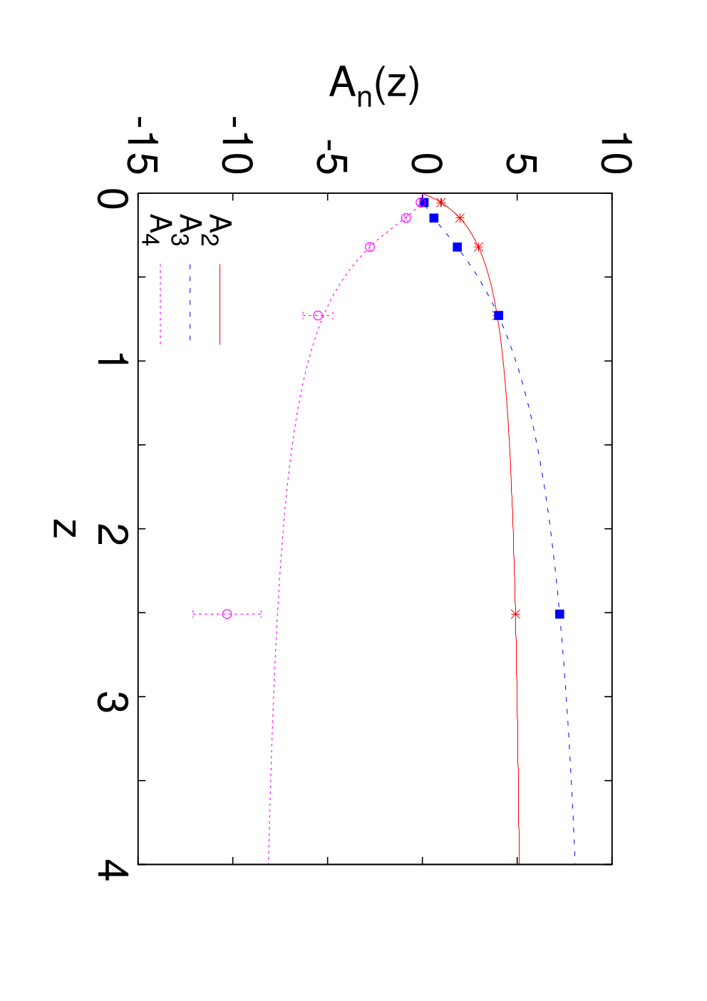
The prefactor has been fixed by using Eq. (15). The constant $d_{3}$ is fixed by using Eq. (10), $d_{1}$ and $d_{2}$ by fitting the numerical results of Table 2. The final expression is reported in Table 3. In Fig. 3 we report the crossover functions for $A_{2}$, $A_{3}$, $A_{4}$. They are monotonic and approach the good-solvent value for $z\gtrsim 5$.

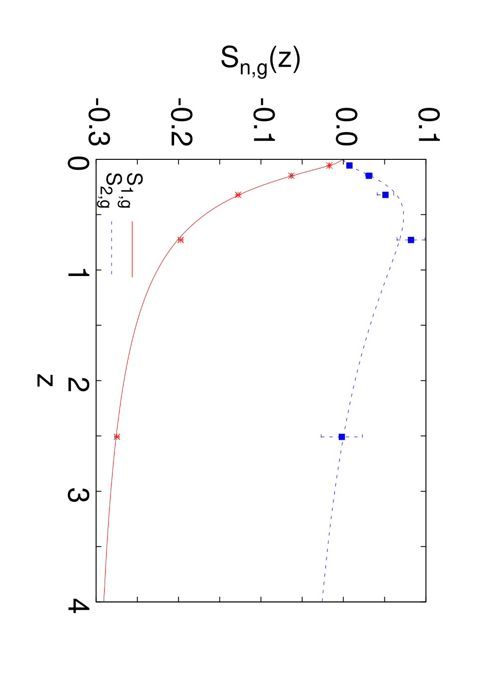
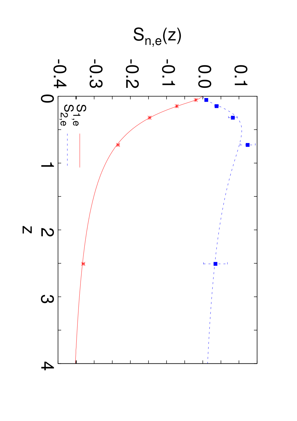
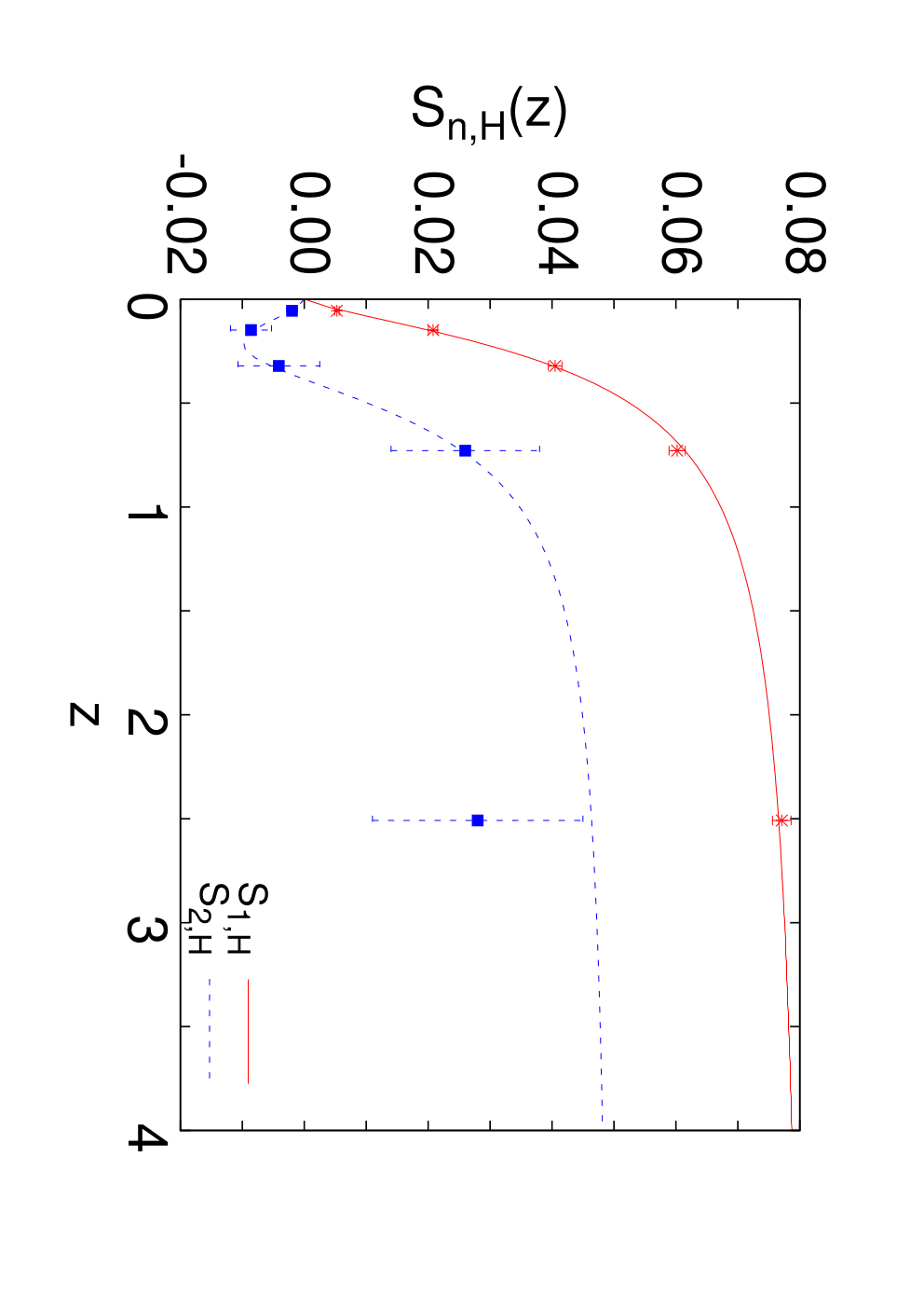
Similar analyses are performed for the density corrections to the radii. In this case, however, the crossover functions are not monotonic. For the second density correction, this is evident from the numerical data. For instance, $S_{2,g}$ and $S_{2,e}$ are first positive and increasing, in agreement with Eqs. (69), (74), reach a maximum for $0.5\lesssim z\lesssim 1$, and then decrease, converging to the good-solvent value which is negative. The density coefficient $S_{2,H}$ behaves in the opposite way, but note that, because of its definition, $S_{2,H}$ is equivalent in some sense to $-S_{2,e}$ and $-S_{2,g}$. For the first density correction the nonmonotonicity can be inferred by using the results of Ref. CMP-raggi. If $S_{1,\#}=S_{1,\#}^{*}(1+\lambda_{\#}z^{-2\Delta})$, we have $\lambda_{\#}A_{2}^{*}/a_{2}\approx-0.050$ for both $S_{1,e}$ and $S_{1,g}$ [$a_{2}$ is defined in Eq. (12)]. Using $a_{2}\approx-1.697$ [Eq. (30)], we obtain:

$$S_{1,g}\approx-0.3152-0.0049/z^{2\Delta},\qquad S_{1,e}\approx-0.3853-0.0059/z^{2\Delta}.$$

(36)

Thus, the first density correction vanishes for $z=0$, then decreases, becomes smaller than the good-solvent value, and eventually converges to it from below. This effect is however numerically very small and thus the nonmonotonic approach is in practice irrelevant. The nonmonotonic behavior requires interpolation formulas slightly different from those used for the virial coefficients. For instance, expressions like (28) cannot change sign and thus are unsuitable for $S_{2,\#}$. Our interpolations are reported in Table 3 and plotted in Fig. 4. Note that the interpolations of $S_{2,\#}$ are not very precise in the region $0.5\lesssim z\lesssim 1$, since here the functions change their behavior and we do not have enough data points to identify precisely where the functions reach their maximum.

Finally, let us consider the swelling factors. Because of Eq. (26), we use an interpolation of the form

$$\alpha_{\#}=(1+b_{1}z+b_{2}z^{2}+b_{3}z^{3})^{(2\nu-1)/3},$$

(37)

takingBN-97 $\nu=0.58758$. The coefficient $b_{1}$ is fixed by requiring $\alpha_{\#}$ to reproduce the small-$z$ behavior reported in the appendix, while $b_{2}$ and $b_{3}$ are obtained by interpolating the numerical data. The results are reported in Table 3 and shown in Fig. 5. Note that $\alpha_{e}$, $\alpha_{g}$, $\alpha_{H}$ behave in a very similar way, differences being tiny. For $\alpha_{g}$ we also show the prediction of Ref. BN-97, $\alpha_{g}=(1+7.286z+9.51z^{2})^{0.087583}$, and that of Ref. Schaefer-99, $\alpha_{g}=(1+1.32\tilde{z}+0.378\tilde{z}^{2})^{0.088}$, wherefoot-A2-Sch $z=0.182\tilde{z}$. The result of Ref. BN-97 is perfectly consistent with ours. The field-theoretical result [note that in Fig. 5 it can hardly be distinguished from our result for $\alpha_{e}(z)$] is slightly larger (1% at $z=5$): differences are mainly related to the different choice of the exponent $\nu$. Finally, for the end-to-end distance we mention the result of Ref. BN-97: $\alpha_{e}=(1+7.6118z+12.05135z^{2})^{0.087583}$. Again, this expression is in perfect agreement with ours.

Knowledge of the crossover functions for the lowest virial coefficients provides the osmotic pressure in the dilute regime in which $\Phi_{p}\lesssim 1$, where $\Phi_{p}$ is the polymer packing fraction,

$$\Phi_{p}\equiv{4\pi\hat{R}^{3}_{g}\over 3}c={4\pi\hat{R}^{3}_{g}\over 3}{N_{A}\over M}\rho,$$

(38)

$N_{A}$ the Avogadro number, $M$ the molar mass of the polymer, $c$ and $\rho$ the number density and the weight concentration, respectively. In Fig. 6 we report the compressibility factor $Z$ defined in Eq. (5) for several values of $z$ for $\Phi_{p}\lesssim 1$. In this range of concentrations the virial expansion converges quite well CMP-vir and thus our interpolations provide accurate estimates of $Z$ as a function of $z$ and $\Phi_{p}$.

In Ref. CMP-vir it was shown that a resummation of the virial expansion by using the known large-$\Phi_{p}$ behavior provides a reasonably accurate expression for $Z$ valid in the whole semidilute region. Here we apply the same method to the determination of the leading $z^{-2\Delta}$ correction to the good-solvent value. Since $A_{n}=A^{*}_{n}+a_{n}z^{-2\Delta}$ for large $z$, we can write

$$Z(z,N,c)\approx Z^{*}(N,c)+z^{-2\Delta}Z_{1}(N,c)\;.$$

(39)

The functions $Z^{*}(N,c)$ and $Z_{1}(N,c)$ depend on $c$ and $N$. However, for $N\to\infty$, the renormalization group predicts that they become universal functions of the packing fraction $\Phi_{p}$, so that

$$Z(z,N,c)\approx Z^{*}(\Phi_{p})+z^{-2\Delta}Z_{1}(\Phi_{p}).$$

(40)

The good-solvent function $Z^{*}(\Phi_{p})$ is reported in Ref. CMP-vir. We will now determine the function $Z_{1}(\Phi_{p})$. For this purpose we determine its large-$\Phi_{p}$ behavior. We expect

$$Z_{1}(\Phi_{p})\sim\Phi_{p}^{\alpha},\qquad\qquad\Phi_{p}\to\infty.$$

(41)

To fix $\alpha$, we note that $\Pi$ is a function of the monomer concentration $c_{m}\equiv cN$ but not of the degree of polymerization $N$ for $c\to\infty$ (and therefore also $c_{m}\to\infty$). Hence, $cz^{-2\Delta}\Phi_{p}^{\alpha}$ should be independent of $N$, once $c$ has been replaced by $c_{m}$. This condition implies

$$\alpha={\Delta+1\over 3\nu-1}.$$

(42)

In order to understand the region in the $(c,z)$ plane in which expansion (40) is valid, we must discuss the expected scaling behavior in the large-concentration limit for generic values of $z$. In the TPM the osmotic pressure satisfies the general scaling behaviorSchaefer-99

$${\Pi\over k_{B}T}=c{\cal P}(c\ell^{3}N^{3/2},z).$$

(43)

In the limit $z\to 0$ the Flory-Huggins theory applies: for large values of $c$, $\Pi$ is proportional to the square of the monomer concentration $c_{m}$ and to the interaction strength $w$, so that

$${\Pi\over k_{B}T}\sim wc_{m}^{2}\ell^{3}\sim cz(c\ell^{3}N^{3/2}).$$

(44)

For large $c$, the dependence on $N$ should disappear at fixed $c_{m}$ and $w$, so that the relevant scaling variable is $z/(c\ell^{3}N^{3/2})=w/(c_{m}\ell^{3})$. Therefore, we obtain the scaling behavior

$${\Pi\over k_{B}T}=zc^{2}\ell^{3}N^{3/2}f_{Z}\left({z\over c\ell^{3}N^{3/2}}\right),\qquad\qquad Z=zc\ell^{3}N^{3/2}f_{Z}\left({z\over c\ell^{3}N^{3/2}}\right).$$

(45)

The function $f_{Z}(x)$ is finite for $x\to 0$, while for $x\to\infty$, consistency with (40) implies

$\displaystyle f_{Z}(x)\approx a_{f}x^{(3\nu-2)/(3\nu-1)}(1+b_{f}x^{-\Delta/(3\nu-1)}).$

(46)

The value $f_{Z}(0)$ can be determined by noting that for $z\to 0$ we can write

$$Z\approx zc\ell^{3}N^{3/2}f_{Z}(0)=A_{2}c\hat{R}_{g}^{3}=4\pi^{3/2}zc(N/6)^{3/2}\ell^{3}.$$

(47)

This implies $f_{Z}(0)=(2\pi/3)^{3/2}/2$.

Eq. (45) indicates that, at fixed large $z$, the compressibility factor shows two different behaviors. If $\Phi_{p}$ is large but still $z\gg c\ell^{3}N^{3/2}$, $Z$ increases following Eq. (40). If the concentration is further increased, the argument of $f_{Z}(x)$ decreases and eventually $Z\approx zc\ell^{3}N^{3/2}f_{Z}(0)=3\sqrt{\pi}z\alpha_{g}^{-3}\Phi_{p}$, i.e. $Z$ becomes linear in the concentration. It is clear that this second regime cannot be obtained from extrapolations of results in the dilute region. We will thus consider only concentrations such that $z\gg c\ell^{3}N^{3/2}$, so that we can use Eq. (40).

To determine the osmotic pressure for densities in the semidilute regime satisfying $z\gg c\ell^{3}N^{3/2}$ we expand $A_{n}(z)=A_{n}^{*}+A_{n,1}/z$ for $z\to\infty$. Thus, we obtain for $z\to\infty$

	$\displaystyle Z$	$\displaystyle\approx$	$\displaystyle 1+1.31303\Phi_{p}+0.558533\Phi_{p}^{2}-0.122455\Phi^{3}$		(48)
		$\displaystyle+$	$\displaystyle{1\over z}\left(-0.405182\Phi_{p}-0.459468\Phi_{p}^{2}+0.0507105\Phi_{p}^{3}\right),$

which is consistent with (40) if we approximate $2\Delta\approx 1$. In Ref. CMP-vir we determined an interpolation formula for the leading term with the correct large-$\Phi_{p}$ behavior. Here we do the same for the correction term: we determine an interpolation formula that has the asymptotic behavior (41) for $\Phi_{p}\to\infty$ with $\alpha$ given by Eq. (42), and agrees with the previous expansion for $\Phi_{p}\to 0$. A simple expression satisfying these two properties is

$$-0.405182\Phi_{p}(1+2.30016\Phi_{p}+1.08734\Phi^{2}_{p})^{0.493}\;.$$

(49)

Combining this expression with that obtained in Ref. CMP-vir we obtain for the compressibility factor

	$\displaystyle Z$	$\displaystyle=$	$\displaystyle\left({1+1.52605\Phi_{p}+0.795366\Phi_{p}^{2}\over 1+0.5245\Phi_{p}}\right)^{1.311}$		(50)
			$\displaystyle-{0.405182\over z^{2\Delta}}\Phi_{p}(1+2.30016\Phi_{p}+1.08734\Phi^{2}_{p})^{0.493}.$

It is not possible to determine a priori, for each $z$, the density range $\Phi_{p}\lesssim\Phi_{p,\rm max}(z)$ in which Eq. (50) applies. For $\Phi_{p}=1$ we can compare expression (50) with the virial expansion (5) including the terms up to $n=4$. The relative difference is less than 5% (1%, 0.1% respectively) for $z\gtrsim 1.7$ (4, 12 respectively). Thus, for $\Phi_{p}=1$, Eq. (50) is substantially correct for $z\gtrsim 4$ and reasonably predictive for $z\gtrsim 2$. Accepting an error of 5% (it makes little sense to require a smaller error since our interpolation formulas cannot in any case be more precise than 5-10%; see the discussion reported in Ref. CMP-vir), we can set $\Phi_{p,\rm max}(z=2)=1$. An estimate of $\Phi_{p,\rm max}(z)$ for larger values of $z$ can be obtained by noting that

$$\Phi_{p,\rm max}(z)\sim z^{6\nu-2}\sim z^{2.53}.$$

(51)

Indeed, Eq. (50) is valid as long as $z\gg c\ell^{3}N^{3/2}\sim c\hat{R}_{g}^{3}\alpha_{g}^{-3}\sim\Phi_{p}\alpha_{g}^{-3}$. Hence, since $\alpha_{g}\sim z^{2\nu-1}$ for large $z$, we obtain Eq. (51). Therefore, with errors at most of 5% we expect the range to extend up to $\Phi_{p,\rm max}(z)\approx(z/2)^{2.53}$.

The prediction (50) for $\Phi_{p}\leq 10$ is reported in Fig. 7 for several values of $z$. It is clear that the results for $z=2$ do not extend beyond $\Phi_{p}=1$, since, by increasing $\Phi_{p}$, $Z$ begins to bend in an unphysical way. No such phenomenon is observed for $z\gtrsim 5$, which is therefore expected to be the range of $z$ in which (50) applies for $\Phi_{p}\lesssim 10$. This is in agreement with the estimate of $\Phi_{p,\rm max}(z)$ given above. Note that scaling corrections are quite large in the semidilute regime. For instance, consider $z=10$. Since $A_{2}/A_{2}^{*}=\Psi/\Psi^{*}=0.97$, in the dilute regime the solution is essentially in good-solvent conditions. For $\Phi_{p}=10$ we obtain $Z=31.3$ to be compared with the good-solvent value $Z_{GS}=35.8$: the pressure is lower by 14%, a significant deviation from the good-solvent value.

The considerations we have presented for the osmotic pressure can be generalized to the radii. Deep in the semidilute region, polymers behave like ideal chains and therefore $R^{2}$ behaves as

$$R^{2}=N\ell^{2}f_{R}(w/c_{m})=N\ell^{2}f_{R}\left({z\over c\ell^{3}N^{3/2}}\right),$$

(52)

with $f_{R}(0)\not=0$. As before, we focus on the deviations from the good-solvent regime. If $R$ is the end-to-end distance or the radius of gyration, corrections scale as $z^{-2\Delta}$ (this is not the case for the hydrodynamic radius which may show additional corrections proportional to DRSK-02; CMP-raggi $z^{4\nu-4}$). In order to obtain the behavior for large $c$ in the good-solvent regime we write

$$R^{2}=a_{R}\hat{R}^{2}\Phi_{p}^{\alpha_{1}}(1+b_{R}z^{-2\Delta}\Phi_{p}^{\alpha_{2}}),$$

(53)

and require this expression to be consistent with Eq. (52). This allows us to identify $\alpha_{1}$ and $\alpha_{2}$:

$$\alpha_{1}=-{2\nu-1\over 3\nu-1}\qquad\qquad\alpha_{2}={\Delta\over 3\nu-1}.$$

(54)

Using these expressions, we can now extrapolate our virial results to the whole semidilute region, obtaining (the leading terms already appear in Ref. CMP-raggi)

	$\displaystyle{R^{2}_{e}\over\hat{R}^{2}_{e}}$	$\displaystyle=$	$\displaystyle(1+0.801\Phi_{p}+0.37\Phi^{2}_{p})^{-0.115}-{1\over z^{2\Delta}}0.024\Phi_{p}(1+0.76\Phi_{p})^{-0.554},$		(55)
	$\displaystyle{R^{2}_{g}\over\hat{R}^{2}_{g}}$	$\displaystyle=$	$\displaystyle(1+0.655\Phi_{p}+0.28\Phi_{p}^{2})^{-0.115}-{1\over z^{2\Delta}}0.021\Phi_{p}(1+1.46\Phi_{p})^{-0.554}.$		(56)

As discussed before, these expressions are only valid for $z\ll c\ell^{3}N^{3/2}$. We do not present an extrapolation for $R_{H}$, because of the presence of two different corrections (one proportional to $z^{-2\Delta}$ and one proportional to $z^{4\nu-4}$, see Ref. DRSK-02), which make extrapolations of the form (53) incorrect. The results for $R_{g}^{2}/\hat{R}^{2}_{g}$ are shown in Fig. 8 for the same values of $z$ that occur in Fig. 7. Note that for large $z$, our extrapolation predicts $R_{g}^{2}/\hat{R}^{2}_{g}$ to decrease when $z$ decreases. This is consistent with the nonmonotonic behavior of $S_{1,g}(z)$ we mentioned in Sec. IV.2 and with the numerical results of Ref. CMP-raggi, which suggest a negative scaling correction for $S_{2,g}(z)$: $S_{2,g}(z)=-0.087-(0.003\pm 0.005)z^{-2\Delta}$. Of course, this behavior should eventually change, since $R_{g}^{2}/\hat{R}^{2}_{g}$ should converge to 1 as $z\to 0$.

For the radius of gyration corrections are less evident than in the case of $Z$. For instance, for $\Phi_{p}=10$ the relative difference between $R^{2}_{g}/\hat{R}^{2}_{g}$ for $z=10$ and for $z=\infty$ (good-solvent value) is only of 0.7%, indicating that the polymer size is less sensitive to the solvent quality far from the ideal-chain limit.

In the previous sections we have obtained predictions for the osmotic pressure and the radii in the TPM. We wish now to compare these results with those obtained by using field theory. We compare mainly with the results reported in Ref. Schaefer-99, which have been obtained by using renormalized one-loop perturbative expressions with a careful choice of the renormalization constants. In Fig. 9 we report the compressibility factor $Z$ as a function of $z$ for $\Phi_{p}=1$, i.e. for the largest value of the density at which the virial expansion is supposed to work. As we discussed in Ref. CMP-vir this expression should be quite accurate, deviations being at most of 1-2%. We also report the field-theoretical result, which is in perfect agreement with our estimate. For larger values of $\Phi_{p}$ we cannot use the virial expansion. Instead, we employ the approximate expression (50), which is valid only for large values of $z$. In Fig. 10 we report $Z$ in the range $0\leq\Phi_{p}\leq 10$ for two values of $z$: $z=9.90$ corresponding to $R\equiv 1-\Psi/\Psi^{*}=0.03$ and $z=5.79$ corresponding to $R=0.05$. We report our expression (50) and the field-theoretical prediction of Ref. Schaefer-99. For $R=0.03$, our result is in very good agreement with the field-theoretical one. On the other hand, for $R=0.05$, we observe significant differences for $\Phi_{p}\gtrsim 5$. In any case, these discrepancies are within the 5% error we expect on our extrapolations. Indeed, for $\Phi_{p}=5$ we predict $Z_{GS}=15.0$ and $Z(z=5)=12.9$ to be compared with the field-theory results $Z_{GS}=14.5$ and $Z(z=5)=12.7$; for $\Phi_{p}=10$ we obtain $Z_{GS}=35.9$ and $Z(z=5)=28.5$ to be compared with $Z_{GS}=34.2$ and $Z(z=5)=28.4$. In all cases differences are less than 5%. Finally, note that both field theory and our results predict $Z$ to be significantly lower than the good-solvent value $Z_{GS}$ for $\Phi_{p}\gtrsim 1$ as soon as $R$ is different from zero.

References

- (1) P. G. de Gennes, Phys. Lett. 38A, 339 (1972).
- (2) P. G. de Gennes, Scaling Concepts in Polymer Physics (Cornell University Press, Ithaca, NY, 1979).
- (3) K. F. Freed, Renormalization Group Theory of Macromolecules (Wiley, New York, 1987).
- (4) J. des Cloizeaux and G. Jannink, Polymers in Solution: Their Modelling and Structure (Clarendon, Oxford, 1990).
- (5) L. Schäfer, Excluded Volume Effects in Polymer Solutions (Springer Verlag, Berlin, 1999).
- (6) At present the most accurate estimates of are (Ref. BN-97), [T. Prellberg, J. Phys. A 34, L599 (2001)], [H.-P. Hsu, W. Nadler, and P. Grassberger, Macromolecules 37, 4658 (2004)], (Ref. PV-07), [N. Clisby, R. Liang, and G. Slade, J. Phys. A 40, 10973 (2007)] (assuming ). For an extensive list of results, see A. Pelissetto and E. Vicari, Phys. Rept. 368, 549 (2002).
- (7) The transition is usually a liquid transition between the coil state and the globular state and it may be of first or of second order. For particularly stiff polymers, the globular state is absent and one observes a direct transition to a solid crystalline phase. See, e.g., F. Rampf, W. Paul, and K. Binder, Europhys. Lett. 70, 628 (2005), J. P. K. Doye, R. P. Sear, and D. Frenkel, J. Chem. Phys. 108, 2134 (1998), and references therein.
- (8) B. Duplantier, J. Phys. (France) 43, 991 (1982); 47, 745 (1986); J. Chem. Phys. 86, 4233 (1987).
- (9) A. Pelissetto and J.-P. Hansen, J. Chem. Phys. 122, 134904 (2005).
- (10) A. D. Sokal, Europhys. Lett. 27, 661 (1994); erratum 30, 123 (1995).
- (11) H. Yamakawa, Modern Theory of Polymer Solutions (Harper–Row, New York, 1971).
- (12) B. H. Zimm, W. H. Stockmayer, and M. Fixman, J. Chem. Phys. 21, 1716 (1953).
- (13) S. Caracciolo, M. S. Causo, A. Pelissetto, P. Rossi, and E. Vicari, Phys. Rev. E 64, 046130 (2001).
- (14) S. Caracciolo, B. M. Mognetti, and A. Pelissetto, J. Chem. Phys. 125, 094903 (2006).
- (15) S. Caracciolo, B. M. Mognetti, and A. Pelissetto, J. Chem. Phys. 125, 094904 (2006); (erratum) 126, 169901 (2007).
- (16) C. Domb and G. S. Joyce, J. Phys. C 5, 956 (1972).
- (17) M. Lal, Molec. Phys. 17, 57 (1969).
- (18) B. MacDonald, N. Jan, D. L. Hunter, and M. O. Steinitz, J. Phys. A 18, 2627 (1985).
- (19) N. Madras and A. D. Sokal, J. Stat. Phys. 50, 109 (1988).
- (20) A. D. Sokal, in Monte Carlo and Molecular Dynamics Simulations in Polymer Science, edited by K. Binder (Oxford Univ. Press, Oxford, 1995).
- (21) T. Kennedy, J. Stat. Phys. 106, 407 (2002).
- (22) S. Caracciolo, G. Parisi, and A. Pelissetto, J. Stat. Phys. 77, 519 (1994).
- (23) A. J. Barrett and C. Domb, Proc. Roy. Soc. London A 367, 143 (1979).
- (24) P. Belohorec and B.G. Nickel, “Accurate universal and two-parameter model results from a Monte-Carlo renormalization group study,” Guelph University report (1997), unpublished.
- (25) In experimental work the low-density behavior of the osmotic pressure is usually written as , where is the molar mass of the polymer, the weight concentration, and the absolute temperature. Then, , where is the Avogadro number.
- (26) A. Pelissetto and E. Vicari, J. Phys. A 40, F539 (2007).
- (27) To prove that , we write . For , consistency with Eq. (12) requires , where is defined by . Since for any , we obtain .
- (28) M. Muthukumar and B. G. Nickel, J. Chem. Phys. 86, 460 (1987).
- (29) B. G. Nickel, Macromolecules 24, 1358 (1991).
- (30) E. F. Casassa, Pure Appl. Chemistry 31, 151 (1972).
- (31) B. Dünweg, D. Reith, M. Steinhauser, and K. Kremer, J. Chem. Phys. 117, 914 (2002).
- (32) In general, one expects corrections of order , integer, with additional logarithmic factors (Ref. BN-97).
- (33) We relate the constant of Ref. Schaefer-99 to by requiring for : we obtain .
- (34) J. F. Douglas and K. F. Freed, Macromolecules 17, 1854 (1984).
- (35) L. Lue and S. B. Kiselev, Intern. J. Thermophys. 23, 117 (2002).
- (36) L. Lue, J. Chem. Phys. 112, 3442 (2000).
- (37) The compressibility factor in Refs. LK-02; Lue-00 is expressed in terms of , where is the second virial coefficient defined by . In order to relate to we note that and use (Ref. CMP-vir).
- (38) It is possible to riduce the discrepancy between field theory and our results by changing the parameters and . For the values suggested in Ref. Schaefer-99, and , for , to be compared with our result . The discrepancy decreases if is increased: for and field theory gives the same result as ours. However, cannot be too large, otherwise is underestimated in the semidilute regime. For , field theory predicts , while experiments, other field-theory calculations, and the extrapolation of the virial expansion predict with -1.7 (see the conclusions of Ref. CMP-vir for a summary of the existing results).
- (39) T. Ohta and A. Nakanishi, J. Phys. A 16, 4155 (1983).