Many Body physics and the capacity of quantum channels with memory.

One of the most important problems of quantum information theory is to try to determine the channel capacity of noisy quantum channels. In a typical scenario, Alice would like to send Bob information over many uses of a noisy quantum communication link. As the channel is noisy, this cannot usually be done perfectly, and so they must use some form of block encoding to combat errors. The channel capacity is defined as the optimal rate at which information may be transferred with vanishing error in the limit of a large number of channel uses. There are a variety of different capacities, depending upon whether Alice and Bob are interested in transmitting classical or quantum information, and whether they have extra resources such as prior entanglement. In this paper we will be concerned mostly with the capacity for sending quantum information, and so whenever we write the term ‘channel capacity’ we will implicitly be referring to the quantum channel capacity.

In most work on these problems, it has usually been assumed that the noisy channel acts independently and identically for each channel use. In this situation the transformation ${\cal E}_{n}$ corresponding to $n$-uses of the channel may be written as an $n$-fold tensor product of the single-use channel ${\cal E}_{1}$:

$${\cal E}_{n}={\cal E}_{1}\otimes{\cal E}_{1}\otimes...\otimes{\cal E}_{1}.$$

(1)

However, in real physical situations there may be correlations in the noise that acts between successive uses, an interesting example being the decoherence of photons optical fibres under the action of varying birefringence, which can be correlated due to mechanical motion or slow temperature fluctuations Banaszek. In such situations one cannot describe the action of the channel in a simple tensor product form:

$${\cal E}_{n}\neq{\cal E}_{1}\otimes{\cal E}_{1}\otimes...\otimes{\cal E}_{1}.$$

(2)

In this setting one must really describe the action of the channel by a family of quantum operations corresponding to each number of uses of the channel $n=1,2,...\infty$:

$$\{{\cal E}_{n}\}_{n},$$

(3)

We will call any such family of operations a memory channel or a correlated channel ¹¹ 1 The term ‘it correlated’ is sometimes more appropriate as we will also discuss the notion of correlated error in channels with a 2 or 3 spatial dimensional structure, such as might arise in ‘egg box’ storage such as optical lattices. In such cases ‘memory’ does not really have a meaning.. Defining the notion of channel capacity for such a correlated channel is not always straightforward. In principle a family of channels such as (3) may not have any sensible limiting behaviour as $n\rightarrow\infty$ caveat. However, in this paper we will not need to discuss this issue in detail, as we will only consider fairly regular channels that have a (unique) well-defined notion of channel capacity.

In the case of uncorrelated errors, it has recently been shown Devetak that the quantum channel capacity of an uncorrelated quantum channel is given by:

$$Q({\cal E})=\lim_{n\rightarrow\infty}{I({\cal E}^{\otimes n})\over n}$$

(4)

where $I(\xi)$ is the so-called coherent information of the quantum channel $\xi$:

$$I(\xi):=\sup_{\rho}S(\xi(\rho))-S(I\otimes\xi(|\psi\rangle\langle\psi|))$$

(5)

where $S$ denotes the von-Neumann entropy, $\rho$ is a state, and $|\psi\rangle\langle\psi|$ is a purification of $\rho$.

Given that equation (4) is the quantum channel capacity for memoryless channels, it is natural to hope that the corresponding expression:

$$Q(\{{\cal E}_{n}\}):=\lim_{n\rightarrow\infty}{I({\cal E}_{n})\over n}$$

(6)

will represent the quantum channel capacity in the case of correlated errors. However, this will not always be the case, not least because this limit does not always exist Kretschmann W; caveat. However, in this paper we will not only assume that this limit exists, we will also initially work under the assumption that it represents the true quantum channel capacity. We will later discuss this assumption in some detail.

A similar situation occurs for the classical capacity of correlated quantum channels, where formulae (4,6) can be replaced with similar expressions involving the Holevo quantity instead of the coherent information. Most prior work on calculating the capacities of correlated quantum channels has focussed on the capacity for classical information. Numerical and mathematical experiments involving a small number of channel uses suggest that in a variety of interesting cases the classical capacity of correlated channels can display interesting non-analytic behaviour. For instance, the sequence of papers Macchiavello P 02; Macchiavello PV 03; Daems investigates a certain family of correlated channels parameterized by a memory factor $\mu\in[0,1]$ which measures the degree of correlations. The results of Macchiavello P 02; Macchiavello PV 03; Daems demonstrate that when the correlated channel is refreshed after every two uses (i.e. consider ${\cal E}_{2}\otimes{\cal E}_{2}\otimes{\cal E}_{2}\otimes...$, rather than the full correlated channel $\{{\cal E}_{n}\}$), then there is a certain transition value $\mu=\mu_{0}$ at which the channel capacity displays a definite kink, and above this threshold the optimal encoding states suddenly change from product to highly entangled. Similar phenomena have subsequently been observed in a variety of other cases Karimipour; Karpov.

Despite these interesting observations, it is still an open question whether the sharp kinks in the capacity of these models still persist if the full correlated channel $\{{\cal E}_{n}\}$ is considered as $n\rightarrow\infty$, or whether this behaviour is just an artefact of the truncation of the channel at low $n$. The main difficulty in deciding such questions is that even under the assumption that equations such as (6) (or its analogue for classical information - the regularised Holevo bound) represent the true quantum capacity of a given correlated channel $\{{\cal E}_{n}\}$, in most cases such variational expressions are extremely difficult to compute. It is however interesting to note that the non-analytic behaviour observed in the channel capacity of correlated channels is somewhat reminiscent of the non-analyticity of physical observables that define a (quantum) phase-transition in strongly interacting (quantum) many-body systems, where in contrast true phase transitions usually only occur in the $n\rightarrow\infty$ limit.

Motivated by this heuristic similarity, in a previous paper Plenio V 07 we connected the study of channels with memory to the study of many-body physics. One advantage of this approach is that allows the construction of a variety of interesting examples of channels for which equation (6) can either be understood qualitatively or even calculated exactly using the techniques of many-body physics. One would otherwise usually expect regularized equations such as (6) to either be quite trivial or completely intractable. This is perhaps the most important consequence of this line of attack – by relating correlated channels directly to many-body physics, we obtain a good method for displaying models of channels with memory that tread the interesting line between ‘solvability’ and ‘non-solvability’, in analogy with the many such statistical physics models that have been proposed over the years. It is quite possible that the insights of universality, scaling, and renormalisation that have been so successful in many-body theory may provide valuable intuition for the study of channels with correlated error.

Another advantage of this approach is its connection to physically realistic models of correlated error. One can imagine that in many real forms of quantum memory, such as optical lattices, any correlated errors might originate from interaction with a correlated environment and thus be strongly related to models of statistical physics. This provides further physical motivation to examine the properties of correlated channels with a many-body flavour.

The connection to many body physics also naturally leads one to consider channels with structure in 2 or more spatial dimensions. In such situations it is no-longer appropriate to think of correlations as ‘memory’, as the correlations arise not through a single time dimension, but perhaps through spatial proximity in more than one dimension. In order to define a capacity in such multidimensional situations one would have to decide how to quantify the size of the channel. Natural options could include the total number of particles in the system, or perhaps the size of one linear dimension. Although we will not explicitly discuss multi-dimensional examples in this work, such situations might have interesting connections to the study of error tolerance in computational devices.

This paper is structured as follows. In order to make the paper self-contained, in the sections preceding VII we present, including all missing detail, the results of Plenio V 07. In section VII we discuss in detail some sufficient conditions that many-body systems must satisfy in order to lead to capacity results according to the approach that we adopt - the arguments that lead to the development of these conditions were sketched in Plenio V 07, however here we provide the full argument. In sections VIII, IX we prove that these conditions hold for finitely correlated states and formulate a Fannes type inequality to show the same result for harmonic chains. In the remaining sections we discuss generalisations of our approach and present conclusions.

In this section we re-cap the approach taken in Plenio V 07 to construct correlated error models with links to many-body physics. The starting point is to suppose, as usual, that Alice transmits a sequence of particles to Bob (the ‘system’ particles), and that each particle interacts via a unitary $U$ with its own environmental particle. So far this is exactly the same setting as uncorrelated noise. However, although each system particle has its own separate environment, one can introduce memory effects by asserting that the environment particles are in the thermal/ground state of a many-body Hamiltonian, such that the interaction terms lead to correlations in the environmental state (see figure 1). Unlike the uncorrelated case, this means that there will be correlations in the noise on different system particles.

At this point it is important to discuss some of the subtleties involved in the way that the ‘many-body’ system was defined in Plenio V 07. In basic approaches to many-body physics, it is usual to consider a system with a finite number of particles, obtain thermal states and ground states, and then take a limit as the number of particles is taken to infinity. In more mathematical statistical physics literature Bratelli R, however, it is usual to consider genuinely infinite systems from the start. This involves a number of technical implications, including a very different approach to the concept of a state, which can no longer be expressed in terms of basic density matrices. The two approaches are not necessarily equivalent and may lead to different results. To avoid such technicalities in this work we will follow the former approach, and for each number of uses of the channel $n$, we will consider a many-body system of size $n$. As a family of channels for each $n$ this is a mathematically well defined object, and it is a reasonable question to ask what the resulting channel capacity is. In later sections of the paper we will also assume periodic boundary conditions to enable us to analyze whether equation (20) is a valid quantum capacity or not. Again, although this seems like an unnatural assertion, it is mathematically well defined, and in many systems the boundary conditions are believed to make a vanishingly small difference which disappears in the large $n$ limit.

Of course even with these simplifications not all many-body systems can be solved exactly, or even understood qualitatively. Moreover, even if the many-body system can be well understood, the computation of the limit (6) may still be difficult, and may depend strongly upon the choice of the unitary $U$ describing the interaction of each system particle with its associated environmental particle. In order to provide concrete examples, one must hence make a judicious choice of $U$ in order to make analytical progress. As in Plenio V 07, we choose $U$ to be of the form of a controlled-unitary interaction, where the environmental particles act as controls. In fact, for ease of explanation we will also initially restrict the system and environment particles to be 2-level spins, and the interaction $U$ to be a controlled-phase (‘CPHASE’) gate, which in the computational basis for 2-qubits is defined as,

$\displaystyle{\rm CPHASE}=\left(\begin{array}[]{cccc}1&0&0&0\\ 0&1&0&0\\ 0&0&1&0\\ 0&0&0&-1\end{array}\right).$

Later we will discuss how higher level analogues of the CPHASE enable similar connections to many-body theories with constituent particles with a higher number of levels. The reason we make these choices for the controlled unitary interactions is that explicit formulae may be derived for the capacity in terms of relatively simple entropic expressions which are especially amenable to analysis.

The restriction to controlled-unitary interactions also enables us to consider environment particles that are classical. For instance, in the case of classical environment 2-level spins, the ‘CPHASE’ interaction will be taken to mean that the system qubit undergoes a Pauli-$Z$ rotation when the environment spin is up, otherwise it is left alone. It turns out that by considering classical environments it is possible to make more direct connections between the channel capacity of our models and concepts from statistical physics.

So let us proceed in trying to understand the capacity in cases in which the system particles are all two-level systems, with a CPHASE interaction. It is helpful to write the resulting channels in a more explicit form. Let us consider a quantum environment first. Let $|0\rangle$ denote spin-down, and $|1\rangle$ denote spin-up. Let us suppose that the environment consists of $N$ spins (eventually we will be interested in the limit $N\rightarrow\infty$) initially in a state:

$$\sum_{\bf{x},\bf{y}}\rho_{\bf{x},\bf{y}}|x_{1}x_{2}...x_{N}\rangle\langle y_{1}y_{2}...y_{N}|$$

(12)

where the sum is taken over all N-bit strings ${\bf x},{\bf y}$, and $x_{j}/y_{j}$ denote the $j$th bit of strings ${\bf x}/{\bf y}$ respectively. We can also describe a classical environment in the same way, simply by restricting the input environment state $\rho$ to be diagonal in the computational basis - the CPHASE interaction will in this case leave the environment unchanged, and will affect the system qubits as if the controls are entirely classical.

If the environment is in the state (12), and the system qubits are initially in the state $\sigma$, then the channel acting upon the system qubits is given by:

$$\sigma\rightarrow\sum_{\bf{x}}\rho_{\bf{x},\bf{x}}Z_{1}^{x_{1}}Z_{2}^{x_{2}}...Z_{N}^{x_{N}}\sigma(Z_{1}^{x_{1}}Z_{2}^{x_{2}}...Z_{N}^{x_{N}})^{\dagger}$$

(13)

where $Z_{i}$ denotes the Pauli-Z operator acting upon qubit $i$. Hence, regardless of whether the environment is considered quantum or classical, the channel that we have described is a probabilistic application of $Z$-rotations on various qubits. Although we will consider qubit $i$ to be transmitted earlier in time than any other qubit $j$ with $i<j$, there is no need for us to actually impose such a time ordering - because all the CPHASE interactions commute with each other, such time ordering is irrelevant causal.

We will be interested in computing equation (6) for such many-body correlated channels. In the next section we will show that the channel capacity of this channel is given by a simple function of the entropy of the diagonal elements in the spin up/down basis of the environmental state, i.e.

$$-\sum_{{\bf x}}\rho_{{\bf x},{\bf x}}\log\rho_{{\bf x},{\bf x}}.$$

(14)

In the case of a classical environment this is just the actual entropy of the spin-chain. This observation is very useful, as it allows us to apply all the formalism of many-body physics to the problem, also enabling us to that intuition to observe a number of interesting effects. In the quantum case this function does not correspond to a conventional thermodynamic property, however, we will discuss examples where it is still amenable to a great deal of analysis using many-body methods.

In order to calculate the regularised coherent information (6) for our many-body correlated channels, we will utilise the close relationship between the quantum channel capacity and the entanglement measure known as the Distillable Entanglement distill. This connection utilises a well known mapping between quantum operations and quantum states. Given any quantum operation ${\cal{E}}$ acting upon a $d$-level quantum system, one may form the quantum state:

$$J({\cal{E}})=I\otimes{\cal{E}}(|+\rangle\langle+|)$$

(15)

where $|+\rangle={1\over\sqrt{d}}\sum_{i=1..d}|ii\rangle$ is the canonical maximally entangled state of two d-level systems. The state $J({\cal{E}})$ is sometimes referred to as the Choi-Jamiolkowski state of the operation ${\cal{E}}$ CJ. It can be shown that the mapping from ${\cal{E}}$ to $J({\cal{E}})$ is invertible, and hence the state $J({\cal{E}})$ gives a one-to-one representation of a quantum operation. We will show that for the kinds of correlated error channel that we have described above in equation (13), the quantum channel capacity $Q({\cal{E}})$ of the channel equals $D(J({\cal{E}}))$, the distillable entanglement of the state $J({\cal{E}})$.

To make the presentation more transparent, we will make the argument for the Choi-Jamiolkowski (CJ) state of a particular single qubit channel, as it is straightforward to generalize the argument to the entire family of memory-channels described above. Hence let us consider the following single qubit ‘dephasing’ channel:

$${\cal{E}}:\rho\rightarrow p\rho+(1-p)Z\rho Z^{\dagger}$$

(16)

where $p$ is a probability, and $Z$ is the Pauli Z operator. The CJ representation of this channel is:

$$J({\cal{E}})=I\otimes{\cal{E}}(|+\rangle\langle+|)$$

(17)

where $|+\rangle$ is chosen as in equation (15).

The argument relies upon the fact that the channel (16) possesses some useful symmetry. This symmetry leads to the property that having one use of the channel is both mathematically and physically equivalent to having one copy of $J({\cal{E}})$. Suppose that you have one use of ${\cal{E}}$, you can easily create $J({\cal{E}})$. However, it turns out that with one copy $J({\cal{E}})$ you can also implement one use of ${\cal{E}}$. Hence both the operation and the CJ state are physically equivalent resources. The argument works as follows. Suppose that you have $J({\cal{E}})$ and you want to implement one action of ${\cal{E}}$ upon an input state $\rho$. This can be achieved by teleporting $\rho$ through your copy of $J({\cal{E}})$. This will leave you with the state ${\cal{E}}(\sigma_{i}\rho\sigma^{\dagger}_{i})$, with the Pauli operator $\sigma_{i}$ depending upon the outcome of the Bell measurement that does the teleportation. However, the channel (16) commutes with all Pauli rotations. So we can “undo” the effect of the Pauli by applying the inverse of $\sigma_{i}$, which for Paulis is just $\sigma_{i}$ itself. Hence we have: $\sigma_{i}{\cal{E}}(\sigma_{i}\rho\sigma^{\dagger}_{i})\sigma_{i}={\cal{E}}(\rho)$. Hence by teleporting into $J({\cal{E}})$ and undoing the Pauli at the end we can implement one use of the operation.

This observation allows us to relate the channel capacity of the channel to the distillable entanglement of the CJ state. The proof proceeds in two steps, and follows well known ideas taken from articles such as distill. The aim is to show that the 1-way distillable entanglement of $J({\cal E})$ is equivalent to $Q({\cal E})$, so that previous results on $D(J({\cal E}))$ may be applied.

(1) PROOF THAT $Q({\cal{E}})$ $\leq$ 1-way distillation: (1) Alice prepares many perfect EPR pairs and encodes one half according to the code that achieves the quantum capacity $Q({\cal{E}})$. (2) She teleports the encoded qubits through the copies of $J({\cal{E}})$, telling Bob the outcome so that he can undo the effect of the Paulis. (3) This effectively transports all encoded qubits to Bob, at the same time acting on them with ${\cal{E}}$. (4) Bob does the decoding of the optimal code, thereby sharing perfect EPR pairs with Alice, at the rate determined by $Q({\cal{E}})$. As this is a specific one-way distillation protocol, this means that $Q\leq D$.

(2) PROOF THAT $Q({\cal{E}})$ $\geq$ 1-way distillation: (1) Alice prepares many perfect EPR pairs and sends one half of each pair through many uses of the channel ${\cal{E}}$, (2) She and Bob do one way distillation of the resulting pairs (this involves only forward classical communication from Alice to Bob). (3) Thereby they share perfect EPR pairs, at the rate determined by $D(J({\cal{E}}))$, the 1-way distillable entanglement of . (4) They can use these EPR pairs to teleport qubits from Alice to Bob. As this is a specific quantum communication protocol, this means that $Q\geq D$.

These arguments can easily be extended to apply to any channel that is a mixture of Pauli rotations on many qubits, hence including the memory channel models that we have described above. Hence to calculate the quantum channel capacity of our channels we must calculate the Distillable entanglement of the channel’s CJ state. Fortunately, the CJ state of our channel is a so-called maximally correlated state, for which the distillable entanglement is known to be equivalent to the Hashing bound:

$$D(J({\cal E}))=S({\rm tr_{B}}\{J({\cal E})\})-S(J({\cal E}))$$

(18)

where $S$ is the von-Neumann entropy. Note that for such channels ${\cal E}$ this expression is equivalent to the single copy coherent information, which is hence additive for product channels ${\cal E}^{\otimes n}$. In our case we are interested in the regularised value of this quantity for correlated channels, i.e.:

$$Q(\{{\cal E}_{n}\})=\lim_{n\rightarrow\infty}{D(J({\cal E}))\over n}=\lim_{n\rightarrow\infty}{S(J({\cal E}_{n})_{A})-S(J({\cal E}_{n}))\over n}$$

(19)

which can be computed quite easily as:

$$Q(\{{\cal E}_{n}\})=1-\lim_{n\rightarrow\infty}{S({\rm Diag}(\rho_{env}))\over n}$$

(20)

where ${\rm Diag}(\rho_{env})$ the state obtained by eliminating all off-diagonal elements of the state of the environment (in the computational basis). Hence the computation of the quantum channel capacity of our channel $\{{\cal E}_{n}\}$ reduces to the computation of the regularised diagonal entropy in the limit of an infinite spin chain. Although in most cases this quantity is unlikely to be computable analytically, it is amenable to a great deal of analysis using the techniques of many-body theory. It is also interesting to note the intuitive connection between expression (20) and work on environment assisted capacities - in the case of random unitary channels, where the unitaries are mutually orthogonal, the diagonal entropy in expression (20) has a natural interpretation as the amount of classical information that needs to be recovered from the environment in order to correct the errors Gregoratti; Buscemi.

Although the above analysis has been conducted for 2-level particles, it can be extended to situations involving $d$-level systems. In the $d$-level case one can replace CPHASE with a controlled shift operation of the form:

$$\sum_{i=1..d}|k\rangle\langle k|\otimes Z(k)$$

(21)

where the $Z(k)=\sum_{j}\exp(i2\pi kj/d)|j\rangle\langle j|$ are the versions of the qubit phase gate generalized to $d$-level systems, and the first part of the tensor product acts on the environment. With this interaction all the previous analysis goes through, and the $d$-level version of eq. (20):

$$Q(\{{\cal E}_{n}\})=\log(d)-\lim_{n\rightarrow\infty}{S({\rm Diag}(\rho_{env}))\over n}$$

(22)

gives the regularized coherent information, where Diag($\rho$) refers to the diagonal elements in the $d$-level computational basis. It is important to consider the generalization to $d$-level systems because the thermodynamic properties of many-body systems do not always extend straightforwardly to systems with a higher number of levels. For instance, one possible generalization of the Ising model to $d$-level systems is the Potts model, which leads to some very interesting and non-trivial mathematical structure Wu review, and in the quantum Heisenberg model the presence of a ground state gap depends on where the spins in the chain are integral or half-integral Sachdev.

The simplicity of equation (20) enables one to immediately write down many noise models for which the regularized coherent information can both be calculated, and also represents the quantum channel capacity of the correlated channel. In particular, let us suppose that the environment consists of classical systems described by a classical Markov Chain (those readers not familiar with the Markov chain terminology required here please see chapter 5 of Welsh for a very readable introduction). If the state at each ‘site’ $s$ in the environment represents the instantaneous state of a Markov chain at time $s$, then the regularised entropy in equation (22) is given by the entropy rate of the Markov chain Welsh, provided that the Markov process is both irreducible ²² 2 Irreducibility means that given any starting state there is a non-zero probability of eventually going through any other state. and possesses a unique stationary (equilibrium) state. Let the transition matrix of $M$ of the Markov chain be defined such that $p_{i}(s+1)=\sum_{j}M_{ij}p(s)_{j}$, let $v_{i}$ be the $i$th element of the stationary probability distribution, and let $H_{i}$ be the entropy of column $i$ in the Markov chain transition matrix. With these conventions the entropy rate is given by:

$$\lim_{n\rightarrow\infty}{S({\rm Diag}(\rho_{env}))\over n}=\sum_{i=1,..,d}v_{i}H_{i}$$

(23)

In these cases the correlated channels fit quite neatly into the class of models proposed in Bowen M; Kretschmann W, and moreover these channels will be forgetful Kretschmann W. As proven in Kretschmann W, for forgetful channels the regularized coherent information is equal to the quantum capacity (see Hamada for an independent coding argument which also works for Markov chain channels implementing generalised Pauli rotations). Hence for these models equation (22) represents the true quantum channel capacity, and so we may write explicitly:

$$Q({\rm Markov})=\log(d)-\sum_{i=1,..,d}v_{i}H_{i}.$$

(24)

When unique, the stationary distribution of a Markov chain is given by the unique maximal right eigenvector (of eigenvalue 1) of the transition matrix. Related results have been obtained independently in the articles Hamada; Darrigo.

In the case of a classical environment, the second term of equation (20) is precisely the entropy of the environment, and so it can easily be computed in terms of the partition function.

The partition function of the classical system is defined as:

$$Z=\sum_{i}\exp(-\beta E_{i})$$

(25)

where the $E_{i}$ are the energies of the various possible configurations, and $\beta=1/(k_{B}T)$, with $T$ the temperature and $k_{B}$ Boltzmann’s constant. The entropy (in nats) of the system is given by the following expression:

$\displaystyle S({\rm Diag}(\rho_{env}))=\left(1-\beta{\partial\over\partial\beta}\right)\ln Z.$

(26)

This means that in the case of a classical environment our channel capacity becomes

$$Q(\{{\cal E}_{n}\})=1-\log_{2}(e)\left(1-\beta{\partial\over\partial\beta}\right)\lim_{n\rightarrow\infty}{1\over n}\ln Z$$

(27)

where the $\log_{2}(e)$ converts us back from nats to bits. This expression means that we can use all the machinery from classical statistical mechanics to compute the channel capacity.

In particular, any spin-chain models from classical physics that can be solved exactly will lead to channels with memory that can be ‘solved exactly’ (provided that one can show that the regularized coherent information is indeed the capacity, a problem that we shall discuss in later sections). The most famous example of an ‘exactly solvable’ classical spin-chain model is the Ising model. We will discuss the classical Ising model in detail in the next section, as it will also be relevant to a certain class of quantum spin-chains.

However, there are also many classical spin-chain models that cannot always be solved exactly, but which can be connected to a wide variety of physically relevant models with interesting behaviour. As just one example, consider modifying the Ising spin-chain model to allow exponentially decaying interactions between non-adjacent spins. The resulting model can be related to a quantum double-well system, and is also known to exhibit a phase transition expising. This means that the corresponding correlated channels will also exhibit similar behaviour, provided of course that the limit eq. (6) truly represents the quantum channel capacity for the models.

In this paper we will not give detailed discussion of any further models involving a classical environment (other than the classical 1D Ising chain, which we will discuss in the next section). As our expression (20) is simply the entropy of the classical environment, the interested reader may simply refer to the many interesting classical models (both solvable and almost solvable) that are well documented in the literature. Of course, to make the analysis rigorous one would need to show that expression (6) is the formula for the quantum capacity in these cases. However, we conjecture that for most sensible models this should be true. In the final section of the paper we will present an analysis that demonstrates this for a family of 1D models.

Unfortunately expression (20) does not correspond to a standard thermodynamic function of the environment state when the environment is modelled as a quantum system. It represents the entropy of the state that results when the environment is decohered by a dephasing operation on every qubit. Although this quantity is not typically considered by condensed matter physicists, there is some hope that it will be amenable to analysis using the techniques of many-body theory.

In this paper we will make a small step towards justifying this hope by analytically considering a class of quantum environments inspired by recent work on so-called Finitely Correlated or Matrix Product States Fannes NW 92.

We will leave attempts to analytically study more complicated models to another occasion, although in figure (2) we present some numerical evidence that the quantum 1D Ising model displays a sharp change in capacity at the transition point.

Finitely Correlated or Matrix Product states are a special class of efficiently describable quantum states that have provided many useful insights into the nature of complex quantum systems Fannes NW 92. In a recent paper Wolf OVC 05 it has been demonstrated that a variety of interesting Hamiltonians can be constructed with exact matrix product ground states, such that the Hamiltonians in question undergo non-standard forms of quantum ‘phase transition’.

As matrix product states are relatively simple to describe, one might hope that for such ground states the computation of equation (20) may be particularly tractable. In this section we will see that for matrix product states involving rank-1 matrices the analysis is particularly simple, and may be reduced to the solution of a classical 1D Ising model.

Let us consider a 1D matrix product state, where each particle is a 2-level quantum system, $|0\rangle,|1\rangle$. Let us assume that the matrices associated to each level are independent of the site label, and are given by $Q_{0}$ for level $|0\rangle$ and $Q_{1}$ for level $|1\rangle$. Hence the total unnormalised state can be written as:

$$|\psi\rangle=\sum_{i,j,k..\in\{0,1\}}{\rm{tr}}\{Q_{i}Q_{j}Q_{k}...\}|ijk...\rangle$$

(28)

From the form of expression (20) we see that we are only interested in the weights of the diagonal elements in the computational basis, or equivalently the state that results from dephasing each qubit. It is easy to see that this unnormalised state will be given by:

$$\rho=\sum_{i,j,..\in\{0,1\}}{\rm{tr}}\{(Q_{i}\otimes Q^{*}_{i})(Q_{j}\otimes Q^{*}_{j})...\}|ij...\rangle\langle ij...|.$$

(29)

In this expression if we relabel the matrices $A=Q_{0}\otimes Q^{*}_{0}$ and $B=Q_{1}\otimes Q^{*}_{1}$ then probability of getting various outcomes when measuring the environment in the computational basis will be given by traces of all possible products of the $A$s and $B$s. For instance, the probability of getting 01100… when measuring the environment in the computational basis will be given by:

$$p_{01100...}={1\over C(N)}\mbox{tr}\{ABBAA...\}$$

(30)

where $N$ is the number of qubits in the environment, and $C(N)$ is a normalisation factor given by:

$$C(N)=\mbox{tr}\{(A+B)^{N}\}.$$

(31)

$C(N)$ can be computed by diagonalisation. In the rest of this section we will be interested in cases where $A$ and $B$ are both square rank-1 matrices. Some of the example Hamiltonians discussed in Wolf OVC 05 have ground states with this property, and in fact some special cases of the noise models presented in Macchiavello P 02; Macchiavello PV 03; Karimipour; Karpov can also be expressed in the form of matrix product environments with rank-1 matrices (although in general those models require more than two matrices as they require environmental spins with more than 2 levels). We will show that in such situations the diagonal entropy in the computational basis is equivalent to the entropy of a related classical Ising chain.

The first thing to note is that rank-1 matrices are almost idempotent. In fact, if $A,B$ are both rank-1 matrices, then we have that:

$$A^{n}=a^{n-1}A~~~~~~~;~~~~~~~B^{m}=b^{m-1}B$$

(32)

where $a$ is the only non-zero eigenvalue of $A$, and $b$ is the only non-zero eigenvalue of $B$. Note that because of the form of $A$ and $B$ as the tensor product of a matrix and its complex conjugate, these eigenvalues $a,b$ must be non-negative. We can define the normalised matrices:

$$\tilde{A}={A\over a}~~~~~~~;~~~~~~~\tilde{B}={B\over b}.$$

(33)

These normalised matrices are idempotent. To see how this can help, consider a particular string, say,

$\displaystyle p_{0111000}={1\over C(N)}\mbox{tr}\left\{\left(ABBBAAA\right)\right\}$

if we substitute $\tilde{A}$ and $\tilde{B}$ into this expression, and use the idempotency, then the strings of consecutive As and Bs will collapse to just one $\tilde{A}$ or $\tilde{B}$, with total factors of $a^{4}$ and $b^{3}$ inserted outside the trace:

	$\displaystyle p_{0111000}=$	$\displaystyle{1\over C(N)}a^{4}b^{3}\mbox{tr}\left\{\left(\tilde{A}\tilde{B}\tilde{A}\right)\right\}$			(34)
		$\displaystyle={1\over C(N)}a^{4}b^{3}\mbox{tr}\left\{\left(\tilde{A}\tilde{B}\right)\right\}$

It is easy to see that this form is quite general - the probability of getting a particular string will collapse to a simple expression. If there are $l$ occurrences of $A$ and $n-l$ occurrences of $B$ in the string, and $K$ counts the number of boundaries between blocks of $A$s and blocks od $B$s, then the probability of the string becomes:

$\displaystyle{1\over C(N)}(a^{l}b^{N-l})\mbox{tr}\left\{\left({\tilde{A}\tilde{B}}\right)^{K}\right\}.$

Noting that $\tilde{A}\tilde{B}$ will also be a rank-1 matrix, let us use the letter $c$ to refer to its only non-zero eigenvalue. Hence the probability becomes:

$\displaystyle{1\over C(N)}a^{l}b^{N-l}c^{K}$

(35)

This expression tells us quite a lot - firstly for any given channel described by rank-1 MPS states, the only parameters that matter are $a,b,c$. So we needn’t work with the actual matrices defining our state, we only need to work with matrices of our choosing that have the same parameters $a,b$ and $c$. In the following we will assert that $c$ is non-negative - this is guaranteed because of the following argument: it holds that $c={\rm{tr}}\{\tilde{A}\tilde{B}\}$, because $\tilde{A}\tilde{B}$ is rank-1, but because $\tilde{A}\tilde{B}=Q_{0}Q_{1}\otimes Q^{*}_{0}Q^{*}_{1}/(ab)$, where $a,b$ are non-negative, this means that $c$ must be non-negative. So let us just go ahead and pick the following matrices:

$\displaystyle A=\left(\begin{array}[]{cc}a&\sqrt{cab}\\ 0&0\end{array}\right);B=\left(\begin{array}[]{cc}0&0\\ \sqrt{cab}&b\end{array}\right).$

These matrices clearly have non-zero eigenvalues $a,b$ respectively. So what about the eigenvalue of $\tilde{A}\tilde{B}$? For the above choice of matrices we find that:

$\displaystyle\tilde{A}\tilde{B}=\left(\begin{array}[]{cc}c&{\sqrt{cb\over a}}\\ 0&0\end{array}\right).$

Hence we find that the matrices that we have chosen have the correct values of $a,b,c$, as required. Now we notice that the matrices that we have chosen in equation (VI) are very similar to the matrices that would define a classical Ising chain. In fact, if we make the following change of variables from $a,b,c$ to $J,D,M$:

	$\displaystyle a=\exp(\beta(J+M)),$
	$\displaystyle b=\exp(\beta(J-M)),$
	$\displaystyle c=\exp(-\beta(4J+2D)).$		(44)

The inverse transformations are:

	$\displaystyle\beta J=(\ln(a)+\ln(b))/2,$
	$\displaystyle\beta M=(\ln(a)-\ln(b))/2,$
	$\displaystyle\beta D=-(\ln(a)+\ln(b))-(1/2)\ln(c).$		(45)

It turns out that the parameters $J,D$ will represent coupling constants and $M$ will represent a magnetic field. To see this let us insert the new parameters into the choice of $A,B$ in equation (VI). Then we get that the matrices (VI) can be written:

	$\displaystyle A=\left(\begin{array}[]{cc}\exp(\beta(J+M))&\exp(-\beta(J+D))\\ 0&0\end{array}\right),$
	$\displaystyle B=\left(\begin{array}[]{cc}0&0\\ \exp(-\beta(J+D))&\exp(\beta(J-M))\end{array}\right)$

The matrices in such a rank-1 MPS are essentially the top row and bottom row of a transfer matrix. Comparing these matrices to the classical Ising transfer matrix we see that the following Hamiltonian (where for convenience we now follow the usual physics convention that $s_{i}\in\{-1,+1\}$):

	$\displaystyle H$	$\displaystyle=$	$\displaystyle-\sum_{i}Js_{i}s_{i+1}-Ms_{i}+D(1-s_{i}s_{i+1})$		(52)
		$\displaystyle=$	$\displaystyle-\sum_{i}(J-D)s_{i}s_{i+1}-Ms_{i}+D$

The $D$ is just a constant shift in spectrum, so we can simply consider the Ising chain with Hamiltonian:

$\displaystyle H=-\sum_{i}(J-D)s_{i}s_{i+1}-Ms_{i}$

(53)

The partition function for such a chain of N particles depends upon the transfer matrix for this (rescaled!) Hamiltonian:

$\displaystyle T=\left(\begin{array}[]{cc}\exp(\beta(J-D+M))&\exp(-\beta(J-D))\\ \exp(-\beta(J-D))&\exp(\beta(J-D-M))\end{array}\right).$

Now from the partition function we can calculate the entropy, and hence the capacity of our channel. The formula turns out to be:

	$\displaystyle C$	$\displaystyle=$	$\displaystyle 1-\log_{2}(e)\left(1-\beta{\partial\over\partial\beta}\right)\lim_{N\rightarrow\infty}{1\over N}\ln Z$		(57)
		$\displaystyle=$	$\displaystyle 1-\log_{2}(e)\left(1-\beta{\partial\over\partial\beta}\right)\ln\lambda_{1}$

where $\lambda_{1}$ is the maximal eigenvalue of the transfer matrix (VI). Using these equations and equation (45) one can perform the (tedious) manipulation required to derive a formula for the regularized coherent information in terms of the coefficients $a,b,c$. Although we do not present the formula that is obtained, figure (3) shows the result for the model Hamiltonian presented in Wolf OVC 05:

	$\displaystyle H$	$\displaystyle=$	$\displaystyle\sum_{i}2(g^{2}-1)\sigma_{z}^{(i)}\sigma_{z}^{(i+1)}-(1+g)^{2}\sigma_{x}^{(i)}$		(58)
			$\displaystyle+(g-1)^{2}\sigma_{z}^{(i-1)}\sigma_{x}^{(i)}\sigma_{z}^{(i+1)}\,.$

for which the ground state is known to be a matrix product state of the form:

$\displaystyle Q_{0}$

$\displaystyle=$

$\displaystyle\left(\begin{array}[]{cc}0&0\\ 1&1\end{array}\right)\;\;\;Q_{1}=\left(\begin{array}[]{cc}1&g\\ 0&0\end{array}\right).$

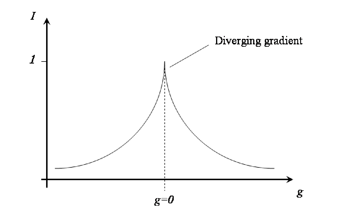
This model system has a non-standard ‘phase transition’ at $g=0$, at which some correlation functions are continuous but non-differentiable, while the ground state energy is actually analytic Wolf OVC 05. As discussed in the caption of figure (3), this behaviour is mirrored in the channel capacity.

In this section we will explore under what conditions our assumption that the regularized coherent information of equation (6):

$$Q(\{{\cal E}_{n}\}):=\lim_{n\rightarrow\infty}{I({\cal E}_{n})\over n}$$

(64)

correctly represents the true quantum capacity of our correlated channels, assuming of course that this limit exists. In the course of the discussion we will also need to consider under what conditions the regularized Holevo bound:

$$C({\cal E}_{n}):=\lim_{n\rightarrow\infty}{\chi({\cal E}_{n})\over n}$$

(65)

represents the capacity of the channel for classical information. The Holevo bound $\chi({\cal E})$ for a quantum channel ${\cal E}$ is defined as Nielsen C:

$$\chi({\cal E})=\sup_{\{p_{i},\rho_{i}\}}S({\cal E}(\sum_{i}p_{i}\rho_{i}))-\sum_{i}p_{i}S({\cal E}(\rho_{i}))$$

(66)

where the supremum is taken over all probabilistic ensembles of states $\{p_{i},\rho_{i}\}$, and $S$ as usual represents the von Neumann entropy. As pointed out in Bowen DM; Kretschmann W, showing that equations (64)/(65) are upper bounds to the quantum/classical capacity of a correlated channel is straightforward - one can use exactly the same arguments used in the memoryless case Holevo; Schumacher W; Barnum NS; Devetak. Showing that equations (64)/(65) also give lower bounds to the relevant capacities is not as simple, and may not be true for some many-body environments.

However, it turns out that if the correlations in the many-body system fall off sufficiently strongly, then the channel will be reasonably well behaved and equation (64) is true. In this section we will make this statement quantitative. We will closely follow the approach taken in Kretschmann W in the analysis of so-called forgetful channels. Some of the subtleties involved in the analysis are explained in more detail in Section VI of that paper. The conditions that we obtain are independent of the unitary which governs the interaction between each system particle and its corresponding environment, and so are applicable more widely than the dephasing interaction considered here.

References

- (1) M. A. Nielsen and I. L. Chuang, ‘Quantum Information and Computation’, Cambridge University Press 2000.
- (2) K. Banaszek, A. Dragan, W. Wasilewski and C. Radzewicz, Phys. Rev. Lett. 92 257901 (2004).
- (3) This point is discussed in detail in papers such as Kretschmann W and also in the literature on classical channels with memory (see e.g. the free online book Gray). It turns out that for all channels (not just uncorrelated ones), one may define an optimistic and a pessimistic channel capacity. In the case of channels with uncorrelated error, and in ‘well-behaved’ correlated channels, these two notions coincide, giving the conventional definition of a channel capacity.
- (4) H. Barnum, M. A. Nielsen and B. Schumacher, Phys. Rev. A 57, 4153 (1998).
- (5) G. Bowen and S. Mancini, Phys. Rev. A 69, 012306 (2004); V. Giovanetti, J. Phys. A 38 10989 (2005); N.Datta and T.C.Dorlas, J. Phys. A, 40, 8147 (2007).
- (6) D. Kretschmann and R. F. Werner, Phys. Rev. A 72, 062323 (2005).
- (7) D. Kretschmann, private communication.
- (8) G. Bowen, I. Devetak and S. Mancini, Phys. Rev. A 71, 034310 (2005).
- (9) R.M. Gray, Entropy and Information Theory, http://www-ee.stanford.edu/ gray/it.html.
- (10) I. Devetak, IEEE Trans. Inf. Th. 51, 44 (2005).
- (11) C. Macchiavello and G. M. Palma, Phys. Rev. A 65, 050301(R) (2002).
- (12) C. Macchiavello, G.M. Palma and S. Virmani, Phys. Rev. A 69, 010303R (2004).
- (13) D. Daems, Phys. Rev. A 76, 012310 (2007).
- (14) V. Karimipour and L. Memarzadeh, Phys. Rev. A 74, 032332 (2006).
- (15) E. Karpov, D. Daems and N.J. Cerf, Phys. Rev. A 74, 032320 (2006).
- (16) M.B. Plenio and S. Virmani, Phys. Rev. Lett. 99, 120504 (2007).
- (17) M. Gregoratti & R.F. Werner, J. Mod. Opt. 50, 915 (2003).
- (18) F. Buscemi, G. Chiribella and G. M. D’Ariano, Phys. Rev. Lett. 95, 090501 (2005).
- (19) F.Y. Wu, Rev. Mod. Phys. 54, 235 (1982).
- (20) M. Hamada, J. Math. Phys. 43, 4382 (2002).
- (21) A. D’Arrigo, G. Benenti and G. Falci, quant-ph/0703014.
- (22) O. Bratelli and D. Robinson ‘Operator Algebras and Quantum Statistical Mechanics’ vols. 1 & 2, Springer, (1987).
- (23) D. Welsh, ‘Codes and cryptography.’, Oxford, (1993).
- (24) Note that this does not always mean that our channel is causal in the sense discussed in Kretschmann W. As the number of qubits changes, the state of the many-body system changes, and the output of the earlier uses of the channel will change accordingly. This is in contrast to the requirement of causality imposed in Kretschmann W. However, in the limit of a large number of channel uses this effect will probably be negligible for most reasonable cases.
- (25) C.H. Bennett, D.P. DiVincenzo, J.A. Smolin, W.K. Wootters, Phys. Rev. A 54, 3824 (1996); E.M. Rains, IEEE Trans. Inf. Theo. 47, 2921 (2001).
- (26) M. D. Choi, Lin. Algebra App. 10 (3), 285-290 (1975); A. Jamiolkowski, Rep. Math. Phys 3,4 275-278 (1972).
- (27) See e.g. the lecture notes at http://www.tcm.phy.cam.ac.uk/ bds10/phase/pt.ps.gz
- (28) M. Fannes, B. Nachtergaele and R.F. Werner, Comm. Math. Phys. 144, 443 (1992).
- (29) M. M. Wolf, F. Verstraete, M. B. Hastings & J. I. Cirac, arXiv:0704.3906.
- (30) D. Pérez-García, F. Verstraete, M. M. Wolf & J. I. Cirac, quant-ph/0608197.
- (31) P. Szekeres, ‘A Course in Modern Mathematical Physics’, Cambridge (2004).
- (32) J.K. Pachos and M.B. Plenio, Phys. Rev. Lett. 93, 056402 (2004).
- (33) M.M. Wolf, G. Ortiz, F. Verstraete and J.I. Cirac, E-print arXiv cond-mat/0512180.
- (34) A. S. Holevo, IEEE Trans. Inf. Th. 44, 269 (1998).
- (35) B. Schumacher and M. Westmoreland, Phys. Rev. A 56, 131 (1997).
- (36) S. Sachdev, ‘Quantum Phase Transitions’ C.U.P. (1999).
- (37) K. Audenaert, J. Eisert, M.B. Plenio and R.F. Werner, Phys. Rev. A 66, 042327 (2002).
- (38) J. Eisert and M.B. Plenio, Int. J. Quant. Inf. 1, 479 (2003).
- (39) M.B. Plenio and S. Virmani, Quant. Inf. Comp. 7, 1 (2007).
- (40) M. Fannes, Commun, Math. Phys. 31, 291 (1973).
- (41) M. Ohya and D. Petz, Quantum Entropy and its Use, Springer, 1993
- (42) M.B. Plenio, J. Eisert, J. Dreissig and M. Cramer, Phys. Rev. Lett. 94, 060503 (2005).
- (43) M. Benzi and G.H. Golub, BIT 39, 417 (1999)
- (44) M. Cramer, J. Eisert, M.B. Plenio and J. Dreissig, Phys. Rev. A 73, 012309 (2006).
- (45) R. Bhatia, Matrix Analysis, Springer 1999.
- (46)
Bernstein’s theorem concerns the approximation
of functions by polynomials Meinardus 67.
Given the set of polynomials of degree or less with real
coefficients. For a continuous function on the interval
the best approximation error is defined as
where(122)
Now assume that is analytic in an ellipse with foci and and with half axes and . Then . Then we have Theorem (Bernstein) – Let the function be analytic in the interior of with and continuous on . In addition suppose that is real for real . Then(123)
where(124)
It is straightforward to adapt the theorem to other intervals and we will thus apply this theorem for all intervals.(125) - (47) G. Meinardus, Approximations of Functions: Theory and Numerical Methods, Springer-Verlag, New York 1967.
- (48)
Indeed we find
Lemma II (Fermions): Given two N-mode Gaussian states
characterized by fermionic covariance matrices and
fermionic symplectic eigenvalues that satisfy
then we find
where . Proof – Remember that the fermionic symplectic eigenvalues and that the entropy is given by with . Straightforward analysis shows that for and we have for all . Thus for all we find that . Inserting this into the entropy formula yields the first inequality in Lemma II. The second one follows in the same way as that of Lemma I. This completes the proof.(126)
- (49) M. Hastings, arXiv:0710.3324.