Infrared catastrophe in two-quasiparticle collision integral

1. Introduction. The ground-breaking experiments by Pothier et al. of Ref. Pothier have demonstrated that one can have a direct access to the non-equilibrium electron energy distribution function $f(E)$ and through it to the inelastic collision integral ${\cal K}_{\rm coll}(E)$ which enters the kinetic equation foot1:

In turn, studying the collision integral gives one an important information on interaction and dynamics of quasiparticles in a dirty metal. In this way the predictions of the theory of electron interaction in disordered metals AA-book; AAKh were checked Pothier; PBir and an unexpected strong sensitivity of the energy relaxation to the presence of magnetic impurities GlazKam was established.

The main idea of Ref. Pothier was to use the sharp features in the energy dependence of the density of states (DoS) $\nu_{\rm probe}(E)$ of a superconducting probe electrode, which enabled to extract $f(E)$ by measuring the differential conductance of the tunnel junction between the normal metal sample and the probe electrode. Recently, the same idea has been suggested Gia to create a non-equilibrium spin-dependent electron energy distribution $f_{\sigma}(E)$ and thereby to obtain a spin-polarized current through the probe. The sketch of the experimental setup is shown in Fig. 1. The sample in a form of a quasi-one dimensional disordered normal-metal wire is connected through the weak tunnel junctions to the two superconducting leads. The non-equilibrium is created by applying the finite bias voltage $U$ between the leads. The spin dependence of $f_{\sigma}(E)$ ($\sigma=\pm 1$ for the spin projections $\uparrow(\downarrow)$) is caused by magnetic field applied to the superconducting leads with the DoS $\nu^{(R)}_{\sigma}(E)=\nu_{S}(E+U/2\pm\sigma E_{Z})$ and $\nu^{(L)}_{\sigma}(E)=\nu_{S}(E-U/2+\sigma E_{Z})$ where $\nu_{S}(E)=\nu\,\Re\left[E/\sqrt{E^{2}-\Delta^{2}}\right]$ and the Zeeman shift $E_{Z}=\mu_{B}H$ is taken with the sign $\pm$ depending on whether the directions of the magnetic field in the right and left leads are parallel or anti-parallel. In the absence of relaxation $f_{\sigma}(E)$ is given by Gia; Klap:

where $f_{F}(E)$ is the Fermi distribution function. The measured quantity is the differential conductance with respect to the probe bias $V_{\rm probe}$ across the probe tunnel contact. The probe contact can act as a spin-analyzer provided an additional magnetic field is also applied to a superconducting probe electrode.

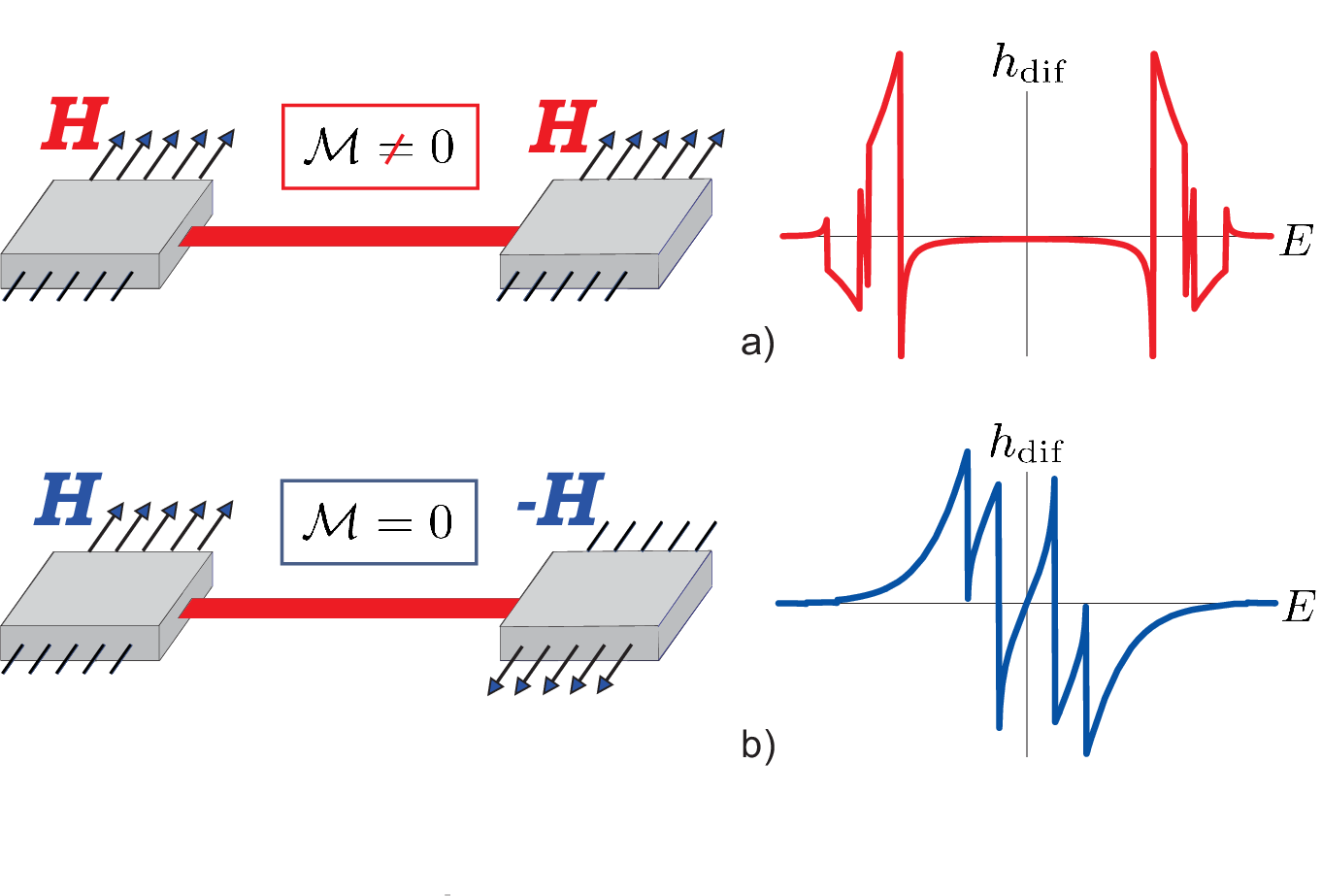
There are two distinct cases schematically shown in Fig. 2a and Fig. 2b: (i) with parallel and (ii) with anti-parallel magnetic fields in the superconducting leads. In the former case a non-equilibrium state with a nonzero total spin polarization

is created, while in the latter case ${\cal M}=0$. The typical form of the difference $f_{\rm dif}=f_{\uparrow}(E)-f_{\downarrow}(E)$ that follows from Eq. (2) is shown in Fig. 2 in both cases.

The aim of this work is to consider the relaxation of such a spin-dependent distribution caused by the electron-electron interaction. For this we derive the collision integral ${\cal K}_{\rm coll}$ in the approximation of the two-quasiparticle collisions in the case where both the spin-singlet and the spin-triplet channel of the interaction are present. The detailed derivation of the collision integral due to the electron-electron interaction has been recently carried out in Refs. AhCatAl; CatAl. However, the analysis has been limited to the case of the spin-independent distribution functions $f(E)$, while we are going to focus on the relaxation of the difference $f_{\rm dif}(E)$. The results of calculation of the collision integral for the spin-dependent distribution function have been also recently reported in Ref. Schel-Bur. However, the authors considered a limited class of distributions with a very particular spin-dependence equivalent to a shift in the energy $f_{\uparrow}(E)=f_{\downarrow}(E+\delta E)$. Such type of dependence does not hold e.g. in the experimental setup of Figs. 1, 2.

The main qualitative result of our analysis is that there are three different contributions in the collision integral. Two of them are also present if only the singlet channel of the interaction is considered, with only their amplitudes depending on the triplet channel interaction constant $F$. The third contribution corresponding to the spin-flip process is only present when the triplet channel of the interaction is taken into account. Its magnitude depends Schel-Bur essentially on the conserving total spin ${\cal M}$. However more importantly, it is singular for the non-equilibrium spin-dependent distribution with ${\cal M}=0$ which naturally arises in the experimental situation (ii) of Fig. 2b. The existence of such a singularity which never occurs if only the singlet channel of the interaction is present, is the main qualitative result of this work.

2.Three contributions to the collision integral. For a generic two-quasiparticle collision in a disordered metal in the absence of spin-orbit interaction and magnetic impurities two quantities are conserved: the total energy ${\cal E}$ and the total spin ${\cal M}$. The latter conservation law allows only three possible processes (see Fig. 3): (i) in the initial state the quasiparticles have the same spin projections $(1/2)\sigma$ which remain unchanged during the collision, (ii) in the initial state the quasiparticles have opposite spin projections which do not change during the collision, (iii) in the initial state the quasiparticles have opposite spin projections and the collision results in a spin-flip of both quasiparticles. Each process corresponds to a certain term in the collision integral that contains combinations of the type $f^{\rm in}(E+\omega)\,f^{\rm in^{\prime}}(E^{\prime})\,[1-f^{\rm fin}(E)]\,[1-f^{\rm fin^{\prime}}(E^{\prime}+\omega)]-[1-f^{\rm in}(E+\omega)]\,[1-f^{\rm in^{\prime}}(E^{\prime})]\,f^{\rm fin}(E)\,f^{\rm fin^{\prime}}(E^{\prime}+\omega)$ which for the processes (i)-(iii) take, respectively, the forms:

where $h_{\sigma,E}=1-2f_{\sigma}(E)$.

The collision integral ${\cal K}_{\rm coll}(\sigma,E)$ can be represented as follows:

where $\nu$ is the DOS (per spin direction) of the normal-metal sample at the Fermi level. The quantities $K_{p}^{\sigma}(\omega)$ describe the strength of relaxation due to the corresponding processes (the quantities corresponding to the singlet channel $K_{1,2}^{\sigma}(\omega)=K_{1,2}(\omega)$ does not depend on ${\cal M}$ and hence on $\sigma$). We obtained the following expressions for them valid in the limit $p_{F}\ell\gg 1$ ($p_{F}$ is the Fermi momentum, $\ell$ is the elastic scattering length) and for the diffusive quasiparticle dynamics:

In Eqs. (8)-(Infrared catastrophe in two-quasiparticle collision integral) by $F$ ($F=-1$ corresponds to the Stoner instability) we denoted the Fermi-liquid constant corresponding to the triplet channel of the electron-electron interaction. The summation over ${\bf q}$ can be replaced by integration $\frac{1}{{\cal V}}\sum_{q}\rightarrow\int\frac{d^{d}q}{(2\pi)^{d}}$ in the limit $\omega\gg E_{Th}\equiv D/L^{2}$ ($D$ is the diffusion coefficient, $L$ is the length of the disordered sample) which will be considered below.

Note that at small $F\ll 1$ we obtain up to the linear in $F$ terms: $K_{3}=0$ and

In this limit the spin-spin interaction in the triplet channel results in only a small (and opposite in sign for the parallel and anti-parallel spins of the two quasiparticles in the initial state) change in the amplitudes of the processes (i) and (ii) which are dominated by the singlet channel of the electron-electron interaction. Note that under the restrictions on the form of the spin-dependence of $h_{\sigma,E}$ adopted in Ref. Schel-Bur the combinations $I^{(1)}_{\sigma}$ and $I^{(2)}_{\sigma}$ appeared to be identical. This is why the result of Ref. Schel-Bur contained only the combination $(K_{1}+K_{2})I^{(1)}_{\sigma}$ and $K_{3}^{\sigma}I^{(3)}_{\sigma}$.

3. Relaxation of a non-equilibrium distribution and the conservation laws. As has been already mentioned, the form of the collision integral should be compatible with the two conservation laws. The conservation of the total energy requires:

The conservation of the total spin polarization leads to:

One can check using Eqs. (4)-(Infrared catastrophe in two-quasiparticle collision integral) that fulfillment of those two conservation laws is guaranteed by the structure of $I^{(p)}_{\sigma}(E,\omega)$ and the following properties of the kernels $K_{p}(\omega)$:

What we would like to note here is that the full relaxation to equilibrium due to the electron-electron interaction is only possible if ${\cal M}=0$. Indeed, the fixed solutions to the kinetic equation Eq. (1) which correspond to all combinations Eq. (4)-(6) vanishing identically, are the Fermi distribution functions $f_{\uparrow(\downarrow)}^{(0)}(E)=f_{F}(E\mp{\cal M}/2)$. Any non-equilibrium distribution tends to relax to these fixed solutions. However only at ${\cal M}=0$ we have $f_{\uparrow}^{(0)}(E)\equiv f_{\downarrow}^{(0)}(E)$ which corresponds to the complete equilibrium. So we encounter for the first time with the special role of the ${\cal M}=0$ condition.

4. Collision integral for a quasi-1d wire and the infrared catastrophe at ${\cal M}=0$. For the quasi-1d experimental geometry of Fig. 1, Eqs. (8)-(Infrared catastrophe in two-quasiparticle collision integral) can be straightforwardly evaluated:

where $S$ is the cross-section area of the quasi-1d wire,

$C_{2}=1$, $C_{3}=F^{2}/2$ and the legitimate values of $F$ are $F>-1$.

A remarkable property Schel-Bur of $K_{3}^{\sigma}$ is that it depends on the spin polarization ${\cal M}$. For ${\cal M}\neq 0$ $K_{3}^{\sigma}(\omega)$ is finite at all values of $\omega$ and the collision integral is well defined. A peculiar situation arises when ${\cal M}=0$. In this case $K_{3}^{\sigma}(\omega)\propto\frac{1}{|\omega|^{3/2}}$ is singular at $\omega=0$. At the first glance there is nothing special in such a degeneracy which is the same as for the standard case of the electron-electron interaction in the singlet channel Pothier; AA-book. The difference, however, is in the form of $I^{(3)}_{\sigma}$ as compared to $I^{(1,2)}_{\sigma}$. As is seen from Eqs. (4)-(6), the cancellations of the “in” and “out” terms lead to: $I^{(1,2)}_{\sigma}(\omega=0)=0$ for any $f_{\sigma}(E)$, while $I^{(3)}_{\sigma}(\omega=0)\neq 0$ unless $f_{\rm dif}=f_{\uparrow}(E)-f_{\downarrow}(E)$ is identically zero. This means that the singularity $K_{p}(\omega)\propto\frac{1}{|\omega|^{3/2}}$ is not dangerous for terms proportional to $I^{(1,2)}_{\sigma}$ (which are the only terms that arise in the case of electron-electron interaction in the singlet channel) but it leads to the divergency of the term $\propto I^{(3)}_{\sigma}$ corresponding to the spin-flip processes due to the electron-electron interaction in the triplet channel. So we have an infrared catastrophe in the collision integral in the case of a spin-dependent electron energy distribution with ${\cal M}=0$.

5. Derivation of the collision integral. Before we discuss the physical origin of such a catastrophe and the ways to cure it we briefly outline the derivation of the collision integral Eqs. (4)-(6),(8)-(Infrared catastrophe in two-quasiparticle collision integral).

Following the original work of Keldysh Keldysh we represent the collision integral as follows:

where

and $\Sigma^{R,A,K}$ and ${\cal G}^{R,A,K}$ are retarded, advanced and Keldysh components of the self-energy part and an exact single-particle Green’s function. In the two-quasiparticle collision approximation we adopt in this paper, the self-energy part is given by:

where the integration over $\omega$ and a proper summation over spin indices $\alpha,\beta,\gamma,\delta$ is assumed in all three equations.

In this approximation we neglect (a) the interaction corrections to the vertex part $\Gamma=1$ and (b) the interaction corrections to the single-particle Green’s function ${\cal G}_{E+\omega}$ which is supposed to be equal to the corresponding Green’s function without interaction $G_{E+\omega}$. In Eqs. (24) we denote by ${\cal D}_{\omega}$ the dynamically screened interaction:

where $\hat{\sigma}^{i}$ ($i=1,2,3$) are the Pauli matrices $\hat{\sigma}_{x,y,z}$ and $\hat{\sigma}^{4}$ is the unit matrix.

The $4\times 4$ interaction matrix $D^{R(A)}_{ij}$ obeys an RPA-like equation:

where $U_{i}$ ($i=1,2,3$) is the bare interaction constant $F^{\sigma}=F/(4\nu)$ of the electron-electron interaction in the triplet channel:

and $U_{4}\equiv U^{\rho}=F^{\rho}+V(q)$ is the bare interaction in the singlet channel which at small $q$ is dominated by the Coulomb interaction $V(q)\rightarrow\infty$:

The generalized polarization bubbles are given by

where the retarded and advanced polarization bubbles $\pi^{R(A)}_{\alpha\beta}\rightarrow G^{R(A)}_{\alpha\alpha}G^{K}_{\beta\beta}+G^{K}_{\alpha\alpha}G^{A(R)}_{\beta\beta}$ for the spin-independent single particle Hamiltonian (no magnetic impurities and no spin-orbit interaction) contain retarded, advanced and Keldysh Green’s functions.

The Keldysh component $D^{K}_{ij}$ of the dynamically screened interaction is expressed explicitly through $D^{R}_{ij}$ and $D^{A}_{ij}$:

where $\Pi^{K}_{ij}$ is given by Eq. (31) but with $\pi^{K}_{\alpha\beta}\rightarrow G^{K}_{\alpha\alpha}G^{K}_{\beta\beta}+G^{R}_{\alpha\alpha}G^{A}_{\beta\beta}+G^{A}_{\alpha\alpha}G^{R}_{\beta\beta}$.

The central point of the derivation of the collision integral is the ansatz that involves the non-equilibrium electron energy distribution function $h_{\sigma,E}$:

The similar ansatz has been suggested by Keldysh Keldysh for the exact Green’s functions. We will be using Eq. (33) for the Green’s functions without electron-electron interaction. The reason is that the perturbation theory in interaction can be built using Eq. (33) with an arbitrary “initial” distribution function $h^{(0)}_{\sigma,E}$ compatible with the Fermi statistics. It will cancel out anyway in the final result as the initial distribution has to be forgotten in the non-equilibrium steady state. Diagrammatically this cancellation happens because of the proliferation of singular “loose diffusons” KY which, however, make impossible the perturbative analysis. There is only one single choice of $h^{(0)}_{\sigma,E}$ in Eq. (33) – the true solution $h_{\sigma,E}$ of the kinetic equation – when such proliferation does not occur and all the diagrams with loose diffusons are equal to zero KY.

Using Eq. (33) one can obtain the following expressions for the polarization bubbles:

where $\Delta G_{E}=(G^{R}-G^{A})_{E}$ and an integration over $\int dE^{\prime}/2\pi$ is assumed. The next step is the standard disorder average of the product $G^{R}_{E^{\prime}+\omega}G^{A}_{E^{\prime}}$ with the result

This eliminates the dependence on $E^{\prime}$ everywhere but in the distribution functions $h_{\alpha,E^{\prime}}$.

At this point it is appropriate to note on the difference between $\pi^{R(A)}_{\alpha\alpha}$ (or the spin-independent case) and $\pi^{R(A)}_{\alpha\beta}$ with $\alpha\neq\beta$. In the former case one can use an identity

which holds for an arbitrary function $h_{\alpha,E^{\prime}}$ which at $|E^{\prime}|\rightarrow\infty$ converges sufficiently fast to $\mathrm{sign}(E^{\prime})$. Then one immediately obtains the standard result which is independent of the electron energy distribution function:

In contrast to that, the corresponding integral in $\pi^{R}_{\alpha,-\alpha}$ contains a part $\int dE^{\prime}\,(h_{\alpha,E^{\prime}}-h_{-\alpha,E^{\prime}})$ proportional to the total spin polarization ${\cal M}$ of the non-equilibrium state given by Eq. (3). Thus we obtain:

where the sign $\mp$ corresponds to $\alpha=\uparrow(\downarrow)$. For completeness we also give an expression for $\pi^{K}_{\alpha\beta}$:

The dependence of Eqs. (40),(41) on the spin projections $\alpha,\beta$ makes the $4\times 4$ matrices $\Pi^{R,A,K}_{kl}$ non-diagonal:

where for any of the omitted superscripts $R,A,K$

Correspondingly, the $4\times 4$ matrices $D^{R,A,K}_{ij}$ found from Eqs. (28),(32) appear to have the off-diagonal structure similar to Eq. (Infrared catastrophe in two-quasiparticle collision integral). For $D^{R(A)}=(1-U\Pi^{R(A)})^{-1}U$ we obtain:

with

Respectively, for $D^{K}$ we have:

In Eqs. (53),(Infrared catastrophe in two-quasiparticle collision integral) we took the limit $U^{\rho}\rightarrow\infty$ that corresponds to $|V({\bf q})\pi^{R(A)}(\omega,{\bf q})|\gg 1$ which is always the case at small enough $|{\bf q}|$, as $V({\bf q}\rightarrow 0)$ diverges because of the long-range character of Coulomb interaction.

Substituting Eqs. (24)-(Infrared catastrophe in two-quasiparticle collision integral) into Eq. (18), neglecting interaction correction to the Green’s function ${\cal G}_{E}\approx G_{E}$ and using Eq. (37) for the disorder average of still not averaged pair of Green’s functions we arrive at the main quantitative result of this paper given by Eq. (4)-(Infrared catastrophe in two-quasiparticle collision integral).

6. Conclusion. We have shown above that the relaxation of the spin-dependent electron energy distribution at the total spin magnetization ${\cal M}=0$ differs qualitatively from the case ${\cal M}\neq 0$. It is only in this case that the complete relaxation to a spin-independent Fermi distribution is possible due to electron-electron interaction alone. And it is in this case that the infrared catastrophe is encountered in the collision integral for a quasi-1d disordered wire. As a result, an anomalously fast relaxation to a spin-independent non-equilibrium distribution happens well before the complete equilibrium is reached. The corresponding collision integral responsible for such a fast relaxation can be approximated as

where

with $C(F)=\frac{F^{2}}{(1+\sqrt{1+F})(2+F)\sqrt{1+F}}$.

A remarkable feature of Eq. (57) emerging due to the infrared catastrophe is the quasi-elastic form of the collision integral. If the infrared cut-off $1/\tau_{0}$ in the divergent integral $\int_{1/\tau_{0}}\frac{d\omega}{|\omega|^{3/2}}$ is small compared to the effective temperature, one can set $\omega=0$ in the distribution functions $f_{\sigma}$ entering Eq. (6). Thus we arrive at Eq. (56) which dependence on $f_{\sigma}(E)$ is identical to the elastic part of the collision integral due to magnetic impurities. The only difference is that the coefficient $K_{\sigma}$ also depends on the integral of the distribution functions. Thus the triplet part of the electron-electron interaction acts in this case similar to the magnetic impurities.

References

- (1) H. Pothier, S.Gueron, N. O. Birge, D. Esteve, and M. H. Devoret, Phys. Rev. Lett. 79, 3490 (1997).
- (2) Here and below we assume the case of dirty metal where the distribution function depends only on energy and (slowly) on the space and time coordinates .
- (3) B. L. Altshuler and A. G. Aronov, in Electron-Electron Interactions in Disordered Systems , edited by A. L. Efros and M. Pollak (Elsevier, New York, 1985)
- (4) B. L. Altshuler, A. G. Aronov and D. E. Khmelnitskii, J. Phys. C. 15, 7367 (1982).
- (5) F. Pierre, A. B. Gougam, A. Anthore et al., Phys. Rev. B. 68, 085413 (2003).
- (6) A. Kaminski and L. I. Glazman, Phys. Rev. Lett. 86, 2400 (2001).
- (7) F. Giazotto, F.Taddei, R. Fazio and F. Beltram, Phys. Rev. Lett. 95, 066804 (2005).
- (8) Y. Ahmadian, G. Catelani and I. L. Aleiner, Phys. Rev. B. 72, 245315 (2005).
- (9) G. Catelani and I. L. Aleiner, JETP 100, 331 (2005).
- (10) N. M. Chtchelkatchev and I. S. Burmistrov, arXiv: 0708.0523.
- (11) D. R. Heslinga and T. M. Klapwijk, Phys. Rev. B 47, 5157(1993).
- (12) L. V. Keldysh, Zh. Eksp. Teor. Fiz. 47, 515 (1964) [Sov. Phys. JETP 20, 1018 (1965)].
- (13) V. I. Yudson and V.E.Kravtsov, Phys. Rev. B. 67, 155310 (2003); V. I. Yudson E. Kanzieper and V.E.Kravtsov, Phys. Rev. B. 64, 045310 (2001);