Supplementary Information for “A black hole in an eclipsing binary in the nearby spiral galaxy Messier 33”
Department of Astronomy, San Diego State University, 5500 Campanile Drive, San Diego, CA 92182-1221, USA.
Harvard-Smithsonian Center for Astrophysics, 60 Garden Street, Cambridge, MA 02138, USA.
Department of Astronomy, Yale University, PO Box 208101, New Haven, CT 06520-8101, USA.
National Optical Astronomy Observatory, 950 North Cherry Avenue, Tuscon, AZ 85719, USA.
Max-Planck-Institut für extraterrestrische Physik, Giessenbachstraße, D-85741 Garching, Germany.
MIT Kavli Institute for Astrophysics and Space Research, 77 Massachusetts Avenue, 37-287, Cambridge, MA 02139, USA.
Wise Observatory, Tel Aviv University, Tel Aviv 69978, Israel.
This Supplementary Information provides details about the spectral extraction (crowding issues and the removal of nebular lines), a discussion about the distance to M33, a model for the O-star wind and the measurement of the true photospheric X-ray eclipse width , and details about ellipsoidal modelling. It also contains five related figures, one related table, and additional references.
1 Supplementary methods
1.1 Crowding issues:
M33 X-7 lies in a moderately crowded OB association known as HS 13 (ref. 23). Fortunately, HS 13 has been observed using the Hubble Space Telescope and the WFPC2. In ref. 5 it is shown that apart from a close pair (0.2 arcsecond separation) of stars 0.9 arcseconds to the southwest, the optical counterpart of M33 X-7 is relatively isolated. For the spectroscopic observations from the Gemini-North Telescope, the 0.5 arcsecond wide slit was placed at a position angle of 215.6 degrees, which is the angle defined by M33 X-7 and the close pair of neighbour stars, which are the only potential source of contamination.
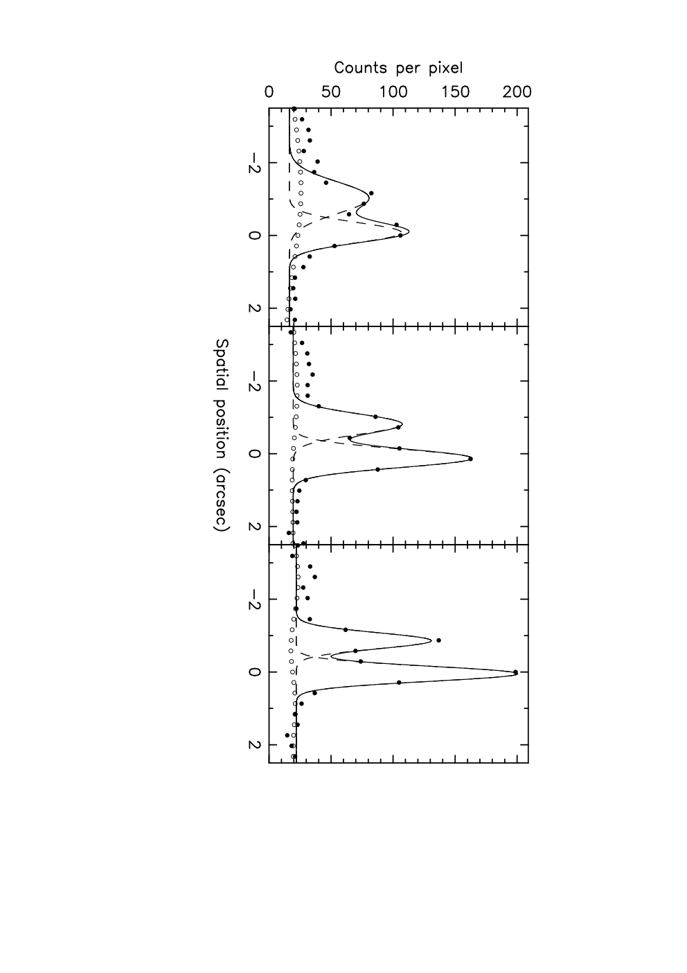
The detector in the GMOS instrument consists of three EEV CCD chips in a row with mm gaps in between. The dispersion axis runs along the longer dimension of the mosaic. Supplementary Figure 1 shows spatial profiles of M33 X-7 and the neighbour stars near H for three observations that represent relatively “poor” seeing (about 0.8 arcseconds), “average seeing” (about 0.6 arcseconds), and “good” seeing (about 0.4 arcseconds). The majority of the spectra were similar to the “average” case. Gaussian fits to the spatial profiles and simple numerical integration show that the area in the overlap region of the two profiles is typically 5-10% and at most 20% of the area under the M33 X-7 profile. For the spectral extraction with the GMOS pipeline, the lower extraction aperture was placed slightly to the right of the “dip” between the two profiles, which was sufficient to exclude light from the neighbour stars.
1.2 Removing nebular lines:
As noted above, M33 X-7 lies in an OB association, and light from the surrounding HII region is evident in both the direct images and in the two-dimensional spectra. Unfortunately, the background nebular light varies over small spatial scales and is not removed by the regular GMOS spectral extraction routines, which assume that the background light is uniform over the entire spatial extent of the two-dimensional spectra. Also, the presence of the close pair of neighbour stars makes it harder to use higher order polynomials when fitting the background region.
The SPECRES package in IRAF provides tools to extract point source spectra with complex backgrounds22. The spatial profile of a point source is distinguished from the quite different profile of an extended background source using a Gaussian smoothing kernel along with a Richardson-Lucy type of iterative restoration algorithm that performs a maximum likelihood estimation. For optimal results, one must precisely specify the positions of the point sources, the variation of the spatial position of the point sources with wavelength, and the spatial “Slit Spread Function” (SSF) with wavelength. A list of the relative positions of the point sources along the slit was made from the Gemini direct images and also the archival HST images. Given the list of relative positions, the positions of the sources on a given observation can be found once the position of a reference source is measured. The variation of the position of the spectra with wavelength (the “slope”) is easily measured using the extraction tools in the GMOS package. Unfortunately, the derivation of the SSF is somewhat more involved since it depends on the properties of the instrument and on the observing conditions. The “specpsf” task in SPECRES was employed to make SSFs from the direct images that were taken immediately following each spectroscopic observation and by using analytic functions (Gaussians and Lorentzians) with widths that varied with wavelength.
Once the point source positions, the slope, and SSFs are determined, one must decide on a width for the smoothing kernel that is used to distinguish between point sources and extended background sources. There is a trade-off between the width of the kernel and the signal-to-noise (SN) in the extracted spectra. A broad smoothing kernel will result in spectra with higher SN, but the background subtraction will be poor if the background varies on small spatial scales. On the other hand, a narrow smoothing kernel will result in spectra with good background subtraction, but at the expense of lower SN in the extracted spectrum.
Since the observing conditions change from observation to observation, the optimal set of parameters for one spectrum may not be appropriate for another spectrum. To optimise the spectral extraction for each observation, we wrote scripts that performed the spectral extraction with a wide range of variations of the position of the reference source, the spectral slope, the variation of the width of the SSF with wavelength, and the size of the smoothing kernel. For each observation, 372 extractions were performed, and the optimal extraction was determined by cross correlation with a synthetic spectrum as the template.
With the exception of the stronger [O III] line and H, the nebular lines were cleanly removed in all of the spectra. Supplementary Figure 2 shows a spectrum extracted with the GMOS pipeline software and the spectrum extracted with SPECRES. The nebular lines are mostly gone in the latter spectrum, although note the higher noise level.
Since the H emission line was never cleanly removed, we excluded this feature when modelling the spectrum and computing the radial velocities. As a check on the results, we note that the radial velocity curve derived from the SPECRES extracted spectra (using several Balmer lines and He I lines in the cross correlation region 4000-4375 and 4450-4565 Å) is virtually the same as the radial velocity curve derived from the GMOS pipeline extracted spectra (using the two strong He II lines noted in the main text). For example, for the former, we find km s-1 and for the latter we find , which are in close agreement with our adopted value in Table 2, main text.
1.3 The distance to M33:
We estimate the distance to M33 using four indicators. Because of the differential nature of distance measurements, we express our intermediate results as relative distance moduli with respect to the Large Magellanic Cloud (LMC), and then place the final result on an absolute scale.
Tip of the Red Giant Branch: Tip of the red giant branch (TRGB) magnitudes for ten fields in M33 are given in ref. 26, and a global TRGB value for the LMC is derived in ref. 27. Both measurements were carried out using the same calibration of the technique, which includes a small ( mag) metalicity correction. We find mag.
Cepheids: and photometry of 61 Cepheids in M33 with periods from 15 to 80 days is presented in ref. 28, which were fitted with LMC period-luminosity (P-L) relations from the OGLE project[29]. We apply an updated correction for the metalicity dependence of the Cepheid P-L relation, based on the results in refs. 30 and 31, that amounts to mag. Thus, we obtain mag.
RR Lyrae: Sixty four RR Lyrae variables in M33 discussed in ref. 32 were used to derive an average extinction-corrected magnitude for the sample of mag. New photometry and spectroscopy for over 100 objects in the bar of the LMC is presented in ref. 33, from which an average value of mag was derived. While these values are already corrected for the metalicity dependence of the RR Lyrae, the calibrations used by the authors are slightly different (e.g. ref. 34 vs. ref. 35). This results in an additional mag correction to the results in ref. 32, bringing the relative distance modulus to mag.
Red Clump: An extinction-corrected -band magnitude of the red clump in the LMC of mag is given in ref. 33. An equivalent value for M33 of mag was determined in ref. 26. Both references use two sets of calibrations for the red clump magnitude as a function of metalicity[36, 37] which results in a small ( mag) metalicity correction and a relative distance modulus of mag.
The average distance modulus of these four techniques, weighted by their uncertainties, is mag.
We calculate the true distance modulus of the LMC based on the weighted average of three recent and independent estimates. First, the study of several detached eclipsing binary systems (DEBs)[38] yields an LMC distance modulus of mag. Second, parallaxes of Galactic Cepheids obtained with the Hubble Space Telescope yield an absolute calibration of the Cepheid P-L relation that, when applied to the LMC, gives a distance modulus of mag (after a correction for metalicity dependence). Lastly, the relative Cepheid distance modulus between NGC 4258 and the LMC[30], coupled with the maser distance to the former[39], gives mag. The average of these values (weighted by their uncertainties) is mag.
In conclusion, the combination of and yields mag, which corresponds to a distance of kpc.
We note that our result is in disagreement with the recent distance determination to M33 in ref. 40, who obtain mag, or kpc based on a DEB. This is a puzzling result, because it implies a relative distance modulus between the LMC and M33 based on DEBs of mag. The DEB technique has been applied to a similar system in M31 (ref. 41) and in that case, the relative distance modulus between M31 and the LMC is in excellent agreement with other methods.
1.4 Modelling the O-star wind and measuring the photospheric X-ray eclipse width in M33 X-7:
The mean X-ray luminosity of M33 X-7 is erg s-1. For an inclination of , and using a limb darkening law[42] given by , the isotropic luminosity is erg s-1. For a nominal 10% accretion efficiency, this corresponds to a mass accretion rate of g s yr-1. We use this estimate to constrain the O-star wind.
The X-ray intensity following egress increases steeply by roughly a factor of 15 ( counts s-1 versus counts s-1; Supplementary Figure 3). Using the out-of-eclipse spectral models in ref. 5 and a metalicity of 10% of the solar value, the column density of gas required to attenuate the X-ray flux by a factor of 15 is g cm-2.
As a function of radius , the velocity of a radiatively driven O-star wind has a profile of the form[43]
| (1) |
where is the asymptotic speed of the wind at large radius, is the radius of the O-star, and is an index which typically has a value in the range 0.8 to 1.2. In the following, we take km s-1, a typical value for O-stars, , and the value of given in Table 2 (main text): cm. With cm (Table 2, main text), the wind velocity at the radius corresponding to the location of the black hole () is then km s-1.
The mass accretion rate onto the black hole may be roughly estimated via the Bondi-Hoyle formula (e.g. ref. 44),
| (2) |
where is the density of the wind at . This formula is only approximately correct and we should include an unknown coefficient to allow for uncertainties. However, numerical simulations[45] show that the coefficient is not very different from unity.
Equating the expression for in equation (2) to the previously estimated mass accretion rate of g s-1, we find g cm-3. The mass loss rate in the O-star wind is then
| (3) |
For comparison, the mass loss rate derived from line-force computations[46] is (), assuming an O-star luminosity and mass given in Table 2 (main text), a temperature between 34,000 and 36,000 K, a metalicity between 0.1 and 0.3 times the solar value, and . This mass loss rate is a factor of 5 smaller than the value we derived. However, the plots that compare the predicted mass loss rates with observed values for LMC and SMC stars (Figs. 6 and 7 in ref. 46) have a scatter of up to 0.6 dex (e.g. nearly a factor of 4). We therefore do not consider the difference between the mass loss rate we derived and the one derived from the line-force computations significant. Finally, using , the wind density at radius is
| (4) |
We have assumed a spherically symmetric wind, which is perhaps not a very good approximation[47], but it is hard to know how to improve on this.
The photosphere of the O-star is located at a radius such that the radial column density from infinity down to is equal to g cm-2, which is the column depth to the surface in the best-fitting model atmosphere:
| (5) |
Solving, we find that is extremely close to the O-star radius of . Thus, the presence of the wind has a negligible effect on the radius of the photosphere.
The X-ray eclipse light curve, however, is strongly affected by the wind. Let us define the critical radius of the eclipse to be the impact parameter at which the line-of-sight column density is equal to 0.7 g cm-2. Thus
| (6) |
where gives the position of the X-ray source. Solving this condition numerically, we obtain an eclipse width of .
There are uncertainties in many of the parameters we have used. Let us allow for all the uncertainties by varying by a factor of 1.5 either way around the estimate in equation (3). Over this entire range of , continues to remain very close to , so the wind has no effect on the photosphere. At the lower end of the range, we obtain for the eclipse radius , while at the upper end, we find . The observed width of is bracketed by these values.
According to this model, the photosphere subtends an angle of in the light curve, while the eclipse, which is defined by the positions at which the X-ray flux falls by a factor of 15, subtends an angle in the range . Thus, the ratio of the eclipse angle to the photospheric angle lies in the range 1.06 to 1.19. Turning this around, since the observed eclipse angle is , we estimate the photospheric angle to lie in the range .
The X-ray light curve itself suggests an angle close to (Supplementary Figure 3). We fitted two line segments to the ACIS count rate data and found that the transition from the flat bottom to egress occurs between ( and (, depending on how the data are binned and how they are fitted (i.e., versus median fitting). Thus, in modelling the binary system, we set (Table 2, main text). Although we are confident that is the appropriate value to use, we nevertheless show below that derived geometrical parameters change only modestly for values of between and .
1.5 Modelling and error estimation:
We used the statistic to evaluate the goodness-of-fit between the observed light and velocity curves and their model counterparts:
| (7) | |||||
| (8) |
Here, the notation are the observed , , , and magnitudes at orbital phase , respectively, is the uncertainty on the measurement at , and is the model value at . We also have three observed quantities that constrain the available parameter space, namely the duration of the X-ray eclipse , the radius of the secondary star , and the projected rotational velocity of the secondary star . For each model that is computed, these three quantities can be determined. Hence, there are three additional contributions to :
| (9) | |||||
| (10) | |||||
| (11) |
Our total is then
| (12) |
In any optimisation procedure, there is always the issue of assigning relative weights to different data sets. After our extensive initial searches of parameter space resulted in a good solution, we scaled the uncertainties on each data set (e.g., four light curves and one radial velocity curve) so that the total of the fit was equal to for each data set separately. The required scalings and number of observations for each data set were 0.8715 for 30 observations in , 0.9505 for 70 observations in , 1.0064 for 39 observations in , 1.0449 for 24 observations in , and 0.9452 for 22 radial velocity observations. After the scaling, the optimiser codes were run again to produce the final set of parameters. The resultant of the best-fitting solution is .
We computed the confidence limits of the fitted and derived parameters using a brute force method. When a model was computed, we saved the value of fitted parameters, the derived parameters (e.g., the mass of the compact object, surface gravity of the companion, etc.), and the of the fit. After a suitably large number of runs of the genetic optimiser and the grid search optimiser, we computed models and values almost everywhere near the global minimum in the 10-dimensional parameter space. It was then a simple matter to project one dimension of the hypersurface along any parameter of interest. Supplementary Figure 4 shows vs. parameter value for twelve fitted and derived parameters. A sixth order polynomial was fitted to each curve to determine the value of the parameter at the minimum , and to compute the formal 1, 2, and confidence intervals (taken to be the range in the parameter needed to make , , and , respectively). Each of the parameters shown in the figure are well determined, since the curves have smooth shapes with clear minima. The non-zero eccentricity is significant at about the level, as is the indication of non-synchronous rotation (e.g. the parameter is different than 1.0 by ). On the other hand, models with no accretion disk are ruled out at the level of several since the best-fitting model with no accretion disk has a of more than 210.
As a check, extensive fits were made assuming different values of the X-ray eclipse width . Supplementary Table 1 shows the best-fitting values of the inclination, secondary star mass, black hole mass, and for various assumed values of . Over the whole range of (), the inclination changes from to , and the black hole mass only changes from to .
1.6 Comparison of ellipsoidal model with additional light curves:
Supplementary Figure 5 shows all of the available optical light curves of M33 X-7 phased on the X-ray ephemeris5: and light curves from the DIRECT survey (see ref. 10), and from the Gemini North Telescope, and from the Canada-France-Hawaii Telescope (CFHT) M33 Variability Survey (see ref. 11) and , , and from WIYN. The CFHT and WIYN light curves have anomolously faint points near phase 0 (1.e., near X-ray eclipse) that we cannot explain (there are no obvious defects in the images in question). These same light curves also have deeper minima near phase 0.5 (when the X-ray source is in front of the O-star companion), which, unlike the low points near phase 0, can easily be explained qualitatively by increasing the radius of the accretion disk from 45% of the black hole’s Roche lobe radius to . The out-of-eclipse X-ray flux of M33 X-7 is variable, so an accretion disk with a changing radius is perhaps not unexpected. Alternatively, if the plane of the accretion disk is not exactly parallel to the plane of the binary orbit, and the disk precesses, then its cross sectional area on the plane of the sky would change. This would result in changes in the depth of the light curve minimum near phase 0.5.
We note that in the DIRECT, Gemini, and CFHT light curves the maximum near phase 0.75 is consistently higher than the maximum near phase 0.25. The small orbital eccentricity in our model explains the slight difference between the heights of the maxima.
2 Supplementary notes
References
- [26] Kim, M., Kim. E., Lee, M. G., Sarajedini, A. & Geisler, D. Determination of the distance to M33 based on the tip of the red giant branch and the red clump. Astron. J. 123, 244-254 (2002).
- [27] Sakai, S., Zaritsky, D., & Kennicutt, J. C. The tip of the red giant branch distance to the Large Magellanic Cloud. Astron. J. 119, 1197-1204 (2000).
- [28] Macri, L. Ph.D. Thesis, Harvard University (2001).
- [29] Udalski, A., Szymanski, M., Kubiak, M., Pietrzynski, G., Soszynski, I., Wozniak, P. & Zebrun, K. The Optical Gravitational Lensing Experiment. Cepheids in the Magellanic Clouds. III. period-luminosity-color and period-luminosity relations of classical Cepheids. Ac. A. 49, 201-221 (1999).
- [30] Macri, L. M., Stanek, K. Z., Bersier, D., Greenhill, L. J. & Reid, M. J. A new Cepheid distance to the maser-host galaxy NGC 4258 and its implications for the Hubble constant. Astrophys. J. 652, 1133-1149 (2006).
- [31] Sakai, S., Ferrarese, L., Kennicutt, R. C. & Saha, A. The effect of metallicity on Cepheid-based distances Astrophys. J. 608, 42-61 (2004).
- [32] Sarajedini, A., Barker, M. K., Geisler, D., Harding, P. & Schommer, R. RR Lyrae variables in M33. I. Evidence for a field halo population. Astron. J. 132 1361-1371 (2006).
- [33] Clementini, G., Gratton, R., Bragaglia, A., Carretta, E., Di Fabrizio, L. & Maio, M. Distance to the Large Magellanic Cloud: The RR Lyrae stars. Astron. J. 125 1309-1329 (2003).
- [34] Chaboyer, B., Green, E. M. & Liebert, J. The age, extinction, and distance of the old, metal-rich open cluster NGC 6791. Astron. J. 117, 1360-1374.
- [35] Gratton, R. G., Bragaglia, A., Carretta, E., Clementini, G., Desidera, S., Grundahl, F. & Lucatello, S. Distances and ages of NGC 6397, NGC 6752 and 47 Tuc. Astron. Astrophys. 408, 529-543 (2003).
- [36] Udalski, A. The Optical Gravitational Lensing Experiment: red clump stars as a distance indicator. Astrophys. J. 531, L25-L28 (2000).
- [37] Popowski, P. Clump giant distance to the Magellanic Clouds and anomalous colors in the galactic bulge. Astrophys. J. 528, L9-L12 (2000).
- [38] Fitzpatrick, E. L., Ribas, I., Guinan, E. F., Maloney, F. P. & Claret, A. Fundamental properties and distances of Large Magellanic Cloud eclipsing binaries. IV. HV 5936. Astrophys. J. 587, 685-700 (2003).
- [39] Herrnstein, J. R., Moran, J. M., Greenhill, L. J., Diamond, P. J., Inoue, M., Nakai, N., Miyoshi, M., Henkel, C. & Riess, A. A geometric distance to the galaxy NGC4258 from orbital motions in a nuclear gas disk. Nature 400, 539-541 (1999).
- [40] Bonanos, A. Z. et al. The first DIRECT distance determination to a detached eclipsing binary in M33. Astrophys. J. 652, 313-322 (2006).
- [41] Ribas, I. et al. First determination of the distance and fundamental properties of an eclipsing binary in the Andromeda Galaxy. Astrophys. J. 635, L37-L40 (2005).
- [42] Chandrasekhar, S. Radiative Transfer, (Clarendon Press, Oxford, 1950).
- [43] Dessart, L. & Owocki, S. Inferring hot-star-wind acceleration from line profile variability. Astron. Astrophys. 432, 281-294 (2005).
- [44] Shapiro, S. L., Teukolsky, S. A. Black holes, white dwarfs, and neutron stars: The physics of compact objects, (Wiley-Interscience, New York, 1983).
- [45] Taam, R. E. & Fryxell, B. A. On nonsteady accretion in stellar wind-fed X-ray sources. Astrophys. J., 327, L73-L76 (1988).
- [46] Vink, J. S., de Koter, A., & Lamers, H. J. G. L. M. Mass-loss predictions for O and B stars as a function of metallicity. Astron. Astrophys. 369, 574-588 (2001).
- [47] Blondin, J. M. & Woo, J. W. Wind dynamics in SMC X-1. 1: Hydrodynamic simulation. Astrophys. J., 445, 889-895 (1995).
1
3 Supplementary figures, legends, and table


| (deg) | (deg) | () | () | |
|---|---|---|---|---|
| 40.0 | 71.50 | 69.72 | 15.97 | 181.850 |
| 41.0 | 71.85 | 69.70 | 15.90 | 181.132 |
| 42.0 | 72.36 | 69.79 | 15.79 | 181.018 |
| 43.0 | 73.05 | 69.89 | 15.82 | 180.460 |
| 44.0 | 73.51 | 70.15 | 15.77 | 180.365 |
| 45.0 | 74.05 | 70.08 | 15.73 | 179.914 |
| 46.0 | 74.62 | 70.00 | 15.65 | 179.675 |
| 47.0 | 75.51 | 70.24 | 15.59 | 179.637 |
| 48.0 | 75.84 | 70.28 | 15.49 | 179.542 |
| 49.0 | 77.05 | 70.13 | 15.39 | 179.546 |
| 50.0 | 77.27 | 70.08 | 15.35 | 179.938 |