Electronic correlation in nanoscale junctions: Comparison of the GW approximation to a numerically exact solution of the single-impurity Anderson model
Abstract
The impact of electronic correlation in nanoscale junctions, e.g. formed by single molecules, is analyzed using the single-impurity Anderson model. Numerically exact Quantum Monte Carlo calculations are performed to map out the orbital filling, linear response conductance and spectral function as a function of the Coulomb interaction strength and the impurity level position. These numerical results form a benchmark against which approximate, but more broadly applicable, approaches to include electronic correlation in transport can be compared. As an example, the self consistent GW approximation has been implemented for the Anderson model and the results compared to this benchmark. For weak coupling or for level positions such that the impurity is either nearly empty or nearly full, the GW approximation is found to be accurate. However, for intermediate or strong coupling, the GW approximation does not properly represent the impact of spin or charge fluctuations. Neither the spectral function nor the linear response conductance are accurately given across the Coulomb blockade plateau and well into the mixed valence regimes.
pacs
72.10.-d, 71.10.-w, 73.63.-b, 73.23.HkI Introduction
Electrical circuits containing nanoscale junctions are central to nanoscience and condensed matter physics. The importance comes both from the conceptual issues they raise and the possibility of qualitatively smaller electronic devices with new electrical properties Nitzan03. Examples include metallic atomic-scale point contacts that exhibit quantized conductance Olesen94 and organic molecules linking conducting leads. These latter may form non-resonant tunnel junctions Salomon03; Tao06 or single molecule devices whose conductance is controlled by a Kondo resonance Park02; Liang02; Yu04; Natelson06.
The challenge to theory is twofold. First, the atomic scale specifics of chemical bonding and local structure can profoundly influence local potentials and energy alignments for the electronic states that control conduction. Second, even if electron-electron interactions in the leads are well screened and may be effectively incorporated into the energy bands, interactions on the molecule are typically not small, and may strongly affect the conductance and the spectrum.
The important role played by the chemical and structural details has led to a strong emphasis in the literature on self consistent theories, often utilizing approximate implementations of Density Functional Theory (DFT) Nitzan03. In these theories the atomic scale potential and the local bonding structure are treated in detail while the conductance is calculated via a Landauer approach based on the electronic states derived from the self consistent Hamiltonian Datta95; Nitzan01. However, these approaches treat excited states in a mean field manner and there remain significant questions concerning the role of electron correlations and whether the important energy levels are accurately represented by the mean field theories that are utilized Neaton06.
The self consistent DFT approach has proved to be relatively accurate for metallic point contacts and certain molecular junctions with conductance near , the quantum of conductanceNielsen02; Smit02; Thygesen05. However, detailed comparison between experiment and self consistent calculations of conductance through single molecule junctions has generally shown a large discrepency, up to several orders of magnitude in the non-resonant tunneling regime Nitzan03; Heurich02; Stokbro03. Typically the measured conductance is smaller than the calculated conductance. Unfortunately, these comparisons are complicated by substantial variability in the measured values for the same molecule and signficant uncertainty about the atomic scale structure of the junction near the single molecule link Salomon03. Calculations are typically performed for relatively idealized junction structures and the conductance can be sensitive to the local geometry for widely used thiol linkages Stokbro03; Tomfohr04; Basch05.
The impact of uncertainties in the junction structure on the comparison (i.e. of not performing the calculations for the relevant bonding configuration) has recently been clarified, following the discovery that amine linked junctions produce single molecule junctions with reproducible conductance measurements, a result that was understood to derive from a selective bonding motif Venkataraman06. A study of the impact of amine-gold link structures on junction conductance for benzenediamine gave strong support to the selectivity of the bonding and showed good agreement between theory and experiment for the distribution of conductance Quek07. However, the magnitude of the calculated conductance exceeded the measured value by a factor of seven. This suggests that even after the junction structure is reliably accounted for, discrepancies remain and points to the importance of correlation effects beyond the the commonly used DFT based self consistent approach.
These challenges have stimulated theoretical research along a number of lines, including implementing self interaction corrections Toher05; Ke07; Toher07 in order to obtain improved estimates of energy level alignment, correlated basis function techniques Delaney04; Muralidharan06 to improve the description of the electronic wave functions, fundamental analyses of the application of DFT to electronic transport to go beyond the Landauer approach while remaining within the DFT framework Sai05; Koentopp06, and finally diagrammatic perturbation analyses of beyond-DFT correlation effects Ferretti05a; Ferretti05b; Darancet07; Thygesen07a; Thygesen07b.
In this paper we focus on the last issue, namely the dynamical consequences of the on-molecule interactions. To discuss the essential physics, we restrict attention to a single resonance coupled to metallic leads and including the local Coulomb interaction, the single-impurity Anderson model Anderson. We do not consider many body effects associated with interactions in the leads or between the molecule and the leads. The present work examines equilibrium properties and conductance in the linear response regime only.
We present a numerically exact quantum Monte Carlo solution to this simple model as a benchmark against which other approximate approaches can be compared. As an example of such a comparison, we analyse the GW approximation for the electron self energy Hedin65; Hedin69. The GW approach Hedin65; Hedin69 has been applied in full detail to succesfully predict the quasiparticle energies for a wide range of solids, surfaces, molecules and nanosystems Hybertsen86; Aryasetiawan; Aulbur00; Stan06; Schilfgaarde06. Motivated by these successes, and noting that it is a conserving approximation Baym61; Baym62, several authors have begun to apply the GW approximation to calculate the electronic properties of single-molecule conductorsDarancet07; Thygesen07a; Thygesen07b. However, it is far from clear under what circumstances the GW approximation will accurately treat the local correlations and the resulting transport phenomena.
The rest of this paper is organized as follows: Section II presents the model, section III describes the methods (touching on the issue of the proper definition of the GW approximation for a local orbital), section IV presents results for the level filling, conductance, and spectral function, section V discuss the GW approximation and section VI is a conclusion. An Appendix presents some details of the derivation of the GW equations we use.
II Model
We study the simplest possible model of a molecular junction: a single level which may hold 0, 1 or 2 electrons, has an interaction term which controls the energy of the two electron state, and is coupled to an electronic continuum which represents the leads and is taken to be noninteracting. This is the Anderson impurity model Anderson, represented by the Hamiltonian
| (1) | |||||
Here creates an electron of spin on the localized level (energy ) and the term describes the interaction. creates an electron of spin in the lead state with energy . Because we will be concerned only with equilibrium properties, a restriction to a single electronic continuum is possible: in a two-lead situation one combination of lead states decouples from the problem and the state created by really refers to an electron in the appropriate “hybridizing” linear combination. describes the hybridization between the level and the lead.
The crucial quantity that describes the lead electrons is the hybridization function . In our work, we assume a semicircular density of states and a -independent :
| (2) |
We choose parameters so that but our conclusions do not depend in any important way of this assumption.
We shall be interested in correlations of the d-electrons, in particular the retarded Green’s functionMahan,
| (3) |
from which we obtain the spectral function (index “d” is dropped):
| (4) |
The d-occupancy is given by
| (5) |
Here the Fermi function and we have chosen the zero of energy such that the chemical potential . The linear response conductance is given by Meir:
| (6) |
The non-interacting () model can be solved exactlyAnderson; Mahan; we obtain
| (7) |
with the lead self energy
| (8) |
For the semicircular density of states the lead self energy has a simple analytical form (although attention must be paid to the branch cut structure). We have, on the real and imaginary frequency axes respectively
| (9) | |||||
| (10) |
For the model is no longer analytically solvable. The effect of the many-body interaction is expressed mathematically by the self energy , defined by the relation
| (11) |
We now qualitatively discuss the behaviour of the model. If we assume that the the hybridization is weak and the energy range we are considering is well inside the band , we can take in our case) and neglect the real part of so that . The important parameter is . For the occupancy varies smoothly with and the spectral function has a single, approximately Lorentzian, peak centered at with half-width :
| (12) |
For () we have an isolated ion decoupled from the leads. There are four states: the empty state with energy , the fully occupied state with energy and a magnetic doublet or with energy . The spectral function depends on the occupancy: If , the ground state is and the spectral function consists of an addition peak at . If but the ground state is one of or and the spectral function has a removal peak at and an addition peak at . Finally, if the ground state is and the spectral function has only a removal peak, centered at .
These elementary considerations suggest that (provided the d-level occupancy is neither zero nor two) there exists a critical at which the single-peaked spectral function characteristic of small changes to the multi-peaked form found in the large approximation. A reasonable estimate for the relevant -scale is provided by the Hartree-Fock (HF) approximationAnderson; Coleman which, for the model used here yields at occupancy . In the Hartree-Fock approximation the interaction term is approximated by implying so that
| (13) |
with fixed from Eq.(5).
The Hartree-Fock approximation incorrectly predicts that for the ground state is spin polarized. Corrections to the Hartree-Fock approximation allow the spin to fluctuate, leading to the Kondo effectKondo; Wilson1975. The ground state is non-magnetic, characterized by a Kondo energy scale given approximately byHaldane1978
| (14) |
Equation (14) is valid only if . Qualitatively, Eq. (14) shows that the Kondo temperature is minimal at the half filling point .
The Kondo ground state is a Fermi liquid, for which the low frequency behavior of the many-body self energy is
| (15) |
Here the is the Hartree shift in the d-level energy and is any extra chemical potential shift arising from interactions beyond Hartree-Fock. An important consequence of Eq. (15) is that at sufficiently low temperatures
| (16) |
with so that at density (), and from Eq. (6), the conductance .
III Methods
In this section we describe both the GW method and the numerically exact Quantum Monte Carlo (QMC) method to which we compare it.
III.1 GW
In the GW approximation Hedin65; Hedin69 one defines a screened interaction and approximates the electron self-energy as
| (17) |
here written as a function of Matsubara frequency Benedict, stands for temperature in unit of energy. In the extended solid state problem for which the GW approximation was originally introduced, is taken to be the screened Coulomb interaction in the charge channel. In the impurity model considered here it is essential to retain the spin channel, which controls the low energy physics. Care must also be taken to respect the Pauli principle: the GW approximation corresponds to a partial resummation of the infinite set of diagrams which define the theory and one must ensure that this partial resummation includes all the diagrams necessary to respect antisymmetry.
We rewrite the Hubbard interaction as a matrix in spin space with components
| (18) |
An alternative definition is sometimes used in the literature. The two definitions are compared in Appendix.
The screened interaction is derived from the irreducible polarizability through
| (19) |
In the GW approximation, no vertex corrections are included, so the polarizability is just the Random Phase Approximation bubble,
| (20) |
Explicitly, the screened interaction is then
| (21) |
For later use we note that the quantity defined in Eq. (19) may be expressed Hedin65; Fetter as a correlation function which for a paramagnetic ground state on the imaginary time contour is
| (22) |
with and . Eq. (22) will be used below in our analysis of the differences between the GW approximation and the exact results.
Equations (17), (20), (21) define a self-consistent set of equations which are solved numerically by iteration. All quantities are calculated on a real frequency grid, with a frequency range of and a frequency spacing as small as . Where convergence issues arise (intermediate coupling and the non-magnetic phase) we use Pulay mixingThygesen07b; Pulay.
III.2 QMC
A numerically exact solution to the Anderson impurity model may be obtained using Quantum Monte Carlo techniques. For most of the results obtained here we used the Hirsch-Fye methodHirsch1986; Georges1996; for some of the lowest temperature data we used the recently developed continuous time methodWerner2006a; Werner2006b. The QMC calculations were mostly performed on a parallel computer cluster with 20 dual core 2.2 GHz nodes; a typical point requires about 10 hours of computer time per CPU. For Hirsch-Fye either 256 or 512 time slices were used and the lowest accessible temperature was . Convergence was verified by comparing two different time slices or by comparison to the continuous time method. For the continuous time method the perturbation orders were typically , but at the lowest orders up to were needed. We typically use time slices for the lowest accessible temperature .
The central object in the calculation is the imaginary time Green’s function, related to the spectral function via
| (23) |
d-electron density and spin correlation functions were also measured. Inversion of Eq.(23) to obtain from a computed is a numerically ill-posed problem. We used the maximum entropy methodJarrell1996; while this method sometimes produces unphysical feature, no difficulties were encountered in the results described here. Once is determined, is obtained from the Kramers-Kronig relation and then the self-energy from Eq. (11).
It should be noted that the QMC method is formulated at . The computational expense increases rapidly as , limiting the temperatures which can be reached.
IV Results
IV.1 d-occupancy
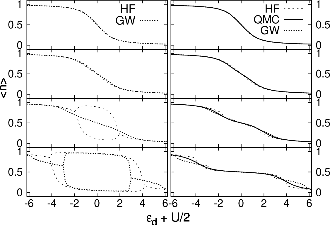
Fig. 1 shows the d-occupancy as a function of (the shift puts the particle-hole symmetric point at zero). The left panel shows the level occupancy obtained from the HF and GW approximations. The unphysical magnetic solutions occurring at are visible as a difference between and . (The QMC calculations yield at all () studied). For the parameters studied, . The depends more strongly on temperature than does making it difficult to determine with precision. We find at . The larger for the GW approximation arises from the self-consistency (using rather than to compute ); the renormalization of the Green function suppresses the instability White92; Suhl67.
The magnetic phase transition is an artifact of the HF and GW approximation schemes, but one may expect that the spin-averaged quantities are reasonably reliably represented. In the right column we plot the spin averaged . For strong interaction one can see clearly the Coulomb blockade plateau. All three methods yield a roughly correct shape for the occupancy vs level energy curve, in particular giving approximately correct widths for the Coulomb blockade plateau. At very weak interaction strength, () all three methods agree in detail. As the interaction is increased, differences appear between the approximate and exact results. The differences are most pronounced near the edges of the Coulomb blockade plateau, in the mixed valence regime where charge fluctuations are significant.
IV.2 Spectral function
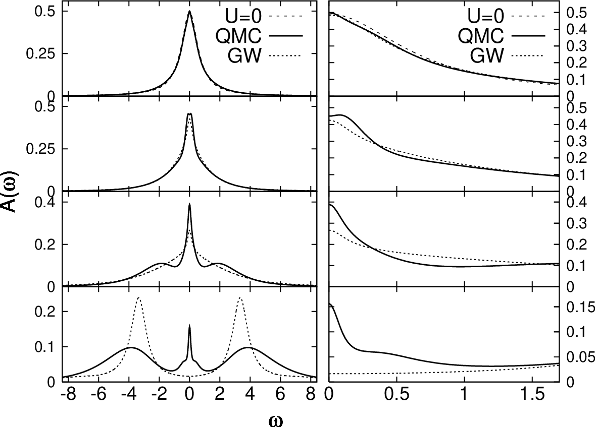
The computed spectral function is shown in Fig. 2. Focus first on the QMC results over the wide frequency range (left panels, solid lines). At the spectral function is very close to the non-interacting value. Moving to the middle panel, we see that when is increased from to , the Hubbard bands begin to form, however a central peak remains. At the height of the central peak should be . The reduced height is an effect of the non-zero temperature used in the simulations. For , Eq. (14) implies approximately equal to the studied . For the Hubbard band is well formed, and the central peak now clearly interpreted as a “Kondo resonance” remains. It is interesting that traces of the Kondo resonance are visible even though the temperature studied is much greater than the Kondo temperature estimated from Eq. (14) as previously noted by Meir et al Meir1993.
The dotted lines in Fig. 2 show the results of the GW approximation. The left panels show that GW agrees reasonably well with the exact results at , but at the GW does not produce the Hubbard bands and underestimates the hight of the central peak. At the GW approximation by contrast produces the Hubbard bands but misses the central peak. The right column is an expanded view of the central peak. For the two methods agree well with each other, essentially because the interaction corrections are weak. As the correlations are increased, differences appear. We see that even in the regime where the GW approximation is reasonably accurate, the low frequency lineshape is incorrect, with being too low near and too high in the wings of the central peak. The differences become more severe for higher .
IV.3 Conductance
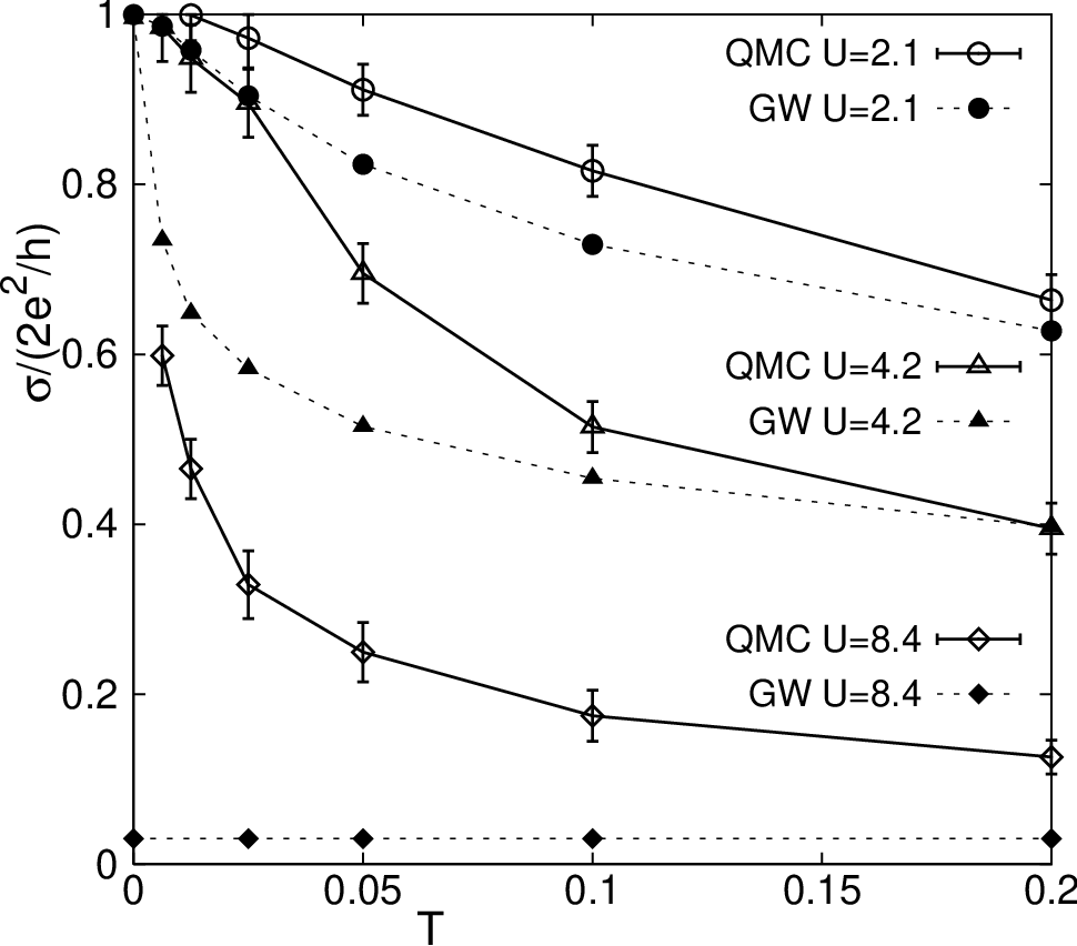
Figure 3 compares the QMC and GW predictions for the linear response conductance at several values. We see that the GW approximation systematically underestimates the conductance, with noticeable differences from the QMC values even for the smallest -value, , where the GW and QMC spectral functions agree reasonably well. We also note that general Fermi-liquid arguments imply that as , with a temperature scale of order . However, none of the calculations reveal a clear behavior except for the QMC calculations at ; we expect that this is because in all of the other cases the Kondo temperature is close to or below the temperatures studied.
The three panels of Fig. 4 show the dependence of on level position at two different temperatures. At we expect an approximately Lorentzian resonance lineshape, broadened from the non-interacting value by the density-dependent level-shift encoded in the real part of the self-energy. As is increased the conductance decreases; the decrease from the value is a consequence of many-body scattering; It is expected to be most pronounced at the particle-hole symmetric point . This may be seen mathematically from Eq. (14) for the Kondo temperature. In physical terms, the conductance involves valence fluctuation from the state to or ; at the half filled point, these states are most widely separated in energy, so the fluctuations are most easily disrupted by temperature.


The top panel shows results for , along with the curve for comparison. The increased width of the interacting curve relative to the noninteracting one is evident as is the approximately Lorenztian form. The GW and QMC results agree in the wings of the curve, but disagree in the small regime, with the GW approximation overestimating the suppression of conductance by thermal fluctuations.
The middle panel shows results for at two different temperatures. The QMC curves display the theoretically expected evolution with temperature and level position. In the wings of the lineshape (say for ) the curves are temperature independent (for the temperatures studied) and have an approximately Lorentzian decay. In the central region () the curves shown in Fig. 1 indicate the beginning of a Coulomb blockade plateau and we see correspondingly a strongly temperature dependent suppression of the conductance. For these parameters the Kondo temperature estimated from Eq. (14) is for ; we see that for our lower temperature the conductance approaches the noninteracting value, as expected. While the GW approximation shows dependence, it is too small for while extending strong dependence too far with respect to the level position. The shape of the -dependence of the conductance for a given is generally wrong through the Coulomb blockade region.
Finally, the lowest panel shows results for the strongest coupling, . Reference to Fig. 1 shows that for this interaction strength, the Coulomb blockade plateau is well formed. The theoretically estimated Kondo temperature at is rather lower than the lowest temperature studied; correspondingly the QMC conductance in the Coulomb blockade regime is small and strongly temperature dependent. In this regime the GW approximation predicts a magnetic state with a gap at the Fermi energy and no Kondo resonance, so that the conductance at small is qualitatively incorrect. The GW approximation produces the correct scale of at which conductance is restored (because it produces a Coulomb blockade plateau of the correct width) but gives an incorrect description of the details of the conductance as a function of level position until beyond the edge of the plateau.
IV.4 Self energy

Figure 5 shows the real frequency behavior of the self energy. We observe that the low frequency part of is linear with a negative slope, which is consistent with Eq. (15), and the statement that . QMC and GW give essentially the same values of for all interaction strengths shown. The weak structure visible for the smallest near is a numerical artifact of the analytical continuation. At higher frequencies differences between GW and QMC are evident. In particular, the high frequency tail of the GW curve disagrees with the exact analytical result (see Fig. 7 below). Turning now to the imaginary part of the self energy we first note that the low frequency part of is approximately quadratic, which is consistent with Eq.(15). Again the weak structures visible very close to are believed to be artifacts of the analytical continuation procedure. The non-zero value at is a temperature effect. The QMC is highly peaked; however GW fails to produce these peaks.
V Analysis of the GW approximation

In this section the input to the GW approximation is compared to the QMC results. The results provide an explicit measure of the relative importance of the neglected diagrams for the irreducible polarizability and the self energy.
Figure 6 compares the screened interaction obtained from the GW equation Eq. (21) to the obtained from the QMC calculation (Eq. (22)) for at the half filling point . We see that the interaction strongly increases as ; this is a signature of the slow spin fluctuations which are important to the physics. The charge fluctuations are suppressed by the Coulomb blockade effect. Remarkably, the exact and GW results agree very well at the lowest frequencies (see inset). However, the from the GW approximation is too large at intermediate to large frequencies; screening is incorrectly estimated. The ratio is also shown. The ratio quantifies the effect of vertex corrections, which are neglected in the GW approximation. The ratio becomes a constant above a certain frequency.


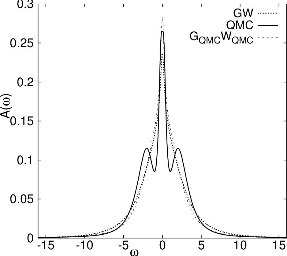
As shown in the Appendix, the GW approximation gives an incorrect treatment of the high frequency tail of the self energy, implying a violation of the Pauli principle. To fix this one may consider replacing the self-consistently determined and in Eq. (17) by the exact Green function and polarizibility. We have used our QMC simulations to measure and (from Eq. (22)) and used the results to compute from Eq. (17). Representative results are shown in Fig. 7. The upper panel shows the imaginary axis self energy. The GW curve is seen to have an incorrect asymptotic behavior. Using the QMC and produces a curve with the correct high frequency limit but with an incorrect low frequency behavior. A similar effect is seen in the lower panels, which display the analytically continued curves. Both GW and “” curves substantially underestimate the frequency dependence of . Additional insight comes from the spectral functions shown in Fig 8. We see that the “” curve fails to reproduce the Hubbard band structure, and gives an incorrect magnitude at low frequency.
This comparison explicitly shows that the diagrams neglected in the GW approximation for the self energy are significant in this regime. The use of the automatically includes the vertex corrections for the screened interaction. Approximations beyond GW also include vertex corrections explicitly in the expression for the self energy Hedin65; Hedin69. Figures 6-8 highlight the role they play for .
VI Conclusion
In this paper we used a numerically exact Quantum Monte Carlo method to obtain results for the density, conductance and spectral function of the single-impurity Anderson model, a simple theoretical paradigm problem for molecular conductors. The Anderson model is characterized by two dimensionless combinations of three parameters: a level position , a level width and an interaction . In the conventions adopted in this paper, the impurity level is half filled when . A relevant measure of the interaction strength is provided by the Hartree-Fock approximation, which predicts a magnetic state for interaction strengths greater than a critical value. We define to be the critical value for the half filled level. For the impurity spectral function is characterized by a three-peak structure with upper and lower Hubbard bands at and a central “Kondo” peak which controls the linear response conductance.
Our results are intended as benchmarks against which other, more approximate but more widely applicable methods may be compared. We compared our results to those obtained from the GW approximation, a self-consistent partial resummation of diagrammatic perturbation theory. The GW method is attractive because it can be combined with band theory to yield material-specific results, but its efficacy at treating strong correlations is unclear. Recent literature has argued that the GW method provides a reasonable description of the physics of the low ( limit) transport properties of molecular conductors for a range of intermediate Thygesen07a; Thygesen07b.
We showed that for weak to moderate coupling regime () or for a nearly full or nearly empty -level, the GW approximation provides a reasonable description. As the interaction approaches , some systematic deviations are observed in the shape of the spectral function near and the dependence of the conductance on the level position near . For the intermediate coupling regime () and the strong coupling regime (), the GW appproximation gives an inaccurate representation of the spectrum and the linear response conductance across the Coulomb blockade plateau. The accuracy is also limited for the mixed valence regions at the boundaries.
These findings are summarized in Fig. 9, which shows the regions where GW does and does not work well in the plane of interaction strength and level position. “Works well” is of course an imprecise definition; in constructing Fig. 9 we defined “works well” as “GW conductance within 15% of QMC conductance at ”. The criterion is temperature dependent as can be seen from Fig. 3 and interaction dependent, as can be seen from slope of the boundary line, which is less than . We find that the GW approximation is reliable when the level is tuned so that the density is far enough outside the Coulomb blockade region. For the GW approximation becomes reasonable for densities at the edge of the Coulomb blockade plateau, but for the density must be tuned well away from the plateau before GW becomes accurate.
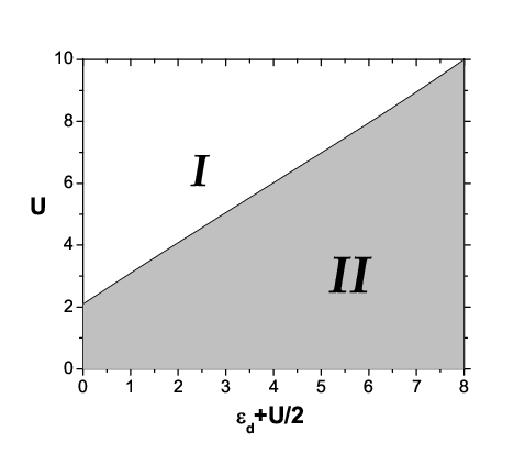
Qualitatively, in the parameter regime in which GW produces a central peak in the spectral function, it does not produce the Hubbard sidebands, while the Hubbard sidebands are produced only as a consequence of an unphysical magnetic ordering instability. Papers in the literature interpret the central peak found in the non-magnetic GW calculation as a Kondo resonance. We believe this interpretation is not correct. It is interesting to note, however, that some aspects of the many body physics (for example the low frequency “mass renormalization” or the spin correlation function) are correctly given by GW. This has been seen for the self consistent second order self energy as well White92.
The self consistent GW approximation has the virtue of being a conserving approximation Baym61; Baym62. In physical systems where the local molecular levels remain nearly filled or nearly empty, or where the hybridization is large, our results show that the GW approximation will be reasonably accurate. This suggests that an approach based on the GW approximation may be very useful for molecular conductors in the non-resonant tunneling regime where large discrepencies exist between theory and experiment. However, when the local Coulomb interactions on the molecule are strong, the GW approximation does not accurately represent the impact of local spin and charge fluctuations. Neither the spectral distribution nor the linear response conductance are given properly. Application of the GW approximation to nanoscale junctions in the Kondo regime is not well justified. The analysis of the screened Coulomb interaction and the evaluation of the GW approximation for the self energy operator with the the exact (QMC) and showed that vertex corrections are quite significant in these cases. Unfortunately, while there are systematic guidelines for including vertex corrections properly so as to maintain a conserving approximation, the resulting theory is substantially more complex Bickers89.
Our conclusions are based on linear response. Other situations, in particular the out-of-equilibrium Coulomb Blockade regime remain to be studied.
Acknowledgements We thank D. Reichman for helpful conversations. XW thanks A. Comanac and P. Werner for discussions and computer help. CDS thanks K. S. Thygesen for sharing details about the Pulay mixing implementation. This work was primarily supported by the Nanoscale Science and Engineering Initiative of the National Science Foundation under NSF Award Number CHE-0641523 and by the New York State Office of Science, Technology and Academic Research (NYSTAR). This work was partially supported by the US Department of Energy, Office of Basic Energy Sciences, under contract number DE-AC02-98CH10886 and by the National Science Foundation under grant number DMR-0705847.
Appendix
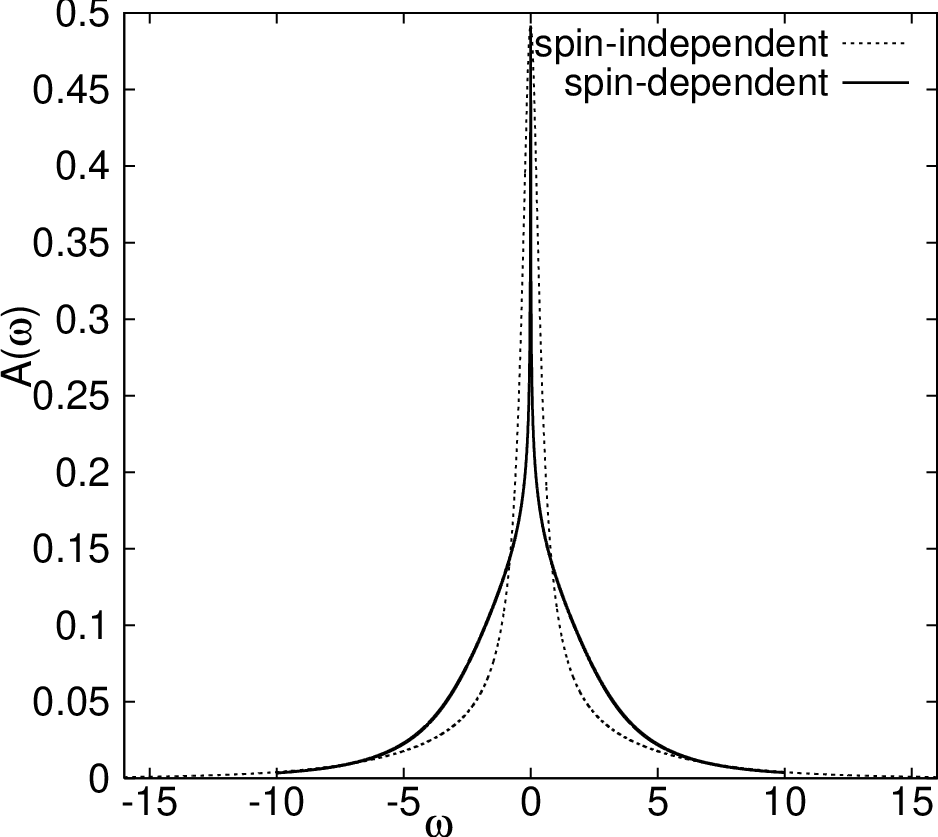
This Appendix discusses technical details of the GW calculations. The local interaction depends on electron spin. One may consider two forms:
| (A-1) | |||||
| (A-2) |
We now show that the asymptotic high-frequency behavior of the GW self energy implies that the spin-dependent interaction Eq. (A-2) is more appropriate than the spin-independent interaction Eq. (A-1).
It is convenient to separate out the Hartree and Fock terms, writing . For the spin-independent interaction the Hartree term for spin is while the Fock term is ; for the spin dependent interaction the Fock term vanishes and the Hartree term is . In either case we have
| (A-3) | |||||
where TO stands for time-ordered. In the exact perturbation theory analysis, the screened interaction is related to the spin-spin correlation function through the polarizability Fetter:
| (A-4) |
where:
| (A-5) |
In the spin-dependent case, the term in the interaction implies that involves only the correlator for the opposite spin, so one finds the following asymptotic behavior:
| (A-6) |
On the other hand, for the spin-independent interaction, all spin indices are involved and one obtains
Thus we see that the spin-dependent interaction reproduces approximately the analytically known asymptotic behavior of the self-energy whereas the spin-independent interaction does not. The asymptotic behavior is only approximately reproduced because GW cannot account correctly for . We show in the main text that using the exact yields the correct asymptotic behavior of but still does not produce an accurate approximation at general . The spin-independent case provides a much worse approximation, which would be wrong even if the exact correlations functions were used. This is an indication that the spin-dependent 2-particle interaction is to be prefered over the spin-independent one in the context of the GW approximation applied to the Anderson model.
Fig. 10 shows a comparison of spin-dependent and spin-independent GW at zero temperature. Comparison to the lowest temperature QMC result shows that the lineshape calculated from the spin-dependent GW approximation is closer to the QMC lineshape than is the result of the spin-independent calculation. This is because the spin-dependent approach is free of self-interaction effects and it accounts for some of spin-spin quantum fluctuations, whereas the spin-independent approach accounts only for density-density quantum fluctuations.
References
- (1) A. Nitzan and M. A. Ratner, Science 300, 1384 (2003).
- (2) L. Olesen, E. Laegsgaard, I. Stensgaard, F. Besenbacher, J. Schiotz, P. Stoltze, K. W. Jacobsen, and J. K. Norskov, Phys. Rev. Lett. 72, 2251 (1994).
- (3) A. Salomon, D. Cahen, S. Lindsay, J. Tomfohr, V. B. Engelkes, and C. D. Frisbie, Adv. Mater. 15, 1881 (2003).
- (4) N. J. Tao, Nature Nanotechnology 1, 173 (2006).
- (5) J. Park, A. N. Pasupathy, J. I. Goldsmith, C. Chang, Y. Yaish, J. R. Petta, M. Rinkowki, J. P. Sethna, H. D. Abruna, P. L. McEuen, and D. C. Ralph, Nature 417, 722 (2002).
- (6) W. Liang, M. P. Shores, M. Bockrath, J. R. Long, and H. Park, Nature 417, 725 (2002).
- (7) L. H. Yu, Z. K. Keane, J. W. Ciszek, L. Cheng, M. P. Stewart, J. M. Tour, and D. Natelson, Phys. Rev. Lett. 93, 266802 (2004).
- (8) D. Natelson, “Single-molecule transistors,” in Handbook of Organic Electronics and Photonics, H.S. Nalwa, ed., American Scientific Publishers (2006).
- (9) S. Datta, Electronic Transport in Mesoscopic Systems, Cambridge University Press, New York (1995).
- (10) A. Nitzan, Annu. Rev. Phys. Chem. 52, 681 (2001).
- (11) J. B. Neaton, M. S. Hybertsen and S. G. Louie, Phys. Rev. Lett. 97, 216405 (2006).
- (12) S. K. Nielsen, M. Brandbyge, K. Hansen, K. Stokbro, J. M. van Ruitenbeek, and F. Besenbacher, Phys. Rev. Lett. 89, 066804 (2002).
- (13) R. H. M. Smit, Y. Noat, C. Untiedt, N. D. Lang, M. C. van Hemert, and J. M. Ruitenbeek, Nature 419, 906 (2002).
- (14) K. S. Thygesen and K. W. Jacobsen, Phys. Rev. Lett. 94, 036807 (2005).
- (15) J. Heurich, J. C. Cuevas, W. Wenzel, and G. Schon, Phys. Rev. Lett. 88, 256803 (2002).
- (16) K. Stokbro, J. Talyor, M. Brandbyge, J. L. Mozos, and P. Ordejon, Comput. Mater. Sci. 27 151 (2003).
- (17) J. Tomfohr and O. F. Sankey, J. Chem. Phys. 120, 1542 (2004).
- (18) H. Basch, R. Cohen, and M. A. Ratner, Nano Lett. 5, 1668 (2005).
- (19) L. Venkataraman, J. E. Klare, I. W. Tam, C. Nuckolls, M. S. Hybertsen and M. Steigerwald, Nano Lett. 5, 458 (2006).
- (20) S.-Y. Quek, L. Venkataraman, H.J. Choi, S.G. Louie, M.S. Hybertsen and J.B. Neaton, Nano Lett. X, ASAP (2007).
- (21) C. Toher, A. Filippetti, S. Sanvito, and K. Burke, Phys. Rev. Lett. 95, 146402 (2005).
- (22) S.-H. Ke, H. U. Baranger and W. Yang, J. Chem. Phys. 126, 201102 (2007).
- (23) C. Toher and S. Sanvito, Phys. Rev. Lett. 99, 056801 (2007).
- (24) P. Delaney and J. C. Greer, Phys. Rev. Lett. 93, 036805 (2004).
- (25) B. Muralidharan, A. W. Ghosh, and S. Datta, Phys. Rev. B 73, 155410 (2006).
- (26) N. Sai, M. Zwolak, G. Vignale, and M. Di Ventra, Phys. Rev. Lett. 94, 186810 (2005).
- (27) M. Koentopp, K. Burke, and F. Evers, Phys. Rev. B 73, 121403(R) (2006).
- (28) A. Ferretti, A. Calzolari, R. Di Felice, F. Manghi, M. J. Caldas, M. Buongiorno Nardelli, and E. Molinari, Phys. Rev. Lett. 94, 116802 (2005).
- (29) A. Ferretti, A. Calzolari, R. Di Felice, and F. Manghi, Phys. Rev. B 72, 125114 (2005).
- (30) P. Darancet, A. Ferretti, D. Mayou, and V. Olevano, Phys. Rev. B 75, 075102 (2007).
- (31) K.S. Thygesen, A. Rubio, J. Chem. Phys. 126, 091101 (2007).
- (32) K. S. Thygesen and A. Rubio, arXiv:cond-mat/0710.0482
- (33) P. W. Anderson, Phys. Rev. 124, 41 (1961).
- (34) L. Hedin, Phys. Rev. 139, A796 (1965).
- (35) L. Hedin and S. Lundqvist, Solid State Phys. 23, 1 (1969).
- (36) M. S. Hybertsen and S. G. Louie, Phys. Rev. B 34, 5390 (1986).
- (37) F. Aryasetiawan, O. Gunnarsson, Rep. Prog. Phys. 61 237 (1998) and references therein.
- (38) W. G. Aulbur, L. Jonsson, and J. W. Wilkins, in Solid State Physics, edited by H. Ehrenreich and F. Spaepen (Academic, New York, 2000), p. 2, and references therein.
- (39) A. Stan, N. E. Dahlen and R. Van Leeuwen, Europhys. Lett. 76, 298 (2006).
- (40) M. van Schilfgaarde, T. Kotani and S. Faleev, Phys. Rev. Lett. 96, 226402 (2006).
- (41) G. Baym and L. P. Kadanoff, Phys. Rev. 124, 287 (1961).
- (42) G. Baym, Phys. Rev. 127, 1391 (1962).
- (43) G.D. Mahan, Many Particle Physics, 3rd Ed., Plenum (New York, 2000).
- (44) Y. Meir and N.S. Wingreen, Phys. Rev. Lett. 68, 2512 (1992).
- (45) P. Coleman, arXiv:cond-mat/0206003 v3 (2002)
- (46) J. Kondo, Prog. Theor. Phys. , 37 (1964)
- (47) K. G. Wilson, Rev. Mod. Phys. 47, 773 (1975)
- (48) F. D. M. Haldane, J. Phys. C: Solid State Physics 11, 5015 (1978)
- (49) L. X. Benedict, C. D. Spataru and S. G. Louie, Phys. Rev B , 085116 (2002).
- (50) A. L. Fetter and J. D. Walecka, Quantum Theory of Many-Particle Systems, (Dover, New York, 2003).
- (51) P. Pulay, Chem. Phys. Lett. , 393 (1980)
- (52) J. E. Hirsch and R. M. Fye, Phys. Rev. Lett. 56, 2521(1986)
- (53) A. Georges, G. Kotliar, W. Krauth and M. J. Rozenberg, Rev. Mod. Phys. 68, 13(1996)
- (54) P. Werner, A. Comanac, L. de’ Medici, M. Troyer and A. J. Millis, Phys. Rev. Lett. 97, 076405(2006)
- (55) P. Werner and A. J. Millis, Phys. Rev. B 74, 155107(2006)
- (56) M. Jarrell, J. E. Gubernatis, Phys. Rep. 269, 133 (1996)
- (57) J.A. White, Phys. Rev. B , 1100 (1992).
- (58) H. Suhl, Phys. Rev. Lett. 19, 442 (1967).
- (59) Y. Meir, N. S. Wingreen and P. A. Lee, Phys. Rev. Lett. , 2601 (1993).
- (60) N. E. Bickers and D. J. Scalapino, Annals of Physics (New York) , 206 (1989).