Fano resonance in a two-level quantum dot side-coupled to leads

Fano resonance, Fano61 which is the interference between a resonant state and a continuum, appears ubiquitously in various systems. It has a lineshape of the form

Here, $\varepsilon=(\omega-\xi_{0})/\Gamma$ is the detuning parameter measuring energy $\omega$ from the resonance center $\xi_{0}$ and normalized by the resonance half-width $\Gamma$, and $q$ is the Fano parameter characterizing lineshape asymmetry. For $q\rightarrow\infty$ Eq. (1) becomes the Breit-Wigner form, while for $q=0$ it shows an antiresonance. In general, $q$ is a complex quantity. Clerk01

Recently, Fano resonance has been investigated in mesoscopic electron systems such as waveguides, Tekman93 quantum dots, Gores00; Zacharia01 Aharonov-Bohm rings coupled to a quantum dot, Kobayashi02; Kobayashi04; Fuhrer06 and carbon nanotubes. Kim03; Yi03 The studies imply that Fano resonance provides a useful tool studying dephasing. Clerk01 On the other hand, some aspects of the interplay between Fano resonance and Coulomb interaction have been studied. They include Fano resonance modified by charge sensing Johnson04; Stefanski05 and Fano-Kondo antiresonance in a spin-degenerate single-level quantum dot. Bulka01; Hofstetter01; Sato05

The Fano lineshape (1) is applicable for a system with a single resonant level. It is valid as well for multilevel systems as long as each single-particle level is well separated from the adjacent levels in energy. Most studies on Fano resonance have been carried out mainly in this single-level regime. However, one may often find the multilevel regime where single-particle level spacing is comparable to level broadening. In this regime, the single-level Fano form is not applicable any more. Moreover, this regime possesses interesting effects, absent in the single-level regime, such as nonmonotonic level occupation Berkovits05; Konig05; Sindel05 due to Coulomb repulsion. It has been reported Goldstein06 that the nonmonotonic behavior of level occupation influences Breit-Wigner lineshape. Therefore, it may be interesting to see the modification of resonance lineshape, from Eq. (1), in a more general multilevel Fano regime and to analyze the influence of Coulomb interaction on resonance lineshape, which is the aim of the present paper.

In this work, we theoretically study Fano resonance in a two-level electron quantum dot (QD) side-coupled to two leads, which are connected by a direct channel (see Fig. 1). Interlevel Coulomb repulsion in the dot is taken into account and the spin of electrons is neglected for simplicity. We use Keldysh formalism and a self-consistent Hartree-Fock (SCHF) approach, to obtain and to analyze the Fano resonance lineshape of the two-level system. The two-level lineshape is found to be deformed from the single-level form (1) by the Coulomb repulsion and interlevel interference. We derive the connection [Eqs. (14) to (16)] between the lineshape deformation and the nonmonotonicity of level occupation, when the QD level spacing (after renormalized by the repulsion) is larger than level broadening so that the nonmonotonicity is not too strong. The connection may be useful for experimental study. We also discuss the dependence of the nonmonotonicity on the direct-channel coupling, an extension to a spinful single-level case, and the temperature range where the SCHF result is valid, below which correlation-induced resonances Meden06; Karrasch06; Lee07; Kashcheyevs07; Silvestrov07 may emerge.

We start with the Hamiltonian $H_{D}$ of the spinless two-level QD,

where $d^{\dagger}_{\gamma}$ creates an electron at QD level $\gamma=1,2$ with energy $\xi_{\gamma}$, $V_{g}$ is the gate voltage applied to the QD, and $U$ is the interlevel Coulomb repulsion. Without loss of generality, we can set $\xi_{1}<\xi_{2}$. The QD couples via tunneling to noninteracting leads $\alpha=L,R$, which are connected by a direct channel (see Fig. 1), so that the total Hamiltonian of the system is $H=H_{D}+H_{L}+H_{TD}+H_{TL}$, where the two leads, the dot-lead tunneling, and the lead-lead tunneling are described by $H_{L}=\sum_{k,\alpha}\xi_{k\alpha}c_{k\alpha}^{{\dagger}}c_{k\alpha}$, $H_{TD}=\sum_{k\alpha\gamma}(t_{\alpha\gamma}c_{k\alpha}^{{\dagger}}d_{\gamma}+\mathrm{h.c.})$, and $H_{TL}=\sum_{kk^{\prime}}(t_{LR}c_{kL}^{{\dagger}}c_{k^{\prime}R}+\mathrm{h.c.})$, respectively. Here $c_{k\alpha}^{\dagger}$ creates an electron with momentum $k$ and energy $\xi_{k\alpha}$ at lead $\alpha$. We ignore for simplicity the momentum dependence of tunneling matrix elements $t_{\alpha\gamma}$ between level $\gamma$ and lead $\alpha$, and that of $t_{LR}$ of the direct channel.

It is worthwhile to note that electron transport through the two levels depends on the dot-lead coupling $t_{\alpha\gamma}$. To see this, we consider simple cases Silva02 with time reversal symmetry where $t_{\alpha\gamma}$’s are chosen to be real, $t_{L1}=t_{R1}=t_{1}>0$, $t_{L2}=st_{R2}=t_{2}>0$, and the phase parameter $s=\pm 1$. After redefining a pair of two orthogonal leads, saying $\tilde{\alpha}=\pm 1$, by $\tilde{c}_{k\tilde{\alpha}}=(c_{kL}+\tilde{\alpha}c_{kR})/\sqrt{2}$, one finds that for $s=+1$, the two QD levels couple to the same lead $\tilde{\alpha}=+1$, while for $s=-1$, they couple to different leads each other. This $s$-dependent nature of coupling to leads $\tilde{\alpha}$ characterizes Silva02; Sindel05; Goldstein06 electron transport such as interference. Below, we will use the above choice of $t_{\alpha\gamma}$’s and see the dependence of the two-level Fano lineshape on $s$. Note that $t_{LR}$ is also chosen to be real as well.

We obtain electric current of the QD system using Keldysh formalism. Meir92 The current, $J_{L}=-e\langle\dot{n}_{L}\rangle=(ie/\hbar)\langle[n_{L},H]\rangle$, in the lead $L$ can be expressed as

Here, $n_{L}\equiv\sum_{k}c_{kL}^{{\dagger}}c_{kL}$ is the electron density operator, and $G^{<}(\omega)$’s are lesser Green’s functions which correspond in time domain to $G_{\gamma,kL}^{<}(t,t^{\prime})\equiv i\langle c_{kL}^{\dagger}(t^{\prime})d_{\gamma}(t)\rangle$ and $G_{k^{\prime}R,kL}^{<}(t,t^{\prime})=i\langle c_{kL}^{\dagger}(t^{\prime})c_{k^{\prime}R}(t)\rangle$. One finds the current $J_{R}$ in lead $R$ in the same way. After some algebra Meir92 using the relations connecting $G^{<}$’s and the retarded Green function $G^{r}_{\gamma\gamma^{\prime}}$ of the QD [see Eqs. (8) and (9)], the wide-band approximation for lead Green’s function $g_{k\alpha}$, $\sum_{k}g_{k\alpha}^{r}(\omega)\simeq-i\pi\rho$, $\rho$ being the density of states of leads, and the steady-state current conservation $J_{L}=-J_{R}$, we arrive at a useful form of the current,

where $f_{\alpha}$ is the Fermi distribution of lead $\alpha$. The background transmission, $\mathcal{T}_{B}=4\pi^{2}\rho^{2}t_{LR}^{2}/x^{2}$, comes only from the direct channel, where $x=1+\pi^{2}\rho^{2}t_{LR}^{2}$ is the factor counting multiple reflections via the direct channel. The term $\mathcal{T}_{QD}$ results from the paths passing through the QD, and it depends on the phase parameter $s$,

where $y=(1-i\pi\rho t_{LR})^{4}/x^{2}$ is a complex factor coming from the effect of the direct channel and

is the QD level broadening. Bulka01; Hofstetter01 Notice that $\tilde{\Gamma}_{\gamma}$ becomes narrower, as $t_{LR}$ increases, from the level broadening $\Gamma_{\gamma}=2\pi\rho t^{2}_{\gamma}$ of the QD without the direct channel. The first two terms of Eqs. (5,6) describe the direct contribution through the QD level $\gamma$ as well as the interference between the paths through the level $\gamma$ and the direct channel, while the third shows the interlevel interference between the paths through the two levels.

The derivation of $\mathcal{T}_{QD}$ depends on $s$ due to the coupling nature to the leads $\tilde{\alpha}$. For $s=-1$, $G_{12}^{r}$ does not appear in $\mathcal{T}_{QD}$, and it is necessary to use Keldysh equation $G^{<}=G^{r}\Sigma^{<}G^{a}$ for the dot lesser function. We use the noninteracting form of the lesser self-energy $\Sigma^{<}$ of the dot coming from the lead-dot coupling, therefore $\mathcal{T}_{QD}^{s=-1}$ in Eq. (6) is an approximate form valid within the SCHF approach used below. On the other hand, for $s=+1$, the Keldysh equation is not necessary in the derivation, thus $\mathcal{T}_{QD}^{s=+1}$ in Eq. (5) is exact. Note that Eqs. (4,5,6) are reduced into the forms found in the previous works on the single-level Fano resonance Bulka01; Hofstetter01 (when $\xi_{2}-\xi_{1}\gg\tilde{\Gamma}_{\gamma=1,2}$) and on a multilevel QD without the direct channel Meir92 ($t_{LR}\to 0$).

We obtain the retarded QD Green’s function $G^{r}_{\gamma\gamma^{\prime}}$ and the level occupation $\langle n_{\gamma\gamma^{\prime}}\rangle$ in equilibrium by using the equation of motion method and the SCHF approach,

where $\mathbf{D}=\big(\omega-\xi_{1}+eV_{g}-U\langle n_{2}\rangle-\Sigma_{1}^{r}\big)\big(\omega-\xi_{2}+eV_{g}-U\langle n_{1}\rangle-\Sigma_{2}^{r}\big)-\big(U\langle n_{12}\rangle-\Sigma_{12}^{r}\big)^{2}$, $\bar{\gamma}$ means the level different from $\gamma$, $\langle n_{\gamma}\rangle\equiv\langle n_{\gamma\gamma}\rangle$ is the occupation of level $\gamma$, and $f(\omega)=1/(e^{\beta\omega}+1)$. The self-energies are found to be $\Sigma_{\gamma}^{r}=-(s^{\gamma-1}\pi\rho t_{LR}+i)\tilde{\Gamma}_{\gamma}$ and $\Sigma_{12}^{r}=-\delta_{s,1}(\pi\rho t_{LR}+i)\sqrt{\tilde{\Gamma}_{1}\tilde{\Gamma}_{2}}$; from $\mathfrak{Im}\Sigma_{\gamma}^{r}$, one can get Eq. (7). We remark that $\Sigma_{12}^{r}$ and $\langle n_{12}\rangle$, therefore $G_{12}^{r}$, vanish for $s=-1$, because of the $s$-dependent coupling nature to the leads $\tilde{\alpha}$. The SCHF approach is good when $\Gamma_{\gamma}$ is not too large compared with level spacing $\xi_{2}-\xi_{1}$. Sindel05 We later discuss the temperature range where the SCHF result may be valid. Since we have interest in resonance lineshape, we will focus on the the linear response regime below.

We first discuss two-level resonance lineshape in the noninteracting case of $U=0$. The two-level lineshape can be obtained as $\mathcal{T}\equiv\mathcal{T}_{B}+\mathcal{T}_{QD}(\omega=0)$,

where $\varepsilon_{\gamma}=(eV_{g}-\xi_{\gamma})/\tilde{\Gamma}_{\gamma}+s^{\gamma-1}\pi\rho t_{LR}$ is the detuning parameter of level $\gamma=1,2$, $\zeta\equiv-(\tilde{\Gamma}_{1}\tilde{\Gamma}_{2})^{-1/2}\mathfrak{Re}\Sigma^{r}_{12}=\pi\rho t_{LR}\delta_{s,1}$, the terms with Kronecker delta $\delta_{s,1}$ come from $\Sigma_{12}^{r}$, $q\equiv\sqrt{(1-\mathcal{T}_{B})/\mathcal{T}_{B}}$, $s^{\gamma-1}q$ is the Fano parameter of the level $\gamma$. Note that the lineshape $\mathcal{T}$ is reduced into the single-level form (1) when the level spacing $\xi_{2}-\xi_{1}\ll\tilde{\Gamma}_{\gamma}$.

Figure 2 shows typical two-level Fano lineshapes as a function of gate voltage $V_{g}$ for the cases where $U=0$ and the level broadening $\tilde{\Gamma}_{\gamma}$ is comparable to the level spacing $\xi_{2}-\xi_{1}$. The entire lineshape may be understood as $s$-dependent mixture of interferences between the paths through one QD level and the direct channel (characterized by the Fano parameter of the level) and between the paths through the two QD levels. For $s=-1$, the upper resonance at $\xi_{2}$ has a negative value of Fano parameter, while the lower one at $\xi_{1}$ has a positive value. Therefore, the two resonances are out of phase (with difference by $\pi$), as shown in Fig. 2(a). On the other hand, for $s=+1$, the two resonances are in phase [see Fig. 2(b)].

In Fig. 2, we plot the cross-correlation of level occupation, Konig05 $\langle\delta n_{1}\delta n_{2}\rangle\equiv\langle n_{1}n_{2}\rangle-\langle n_{1}\rangle\langle n_{2}\rangle\simeq-\langle n_{12}\rangle^{2}$, which may give more understanding of the $s$-dependent features. For $s=+1$, $\langle\delta n_{1}\delta n_{2}\rangle$ can have a finite value and give rise to nonmonotonic behavior of $\langle n_{\gamma}\rangle$ [see $\langle n_{1}\rangle$ around $eV_{g}=\xi_{2}$ in Fig. 2(b)], while it vanishes for $s=-1$. Note that it becomes suppressed as $t_{LR}$ increases since the overlap between the two levels or the level broadening $\tilde{\Gamma}_{\gamma}$ is reduced [see Eq. (7)].

Hereafter we turn on the Coulomb repulsion $U$ and discuss how it modifies the resonance lineshape. We find that within the SCHF treatment, the lineshape has the same form as the noninteracting case of $U=0$, Eq. (11),

but with mean-field shifts

Note that $\varepsilon_{\gamma}$ and $\langle n_{\gamma\gamma^{\prime}}\rangle$ depend on $V_{g}$. The shift of the detuning parameter can be understood as the level spacing renormalization due to the Hartree repulsion. On the other hand, the shift in $\tilde{\zeta}$ comes from the Fock exchange, which is absent in the case of $s=-1$.

In Figs. 3(a) and (b), we plot the lineshape $\mathcal{T}$ when nonmonotonic behavior Berkovits05; Konig05; Sindel05; Goldstein06 of $\langle n_{\gamma}\rangle$ occurs (see, e.g., $\langle n_{1}\rangle$ around the second resonance). For $s=+1$, the nonmonotonic behavior comes from the Hartree repulsion as well as from the Fock exchange, while for $s=-1$, it is caused only by the former. Therefore, the $s=+1$ case shows the nonmonotonicity in a wider range of $V_{g}$ where $\langle\delta n_{1}\delta n_{2}\rangle$ is enhanced by the Fock exchange.

The nonmonotonic dependence of $\langle n_{\gamma\gamma^{\prime}}\rangle$ on $V_{g}$ modifies the lineshape from the noninteracting cases. Such modification can be analyzed when the level spacing renormalized by the Hartree contribution is much larger than level broadening $\tilde{\Gamma}_{\gamma}$, i.e., when $\xi_{2}-\xi_{1}+U\gg\tilde{\Gamma}_{\gamma}$, so that the nonmonotonicity is not too strong. In this case, the lineshape (12) can be simplified, for gate voltage, for example, around the second resonance ($eV_{g}\simeq\xi_{2}+U+s\pi\rho t_{LR}\tilde{\Gamma}_{2}$), into the single-level Fano form $\mathcal{T}_{0}$,

but with not simple dependence of $\langle n_{1}\rangle$ on $V_{g}$ [see Eq. (13)]. To analyze further, we define nonmonotonicity measure

Here, $\langle n_{1}\rangle_{0}(V_{g})$ is the level occupation in the absence of the Coulomb repulsion, which can be obtained from Eqs. (8,9,10). We can take $\langle n_{1}\rangle_{0}(V_{g})\simeq 1$ in this case of large renormalized level spacing. For $|\Delta|\ll 1$, one has an approximated form of the lineshape,

The leading term $\mathcal{T}_{0}$ obeys the single-level Fano form (1) with the detuning parameter $\tilde{\varepsilon}_{2,0}=(eV_{g}-\xi_{2}-U\langle n_{1}\rangle_{0})/\tilde{\Gamma}_{2}+s\pi\rho t_{LR}\simeq(eV_{g}-\xi_{2}-U)/\tilde{\Gamma}_{2}+s\pi\rho t_{LR}$, which approximately linearly depends on $V_{g}$, and the second deformation term is proportional to $\Delta(V_{g})$, therefore it provides the connection between the lineshape and the nonmonotonicity. Around the first resonance, one can find the same forms of the connection and the nonmonotonicity measure but with level index exchange $1\leftrightarrow 2$ and $\langle n_{2}\rangle_{0}\simeq 0$. The connection is applicable as well in the Breit-Wigner case of $\mathcal{T}_{BW,0}=\mathcal{T}_{0}(t_{LR}\to 0)$.

In Figs. 3(c) and (d), we plot the deviation of $\mathcal{T}$ from $\mathcal{T}_{0}$ as well as $\Delta$. The deviation depends on the phase parameter $s$, as the nonmonotonicity does. The lineshape deformation occurs in a wider range of $V_{g}$ in the case of $s=+1$, since the Fock exchange enhances $\langle\delta n_{1}\delta n_{2}\rangle$ and therefore additional nonmonotonicity only in the $s=+1$ case, as discussed before. The connection between the lineshape deformation and the nonmonotonicity of level occupation found in Eq. (16) may suggest an experimental study of the nonmonotonic behavior.

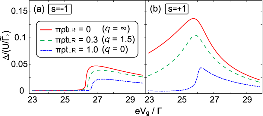
We finally discuss a few remarks briefly. First, the nonmonotonic behavior becomes weakened for larger direct channel coupling $t_{LR}$, because the level broadening $\tilde{\Gamma}_{\gamma}$ becomes narrower [see Fig. 4 and Eq. (7)]. Second, we extend the above findings to a spinful single-level QD. In this case, the Hartree repulsion induces the nonmonotonic behavior of level occupation, but there is no interlevel interference and no Fock contribution. We find that the connection (16) between the lineshape deformation and the nonmonotonicity is still hold (at temperatures larger than the Kondo temperature).

Third, the temperature range where the SCHF approach is valid depends on $t_{LR}$. It has been found Lee07; Kashcheyevs07; Silvestrov07 that when $t_{LR}=0$, the two-level QD can be mapped into a Kondo system and it can show correlation-induced resonance Meden06 below the Kondo temperature. We find that the two-level QD with the direct channel can be also mapped Lee into a Kondo system, depending on $s$, and that the corresponding Kondo temperature decreases with increasing $t_{LR}$. Therefore, our approach may be valid above the Kondo temperature, the upper bound of which can be estimated Lee07 from the case of $t_{LR}=0$.

In summary, we have studied Fano resonance lineshape and the nonmonotonicity of level occupation in a two-level QD side-coupled two leads. The two-level lineshape is derived for both the noninteracting and interacting cases [Eqs. (11,12)]. We especially obtain the connection, Eq. (16), between the nonmonotonicity and the Coulomb modification of the lineshape. We also find that stronger direct-channel coupling weakens the nonmonotonicity.

This work was supported by a Korean Research Foundation Grant (KRF-2006-331-C00118).

References

- (1) U. Fano, Phys. Rev. 124, 1866 (1961).
- (2) A. A. Clerk, X. Waintal, and P. W. Brouwer, Phys. Rev. Lett. 86, 4636 (2001).
- (3) E. Tekman and P. F. Bagwell, Phys. Rev. B 48, 2553 (1993); J. U. Nöckel and A. D. Stone, Phys. Rev. B 50, 17415 (1994).
- (4) J. Göres et al., Phys. Rev. B 62, 2188 (2000).
- (5) I. G. Zacharia et al., Phys. Rev. B 64, 155311 (2001).
- (6) K. Kobayashi et al., Phys. Rev. Lett. 88, 256806 (2002).
- (7) K. Kobayashi et al., Phys. Rev. B 70, 035319 (2004).
- (8) A. Fuhrer et al., Phys. Rev. B 73, 205326 (2006).
- (9) J. Kim et al., Phys. Rev. Lett. 90, 166403 (2003).
- (10) W. Yi et al., Phys. Rev. Lett. 91, 076801 (2003).
- (11) A. C. Johnson et al., Phys. Rev. Lett. 93, 106803 (2004).
- (12) P. Stefański, A. Tagliacozzo, and B. R. Bułka, Solid State Commun. 135, 314 (2005).
- (13) B. R. Bułka and P. Stefański, Phys. Rev. Lett. 86, 5128 (2001).
- (14) W. Hofstetter, J. König, and H. Schoeller, Phys. Rev. Lett. 87, 156803 (2001).
- (15) M. Sato et al., Phys. Rev. Lett. 95, 066801 (2005).
- (16) R. Berkovits, F. von Oppen, and Y. Gefen, Phys. Rev. Lett. 94, 076802 (2005).
- (17) J. König and Y. Gefen, Phys. Rev. B 71, 201308 (2005).
- (18) M. Sindel et al., Phys. Rev. B 72, 125316 (2005).
- (19) M. Goldstein and R. Berkovits, New J. Phys. 9, 118 (2007).
- (20) V. Meden and F. Marquardt, Phys. Rev. Lett. 96, 146801 (2006).
- (21) C. Karrasch, T. Enss, and V. Meden, Phys. Rev. B 73, 235337 (2006).
- (22) H.-W. Lee and S. Kim, Phys. Rev. Lett. 98, 186805 (2007).
- (23) V. Kashcheyevs et al., Phys. Rev. B 75, 115313 (2007).
- (24) P. G. Silvestrov and Y. Imry, Phys. Rev. B 75, 115335 (2007).
- (25) A. Silva, Y. Oreg, and Y. Gefen, Phys. Rev. B 66, 195316 (2002).
- (26) Y. Meir and N. S. Wingreen, Phys. Rev. Lett. 68, 2512 (1992).
- (27) W.-R. Lee, J. U. Kim, and H.-S. Sim, to be published.