As the nucleon is not a point-like spin-$\frac{1}{2}$ target with an anomalous magnetic moment, the photon field displaces in low-energy Compton scattering $\gamma N\to\gamma N$ its charged constituents, inducing a non-vanishing multipole-moment. These long-known nucleon-structure effects are for static external fields parameterised by the electric polarisability $\overline{\alpha}$ and its magnetic counter-part $\overline{\beta}$. For the proton, the generally accepted static values are $\overline{\alpha}^{p}\approx 12\times 10^{-4}\;\mathrm{fm}^{3},\;\overline{\beta}^{p}\approx 2\times 10^{-4}\;\mathrm{fm}^{3}$, with error-bars of about $1$. ¹¹ 1 It is customary to measure the scalar dipole-polarisabilities in $10^{-4}\;\mathrm{fm}^{3}$, so that the units are dropped in the following. Notice that the nucleon is quite stiff.

Does the neutron react similarly under deformations, $\overline{\alpha}^{p}\approx\overline{\alpha}^{n}$, $\overline{\beta}^{p}\approx\overline{\beta}^{n}$? Different types of experiments report a range of values $\overline{\alpha}^{n}\in[-4;19]$: Coulomb scattering of neutrons off lead, and deuteron Compton-scattering $\gamma d\to\gamma d$ with and without breakup, see e.g. [1] for a list. The latter should be a clean way to extract the iso-scalar polarisabilities $\overline{\alpha}^{s}:=\frac{1}{2}(\overline{\alpha}^{p}+\overline{\alpha}^{n})$ and $\overline{\beta}^{s}$ in analogy to determinations of the proton polarisabilities. Experiments were performed in Urbana at $\omega=49$ and $69$ MeV, in Saskatoon (SAL) at $94$ MeV, and in Lund (MAXlab) at $55$ and $66$ MeV. While all low-energy extractions are consistent with small iso-vectorial polarisabilities, the SAL data lead to conflicting analyses: The original publication [2] gave $\overline{\alpha}^{s}=8.8\pm 1.0$, using the Baldin sum-rule for the static nucleon polarisabilities. Without it, Levchuk and L’vov obtained $\overline{\alpha}^{s}=11\pm 2,\;\overline{\beta}^{s}=7\pm 2$ [3]; and Beane et al. found recently from all data $\overline{\alpha}^{s}=13\pm 4,\;\overline{\beta}^{s}=-2\pm 3$ [4]. The extraction being very sensitive to the polarisabilities, this seems discouraging news.

These notes outline the resolution of the puzzle and report on a new high-accuracy determination of the nucleon polarisabilities from all Compton scattering data. There are two main ingredients: a better understanding of dispersive effects in the polarisabilities themselves as discussed in Sect. 2; and a model-independent determination of meson-exchange current effects with an error-estimate, Sect. 3. As customary in proceedings, I apologise for my biased view and refer to [1] at least for a better list of references.

The nucleon-structure effects encoded by the polarisabilities are conveniently parameterised starting from the most general interaction between a nucleon $N$ with spin $\vec{\sigma}/2$ and an electro-magnetic field of fixed, non-zero energy $\omega$:

	$\displaystyle\mathcal{L}_{\text{pol}}=2\pi N^{\dagger}\big[{\alpha_{E1}(\omega)}\vec{E}^{2}+{\beta_{M1}(\omega)}\vec{B}^{2}+{\gamma_{E1E1}(\omega)}\vec{\sigma}\cdot(\vec{E}\times\dot{\vec{E}})$				(1)
			$\displaystyle\!\!\!\!\!\!\!+{\gamma_{M1M1}(\omega)}\vec{\sigma}\cdot(\vec{B}\times\dot{\vec{B}})-2{\gamma_{M1E2}(\omega)}\sigma_{i}B_{j}E_{ij}+2{\gamma_{E1M2}(\omega)}\sigma_{i}E_{j}B_{ij}+\dots\big]N$

Here, the electric or magnetic (${X,Y=E,M}$) photon undergoes a transition ${Xl\to Yl^{\prime}}$ of definite multipolarity ${l,l^{\prime}=l\pm\{0,1\}}$; ${T_{ij}:=\frac{1}{2}(\partial_{i}T_{j}+\partial_{j}T_{i})}$. Its coefficients are the energy-dependent or dynamical polarisabilities of the nucleon [5]. Most prominently, there are six dipole-polarisabilities. The two spin-independent ones parameterise electric and magnetic dipole-transitions, $\alpha_{E1}(\omega)$ and $\beta_{M1}(\omega)$. Particularly interesting are the four spin-polarisabilities $\gamma_{E1E1}(\omega)$, $\gamma_{M1M1}(\omega)$, $\gamma_{E1M2}(\omega)$, $\gamma_{M1E2}(\omega)$ as they parameterise the response of the nucleon-spin to the photon field. Contributions from higher ones like quadrupole polarisabilities are negligible in today’s experiments.

Polarisabilities measure the global stiffness of the nucleon’s internal degrees of freedom against displacement in an electric or magnetic field of definite multipolarity and non-vanishing frequency $\omega$ and are identified at fixed energy only by their different angular dependence. Nucleon Compton scattering provides thus a wealth of information about the internal structure of the nucleon. In contradistinction to most other electro-magnetic processes, the nucleon-structure effects in Compton scattering were however previously not analysed in terms of a multipole-expansion at fixed energies. Instead, one focused on the static electric and magnetic polarisabilities $\overline{\alpha}:=\alpha_{E1}(\omega=0)$ and $\overline{\beta}:=\beta_{M1}(\omega=0)$, which are often called “the polarisabilities”. While quite different frameworks could provide a consistent picture for them, the underlying mechanisms are only properly revealed by the energy-dependence.

Clearly, the complete set of dynamical polarisabilities does – like in all multipole-decompositions – not contain more or less information about the temporal response of the nucleonic degrees of freedom than the Compton amplitudes. But the information is better accessible and easier to interpret, as each mechanism leaves a characteristic signature in a particular channel.

To investigate them in a model-independent framework, we employ the unique low-energy theory of QCD, namely Chiral Effective Field Theory $\chi$EFT. It contains only those low-energy degrees of freedom which are observed at the typical energy of the process, interacting in all ways allowed by the underlying symmetries of QCD. A momentum expansion of all forces allows for model-independent results of finite, systematically improvable accuracy and thus for an estimate of the theoretical uncertainties encountered by neglecting higher-order contributions. The resulting contributions at leading order (LO) are listed in Fig. 1 and easily motivated [5]:

(1) Photons couple to the pions around the nucleon and around the $\Delta$, signalled by a characteristic cusp at the one-pion production threshold.

(2) It is well-known that the $\Delta(1232)$ as the lowest nuclear resonance leads by the strong $\gamma N\Delta$ $M1$-transition to a para-magnetic contribution to the static magnetic dipole-polarisability $\overline{\beta}_{\Delta}=+[7\dots 13]$ and a characteristic resonance-shape, cf. the Lorentz-Drude model of classical electrodynamics.

(3) As the observed static value $\overline{\beta}^{p}\approx 2$ is smaller by a factor of $5$ than the $\Delta$ contribution, a strong dia-magnetic component must exist. The resultant fine-tuning at zero photon-energy is unlikely to hold once the evolution with the photon energy is considered: If dia- and para-magnetism are of different origin, they involve different scales and hence different energy-dependences. We sub-sume this short-distance Physics which is at this order not generated by the pion or $\Delta$ into two energy-independent low-energy coefficients $\delta\alpha,\;\delta\beta$.

The cornucopia of Compton data on the proton below $200\;\mathrm{MeV}$ determines these to be indeed anomalously large, $\delta\alpha=-5.9\pm 1.4,\;\delta\beta=-10.7\pm 1.2$, justifying their inclusion at leading order. As expected, $\delta\beta$ is dia-magnetic. The resulting static proton polarisabilities

$$\displaystyle\overline{\alpha}^{p}=11.0\pm 1.4_{\mathrm{stat}}\pm 0.4_{\text{Baldin}}\;\;\;\;,\;\;\;\;\overline{\beta}^{p}=2.8\mp 1.4_{\mathrm{stat}}\pm 0.4_{\text{Baldin}}$$

(2)

compare both in magnitude and uncertainty favourably with other state-of-the-art results [5]. Higher-order corrections contribute an error of about $\pm 1$ not displayed here as the statistics dominates the total error.

That the two short-distance parameters $\delta\alpha,\;\delta\beta$ suffice to describe the data up to $\omega\approx 200\;\mathrm{MeV}$ [5] leads to three constraints on their explanation:

(1) Like $\delta\alpha,\;\delta\beta$, the effect must be $\omega$-independent over a wide range.

(2) Albeit it must lead to the values for $\delta\alpha,\;\delta\beta$ predicted in $\chi$EFT, it must be absent at least in the pure spin-polarisabilities $\gamma_{E1E1},\;\gamma_{M1M1}$.

(3) Its prediction for the proton and neutron must be similar because iso-vectorial effects are small and energy-independent [6, 5].

Power counting

Since free neutrons can often not be used in experiments, their properties are usually extracted from data taken on few-nucleon systems by dis-entangling nuclear-binding effects. $\chi$EFT allows to subtract two-body contributions from meson-exchange currents and wave-function dependence from data with minimal theoretical prejudice and an estimate of the theoretical uncertainties.

A consistent description must also give the correct Thomson limit, i.e. the exact low-energy theorem which is a consequence of gauge invariance [7, 8].

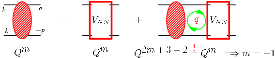
Its verification is straight-forward in the 1-nucleon sector, where the amplitude is perturbative. In contradistinction, the two-nucleon amplitude must be non-perturbative to accommodate the shallow bound-state: All terms in the LO Lippmann-Schwinger equation of $NN$-scattering, Fig. 3, including the potential, must be of the same order when all nucleons are close to their non-relativistic mass-shell. Otherwise, one of them could be treated as perturbation of the others and a low-lying bound-state would be absent. Picking the nucleon-pole in the energy-integration $E\sim\frac{\vec{k}^{2}}{2M}$ leads therefore to the consistency condition that the $NN$-scattering amplitude $T_{NN}$ must be of order $Q^{-1}$, irrespective of the potential used. $Q$ is a typical low-momentum scale of the process under consideration, e.g. the inverse $\mathrm{S}$-wave scattering length. It does therefore not suffice to determine the relative strength of forces and potentials in $\chi$EFT just by counting the number of momenta. This has long been recognised in “pion-less” EFT, but is only an emerging communal wisdom in the chiral version [9, 10, 11].

In deuteron Compton scattering, this mandates inclusion of $T_{NN}$ for all graphs in which both nucleons propagate close to their mass-shell between photon absorption and emission, i.e. in which the photon energy $\omega\lesssim 50\;\mathrm{MeV}$ does not suffice to knock a nucleon far off its mass-shell [1, 9]. Figure 4 lists the contributions to Compton scattering off the deuteron to next-to-leading order NLO in $\chi$EFT. At higher photon energies $\omega\gtrsim 60\;\mathrm{MeV}$, on can show that the nucleon is kicked far off its mass-shell, $E\sim|\vec{k}|$, and the amplitude becomes perturbative. This is intuitively clear, as the nucleon has only a very short time ($\sim 1/\omega$) to scatter with its partner before the second photon has to be radiated to restore the coherent final state. The diagrams which contain $T_{NN}$ in Fig. 4 are therefore less important for larger $\omega$, together with some of the other diagrams. Indeed, the nucleon propagator scales then as $1/Q\sim 1/\omega$ and thus becomes static, with each re-scattering process in $T_{NN}$ suppressed by an additional power of $Q$.

The power-counting at the heart of $\chi$EFT implies several cross-checks: First, it must automatically reproduce the Thomson limit as an exact LO result, with all corrections cancelling order by order as $\omega\to 0$ [7]. Fortunately, Arenhövel showed long before $\chi$EFT was formulated that it is indeed exactly recovered from the diagrams which $\chi$EFT classifies as LO at low energies, and that all diagrams which couple photons to meson-exchange currents sum up to zero at zero energy [8]. The numerical calculation confirms this [1].

Secondly, $\chi$EFT demotes at higher photon energies all graphs with $T_{NN}$ in the intermediate state to higher orders. The difference to the previous $\chi$EFT calculations [6, 4] which were tailored to high photon energies should therefore decrease with increasing $\omega$. This is indeed found, see Fig. 6.

Another consequence is a substantially reduced dependence on the deuteron wave-function, see Fig. 7. With the long-range part fixed by the deuteron binding energy and one-pion exchange, different wave-functions and potentials correspond to different assumptions about the short-distance dynamics of $NN$-scattering. Different answers would hence indict model-dependence, i.e. sensitivity to details of Physics at scales where a description in terms of the low-energy degrees of freedom breaks down. In the model-independent approach of $\chi$EFT, answers from different potentials and wave-functions agree within the theoretical accuracy, i.e. serve to estimate higher-order contributions. While the Thomson limit is universal for $\omega\to 0$ [7, 8], the dependence on the deuteron wave-function used is now also at higher energies virtually eliminated compared to previous approaches [6, 4].

Figure  7 shows that the result is also quite insensitive to the potential from which $T_{NN}$ is found. The maximal difference is smaller than $3$% between constructing it from AV18 and a one-pion exchange with a crude parameterisation of short-distance effects as two point-like, momentum-independent contact operators. In $\chi$EFT, these differences come from $NN$ interactions which are suppressed by $Q^{2}\approx(1/7)^{2}$, in line with the spread found.

Dynamical polarisabilities test the global response of the nucleon to the electric and magnetic fields of a real photon with non-zero energy and definite multipolarity. They answer the question which internal degrees of freedom govern the structure of the nucleon at low energies and are defined by a multipole-expansion of the Compton amplitudes. While they do not contain more or less information than the corresponding Compton scattering amplitudes, the facts are more readily accessible and easier to interpret. Dispersive effects in particular from the $\Delta(1232)$ are necessary to accurately extract the static polarisabilities of the nucleon from all data. Future work includes:

(i) The non-zero width of the $\Delta$ and higher-order effects from the pion-cloud become crucial in the resonance region.

(ii) A multipole-analysis of Compton scattering at fixed energies from doubly-polarised, high-accuracy experiments provides a new avenue to extract the energy-dependence of the six dipole-polarisabilities per nucleon, both spin-independent and spin-dependent [5]. This will in particular further our knowledge on the spin-polarisabilities which characterise the spin-structure of the nucleon. A concerted effort of planned and approved experiments at $\omega\lesssim 300\;\mathrm{MeV}$ is under way: polarised photons on polarised protons, deuterons and ³He at TUNL/HI$\gamma$S; tagged protons at S-DALINAC; polarised photons on polarised protons at MAMI. An unpolarised, running experiment on the deuteron at MAXlab covers a wide range of energies and angles. With at present only 29 (un-polarised) points for the deuteron in a small energy range of $\omega\in[49;94]$ MeV and error-bars on the order of $15\%$, these high-quality data will provide better information on the neutron polarisabilities and allow one to zoom in on the proton-neutron differences.

(iii) Choudhury et al. found that Compton scattering on ³He also shows high sensitivity to the neutron polarisabilities [13]. In a coordinated effort, we now investigate which observables in proton, deuteron and ³He Compton scattering are most sensitive to combinations of polarisabilities in $\chi$EFT. Of particular interest are polarisation asymmetries because of their sensitivity to the experimentally practically undetermined dipole spin-polarisabilities.

I am grateful for financial support by the National Science Foundation (CAREER grant PHY-0645498), US Department of Energy (DE-FG02-95ER-40907) and Deutsche Forschungsgemeinschaft (GR1887/3-1). Foremost, I thank my collaborators – R.P. Hildebrandt, T.R. Hemmert, B. Pasquini and D.R. Phillips – for a lot of fun!

References

- [1] R.P. Hildebrandt et al., [nucl-th/0512063], submitted to Phys. Rev. C; R.P. Hildebrandt, PhD thesis TU München Dec. 2005 [nucl-th/0512064].
- [2] D.L. Hornidge et al., Phys. Rev. Lett. 84, 2334 (2000).
- [3] M.I. Levchuk and A.I. L’vov, Nucl. Phys. A674, 449 (2000).
- [4] S.R. Beane, et al., Nucl. Phys. A656, 367 (1999); S.R. Beane et al., Phys. Lett. B567, 200 (2003); erratum ibid. B607, 320 (2005); Nucl. Phys. A747, 311 (2005).
- [5] H. W. Grießhammer and T. R. Hemmert, Phys. Rev. C65, 045207 (2004); R. P. Hildebrandt et al., Eur. Phys. J. A20, 293 (2004); H. W. Grießhammer, Prog. Part. Nucl. Phys. 55, 215 (2005).
- [6] R.P. Hildebrandt et al., Nucl. Phys. A748, 573 (2005).
- [7] J.L. Friar, Ann. of Phys. 95, 170 (1975).
- [8] H. Arenhövel, Z. Phys. A297, 129 (1980); M. Weyrauch and H. Arenhövel, Nucl. Phys. A408, 425 (1983).
- [9] H.W. Grießhammer, forthcoming.
- [10] A. Nogga et al., Phys. Rev. C72, 054006 (2005); M.C. Birse, Phys. Rev. C74, 014003 (2006) and 76, 034002 (2007).
- [11] H. W. Grießhammer, Nucl. Phys. A760 110 (2007).
- [12] J.J. Karakowski and G.A. Miller, Phys. Rev. C60, 014001 (1999); J.J. Karakowski, Ph.D. thesis U. of Washington 1999 [nucl-th/9901011].
- [13] D. Choudhury et al., Phys. Rev. Lett. 98, 232303 (2007).