跳到论文正文
W Papers独立论文阅读器 arXiv:0710.2848 论文正文 计算阅读时间 · 0%
引用这篇论文根据当前论文元数据生成,正式投稿前建议核对。


License: Assumed arXiv.org perpetual non-exclusive license
arXiv:0710.2848v1 [cs.LG] 15 Oct 2007

Consistency of trace norm minimization

Francis R. Bach francis.bach@mines.org Affiliation: INRIA - Willow project Affiliation: Département d’Informatique, Ecole Normale Supérieure Affiliation: 45, rue d’Ulm Affiliation: 75230 Paris, France
Abstract

Regularization by the sum of singular values, also referred to as the trace norm, is a popular technique for estimating low rank rectangular matrices. In this paper, we extend some of the consistency results of the Lasso to provide necessary and sufficient conditions for rank consistency of trace norm minimization with the square loss. We also provide an adaptive version that is rank consistent even when the necessary condition for the non adaptive version is not fulfilled.

1 Introduction

In recent years, regularization by various non Euclidean norms has seen considerable interest. In particular, in the context of linear supervised learning, norms such as the ℓ1\ell_{1}-norm may induce sparse loading vectors, i.e., loading vectors with low cardinality or ℓ0\ell_{0}-norm. Such regularization schemes, also known as the Lasso (Tibshirani 1994) for least-square regression, come with efficient path following algorithms (Efron et al. 2004). Moreover, recent work has studied conditions under which such procedures consistently estimate the sparsity pattern of the loading vector (Yuan and Lin 2007; Zhao and Yu 2006; Zou 2006).

When learning on rectangular matrices, the rank is a natural extension of the cardinality, and the sum of singular values, also known as the trace norm or the nuclear norm, is the natural extension of the ℓ1\ell_{1}-norm; indeed, as the ℓ1\ell_{1}-norm is the convex envelope of the ℓ0\ell_{0}-norm on the unit ball (i.e., the largest lower bounding convex function) (Boyd and Vandenberghe 2003), the trace norm is the convex envelope of the rank over the unit ball of the spectral norm (Fazel et al. 2001). In practice, it leads to low rank solutions (Fazel et al. 2001; Srebro et al. 2005) and has seen recent increased interest in the context of collaborative filtering (Srebro et al. 2005), multi-task learning (Abernethy et al. 2006; Argyriou et al. 2007) or classification with multiple classes (Amit et al. 2007).

In this paper, we consider the rank consistency of trace norm regularization with the square loss, i.e., if the data were actually generated by a low-rank matrix, will the matrix and its rank be consistently estimated? In Section 4, we provide necessary and sufficient conditions for the rank consistency that are extensions of corresponding results for the Lasso (Yuan and Lin 2007; Zhao and Yu 2006; Zou 2006) and the group Lasso (Bach 2007). We do so under two sets of sampling assumptions detailed in Section 3.2: a full i.i.d assumption and a non i.i.d assumption which is natural in the context of collaborative filtering.

As for the Lasso and the group Lasso, the necessary condition implies that such procedures do not always estimate the rank correctly; following the adaptive version of the Lasso and group Lasso (Zou 2006), we design an adaptive version to achieve n−1/2n^{-1/2}-consistency and rank consistency, with no consistency conditions. Finally, in Section 6, we present a smoothing approach to convex optimization with the trace norm, while in Section 6.3, we show simulations on toy examples to illustrate the consistency results.

2 Notations

In this paper we consider various norms on vectors and matrices. On vectors xx in ℝd\mathbb{R}^{d}, we always consider the Euclidean norm, i.e., ‖x‖=(x⊤​x)1/2\|x\|=(x^{\top}x)^{1/2}. On rectangular matrices in ℝp×q\mathbb{R}^{p\times q}, however, we consider several norms, based on singular values (Stewart and Sun 1990): the spectral norm ‖M‖2\|M\|_{2} is the largest singular value (defined as ‖M‖2=supx∈ℝq‖M​x‖‖x‖\|M\|_{2}=\sup_{x\in\mathbb{R}^{q}}\frac{\|Mx\|}{\|x\|}), the trace norm (or nuclear norm) ‖M‖∗\|M\|_{\ast} is the sum of singular values, and the Frobenius norm ‖M‖F\|M\|_{F} is the ℓ2\ell_{2}-norm of singular values (also defined as ‖M‖F=(tr​M⊤​M)1/2\|M\|_{F}=({\rm tr}M^{\top}M)^{1/2}). In Appendix A and B, we review and derive relevant tools and results regarding perturbation of singular values as well as the trace norm.

Given a matrix M∈ℝp×qM\in\mathbb{R}^{p\times q}, vec(M)\mathop{\rm vec}(M) denotes the vector in ℝp​q\mathbb{R}^{pq} obtained by stacking its columns into a single vector; and A⊗BA\otimes B denotes the Kronecker product between matrices A∈ℝp1×q1A\in\mathbb{R}^{p_{1}\times q_{1}} and B∈ℝp2×q2B\in\mathbb{R}^{p_{2}\times q_{2}}, defined as the matrix in ℝp1​p2×q1​q2\mathbb{R}^{p_{1}p_{2}\times q_{1}q_{2}}, defined by blocks of sizes p2×q2p_{2}\times q_{2} equal to ai​j​Ba_{ij}B. We make constant use of the following identities: (B⊤⊗A)​vec(X)=vec(A​X​B)(B^{\top}\otimes A)\mathop{\rm vec}(X)=\mathop{\rm vec}(AXB) and vec(u​v⊤)=v⊗u\mathop{\rm vec}(uv^{\top})=v\otimes u. For more details and properties, see Golub and Loan 1996 and Magnus and Neudecker 1998. We also use the notation Σ​W\Sigma W for Σ∈ℝp​q×p​q\Sigma\in\mathbb{R}^{pq\times pq} and W∈ℝp×qW\in\mathbb{R}^{p\times q} to design the matrix in ℝp×q\mathbb{R}^{p\times q} such that vec(Σ​W)=Σ​vec(W)\mathop{\rm vec}(\Sigma W)=\Sigma\mathop{\rm vec}(W) (note the potential confusion with Σ​W\Sigma W when Σ\Sigma is a matrix with pp columns).

We also use the following standard asymptotic notations: a random variable ZnZ_{n} is said to be of order Op​(an)O_{p}(a_{n}) if for any η>0\eta>0, there exists M>0M>0 such that supnP⁡(|Zn|>M​an)<η\sup_{n}P(|Z_{n}|>Ma_{n})<\eta. Moreover, ZnZ_{n} is said to be of order op​(an)o_{p}(a_{n}) if Zn/anZ_{n}/a_{n} converges to zero in probability, i.e., if for any η>0\eta>0, P⁡(|Zn|⩾η​an)P(|Z_{n}|\geqslant\eta a_{n}) converges to zero. See Van der Vaart 1998 and Shao 2003 for further definitions and properties of asymptotics in probability.

Finally, we use the following two conventions: lowercase for vectors and uppercase for matrices, while bold fonts are reserved for population quantities.

3 Trace norm minimization

We consider the problem of predicting a real random variable zz as a linear function of a matrix M∈ℝp×qM\in\mathbb{R}^{p\times q}, where pp and qq are two fixed strictly positive integers. Throughout this paper, we assume that we are given nn observations (Mi,zi)(M_{i},z_{i}), i=1,…,ni=1,\dots,n, and we consider the following optimization problem with the square loss:

minW∈ℝp×q⁡12​n​∑i=1n(zi−tr​W⊤​Mi)2+λn​‖W‖∗,\min_{W\in\mathbb{R}^{p\times q}}\frac{1}{2n}\sum_{i=1}^{n}(z_{i}-{\rm tr}W^{\top}M_{i})^{2}+\lambda_{n}\|W\|_{\ast}, (1)

where ‖W‖∗\|W\|_{\ast} denotes the trace norm of WW.

3.1 Special cases

Regularization by the trace norm has numerous applications (see, e.g., Recht et al. 2007 for a review); in this paper, we are particularly interested in the following two situations:

Lasso and group Lasso

When xi∈ℝmx_{i}\in\mathbb{R}^{m}, we can define Mi=Diag(xi)∈ℝm×mM_{i}=\mathop{\rm Diag}(x_{i})\in\mathbb{R}^{m\times m} as the diagonal matrix with xix_{i} on the diagonal. In this situation the minimization of problem Eq. (1) must lead to diagonal solutions (indeed the minimum trace norm matrix with fixed diagonal is the corresponding diagonal matrix, which is a consequence of Lemma 20 and Proposition 21) and for a diagonal matrix the trace norm is simply the ℓ1\ell_{1} norm of the diagonal. Once we have derived our consistency conditions, we check in Section 4.5 that they actually lead to the known ones for the Lasso (Yuan and Lin 2007; Zhao and Yu 2006; Zou 2006).

We can also see the group Lasso as a special case; indeed, if xi​j∈ℝdjx_{ij}\in\mathbb{R}^{d_{j}} for j=1,…,mj=1,\dots,m, i=1,…,ni=1,\dots,n, then we define Mi∈ℝ(∑j=1mdj)×mM_{i}\in\mathbb{R}^{(\sum_{j=1}^{m}d_{j})\times m} as the block diagonal matrix (with non square blocks) with diagonal blocks xj​ix_{ji}, j=1,…,mj=1,\dots,m. Similarly, the optimal W^\hat{W} must share the same block-diagonal form, and its singular values are exactly the norms of each block, i.e., the trace norm is indeed the sum of the norms of each group. We also get back results from Bach 2007 in Section 4.5.

Note that the Lasso and group Lasso can be seen as special cases where the singular vectors are fixed. However, the main difficulty in analyzing trace norm regularization, as well as the main reason for it use, is that singular vectors are not fixed and those can often be seen as implicit features learned by the estimation procedure (Srebro et al. 2005). In this paper we derive consistency results about the value and numbers of such features.

Collaborative filtering and low-rank completion

Another natural application is collaborative filtering where two types of attributes xx and yy are observed and we consider bilinear forms in xx and yy, which can be written as a linear form in M=x​y⊤M=xy^{\top} (thus it corresponds to situations where all matrices MiM_{i} have rank one). In this setting, the matrices MiM_{i} are not usually i.i.d. but exhibit a statistical dependence structure outlined in Section 3.2. A special case here is when then no attributes are observed and we simply wish to complete a partially observed matrix (Srebro et al. 2005; Abernethy et al. 2006). The results presented in this paper do not immediately apply because the dimension of the estimated matrix may grow with the number of observed entries and this situation is out of the scope of this paper.

3.2 Assumptions

We make the following assumptions on the sampling distributions of M∈ℝp×qM\in\mathbb{R}^{p\times q} for the problem in Eq. (1). We let denote: Σ^m​m=1n​∑i=1nvec(Mi)​vec(Mi)⊤∈ℝp​q×p​q\hat{\Sigma}_{mm}=\frac{1}{n}\sum_{i=1}^{n}\mathop{\rm vec}(M_{i})\mathop{\rm vec}(M_{i})^{\top}\in\mathbb{R}^{pq\times pq}, and we consider the following assumptions:

  • (A1)

    Given MiM_{i}, i=1,…,ni=1,\dots,n, the nn values ziz_{i} are i.i.d. and there exists 𝐖∈ℝp×q\mathbf{W}\in\mathbb{R}^{p\times q} such that for all ii, 𝔼⁡(zi|M1,…,Mn)=tr​𝐖⊤​Mi{\mathbb{E}}(z_{i}|M_{1},\dots,M_{n})={\rm tr}\mathbf{W}^{\top}M_{i} and var(zi|M1,…,Mn)\mathop{\rm var}(z_{i}|M_{1},\dots,M_{n}) is a strictly positive constant σ2\sigma^{2}. 𝐖\mathbf{W} is not equal to zero and does not have full rank.

  • (A2)

    There exists an invertible matrix Σm​m∈ℝp​q×p​q\Sigma_{mm}\in\mathbb{R}^{pq\times pq} such that 𝔼​‖Σ^m​m−Σm​m‖F2=O⁡(ζn2){\mathbb{E}}\|\hat{\Sigma}_{mm}-\Sigma_{mm}\|_{F}^{2}=O(\zeta_{n}^{2}) for a certain sequence ζn\zeta_{n} that tends to zero.

  • (A3)

    The random variable n−1/2∑i=1nεivec(Mi){n^{-1/2}}\sum_{i=1}^{n}\varepsilon_{i}\mathop{\rm vec}(M_{i}) is converging in distribution to a normal distribution with mean zero and covariance matrix σ2​Σm​m\sigma^{2}\Sigma_{mm}.

Assumption (A(A1)) states that given the input matrices MiM_{i}, i=1,…,ni=1,\dots,n we have a linear prediction model, where the loading matrix 𝐖\mathbf{W} is non trivial and rank-deficient, the goal being to estimate this rank (as well as the matrix itself). We let denote 𝐖=𝐔​Diag(𝐬)​𝐕⊤\mathbf{W}=\mathbf{U}\mathop{\rm Diag}(\mathbf{s})\mathbf{V}^{\top} its singular value decomposition, with 𝐔∈ℝp×𝐫\mathbf{U}\in\mathbb{R}^{p\times\mathbf{r}} , 𝐕∈ℝq×𝐫\mathbf{V}\in\mathbb{R}^{q\times\mathbf{r}}, and 𝐫∈(0,min⁡{p,q})\mathbf{r}\in(0,\min\{p,q\}) denotes the rank of 𝐖\mathbf{W}. We also let denote 𝐔⊥∈ℝp×(p−𝐫)\mathbf{U}_{\bot}\in\mathbb{R}^{p\times(p-\mathbf{r})} and 𝐕⊥∈ℝq×(q−𝐫)\mathbf{V}_{\bot}\in\mathbb{R}^{q\times(q-\mathbf{r})} any orthogonal complements of 𝐔\mathbf{U} and 𝐕\mathbf{V}.

We let denote εi=zi−tr​𝐖⊤​Mi\varepsilon_{i}=z_{i}-{\rm tr}\mathbf{W}^{\top}M_{i} and Σ^M​z=1n​∑i=1nzi​Mi∈ℝp×q\hat{\Sigma}_{Mz}=\frac{1}{n}\sum_{i=1}^{n}z_{i}M_{i}\in\mathbb{R}^{p\times q}, Σ^M​ε=1n​∑i=1nεi​Mi=Σ^M​z−Σ^m​m​𝐖∈ℝp×q\hat{\Sigma}_{M\varepsilon}=\frac{1}{n}\sum_{i=1}^{n}\varepsilon_{i}M_{i}=\hat{\Sigma}_{Mz}-\hat{\Sigma}_{mm}\mathbf{W}\in\mathbb{R}^{p\times q}. We may then rewrite Eq. (1) as

minW∈ℝp×q⁡12​vec(W)⊤​Σ^m​m​vec(W)−tr​W⊤​Σ^M​z+λn​‖W‖∗,\min_{W\in\mathbb{R}^{p\times q}}\frac{1}{2}\mathop{\rm vec}(W)^{\top}\hat{\Sigma}_{mm}\mathop{\rm vec}(W)-{\rm tr}W^{\top}\hat{\Sigma}_{Mz}+\lambda_{n}\|W\|_{\ast}, (2)

or, equivalently,

minW∈ℝp×q⁡12​vec(W−𝐖)⊤​Σ^m​m​vec(W−𝐖)−tr​W⊤​Σ^M​ε+λn​‖W‖∗.\min_{W\in\mathbb{R}^{p\times q}}\frac{1}{2}\mathop{\rm vec}(W-\mathbf{W})^{\top}\hat{\Sigma}_{mm}\mathop{\rm vec}(W-\mathbf{W})-{\rm tr}W^{\top}\hat{\Sigma}_{M\varepsilon}+\lambda_{n}\|W\|_{\ast}. (3)

The sampling assumptions (A(A2)) and (A(A3)) may seem restrictive, but they are satisfied in the following two natural situations. The first situation corresponds to a classical full i.i.d problem, where the pairs (zi,Mi)(z_{i},M_{i}) are sampled i.i.d:

Lemma 1.

Assume (A(A1)). If the matrices MiM_{i} are sampled i.i.d., zz and MM have finite fourth order moments, and 𝔼​{vec(M)​vec(M)⊤}{\mathbb{E}}\left\{\mathop{\rm vec}(M)\mathop{\rm vec}(M)^{\top}\right\} is invertible, then (A(A2)) and (A(A3)) are satisfied with ζn=n−1/2\zeta_{n}=n^{-1/2}.

Note the further refinement when for each ii, Mi=xi​yi⊤M_{i}=x_{i}y_{i}^{\top} and xix_{i} and yiy_{i} are independent, which implies that Σm​m\Sigma_{mm} is factorized as a Kronecker product, of the form Σy​y⊗Σx​x\Sigma_{yy}\otimes\Sigma_{xx} where Σx​x\Sigma_{xx} and Σy​y\Sigma_{yy} are the (invertible) second order moment matrices of xx and yy.

The second situation corresponds to a collaborative filtering situation where two types of attributes are observed, e.g., xx and yy, and for every pair (x,y)(x,y) we wish to predict zz as a bilinear form in xx and yy: we first sample nxn_{x} values for xx, and nyn_{y} values for yy, and we select uniformly at random a subset of n⩽nx​nyn\leqslant n_{x}n_{y} observations from the nx​nyn_{x}n_{y} possible pairs. The following lemma, proved in Appendix C.1, shows that this set-up satisfies our assumptions:

Lemma 2.

Assume (A(A1)). Assume moreover that nxn_{x} values x~1,…,x~nx\tilde{x}_{1},\dots,\tilde{x}_{n_{x}} are sampled i.i.d and nyn_{y} values y~1,…,y~ny\tilde{y}_{1},\dots,\tilde{y}_{n_{y}} are also sampled i.i.d. from distributions with finite fourth order moments and invertible second order moment matrices Σx​x\Sigma_{xx} and Σy​y\Sigma_{yy}. Assume also that a random subset of size nn of pairs (ik,jk)(i_{k},j_{k}) in {1,…,nx}×{1,…,ny}\{1,\dots,n_{x}\}\times\{1,\dots,n_{y}\} is sampled uniformly, then if nxn_{x}, nyn_{y} and nn tend to infinity, then (A(A2)) and (A(A3)) are satisfied with Σm​m=Σy​y⊗Σx​x\Sigma_{mm}=\Sigma_{yy}\otimes\Sigma_{xx} and ζn=n−1/2+nx−1/2+ny−1/2\zeta_{n}=n^{-1/2}+n_{x}^{-1/2}+n_{y}^{-1/2}.

3.3 Optimality conditions

From the expression of the subdifferential of the trace norm in Proposition 21 (Appendix B), we can identify the optimality condition for problem in Eq. (1), that we will constantly use in the paper:

Proposition 3.

The matrix WW with singular value decomposition W=U​Diag(s)​V⊤W=U\mathop{\rm Diag}(s)V^{\top} (with strictly positive singular values ss) is optimal for the problem in Eq. (1) if and only if

Σ^m​m​W−Σ^M​z+λn​U​V⊤+N=0,\hat{\Sigma}_{mm}W-\hat{\Sigma}_{Mz}+\lambda_{n}UV^{\top}+N=0, (4)

with U⊤​N=0U^{\top}N=0, N​V=0NV=0 and ‖N‖2⩽λn\|N\|_{2}\leqslant\lambda_{n}.

This implies notably that WW and Σ^m​m​W−Σ^M​z\hat{\Sigma}_{mm}W-\hat{\Sigma}_{Mz} have simultaneous singular value decompositions, and the largest singular values are less than λn\lambda_{n}, and exactly equal to λn\lambda_{n} for the corresponding strictly positive singular values of WW. Note that when all matrices are diagonal (the Lasso case), we obtain the usual optimality conditions (see also Recht et al. 2007 for further discussions).

4 Consistency results

We consider two types of consistency, the regular consistency, i.e., we want the probability ℙ⁡(‖W^−𝐖‖⩾ε){\mathbb{P}}(\|\hat{W}-\mathbf{W}\|\geqslant\varepsilon) to tend to zero as nn tends to infinity, for all ε>0\varepsilon>0. We also consider the rank consistency, i.e., we want that ℙ⁡(rank(W^)≠rank(𝐖)){\mathbb{P}}(\mathop{\rm rank}(\hat{W})\neq\mathop{\rm rank}(\mathbf{W})) tends to zero as nn tends to infinity. Following the similar properties for the Lasso, the consistency depends on the decay of the regularization parameter. Essentially, we obtain the following results:

  1.    a)

    if λn\lambda_{n} does not tend to zero, then the trace norm estimate W^\hat{W} is not consistent;

  2.    b)

    if λn\lambda_{n} tends to zero faster than n−1/2n^{-1/2}, then the estimate is consistent and its error is Op(n−1/2)O_{p}(n^{-1/2}) while it is not rank-consistent with probability tending to one (see Section 4.1);

  3.    c)

    if λn\lambda_{n} tends to zero exactly at rate n−1/2n^{-1/2}, then the estimator is consistent with error Op(n−1/2)O_{p}(n^{-1/2}) but the probability of estimating the correct rank is converging to a limit in (0,1)(0,1) (see Section 4.2);

  4.    d)

    if λn\lambda_{n} tends to zero more slowly than n−1/2n^{-1/2}, then the estimate is consistent with error Op​(λn)O_{p}(\lambda_{n}) and its rank consistency depends on specific consistency conditions detailed in Section 4.3.

The following sections will look at each of these cases, and state precise theorems. We then consider some special cases, i.e., factored second-order moments and implications for the special cases of the Lasso and group Lasso.

The first proposition (proved in Appendix C.2) considers the case where the regularization parameter λn\lambda_{n} is converging to a certain limit λ0\lambda_{0}. When this limit is zero, we obtain regular consistency (Corollary 5 below), while if λ0>0\lambda_{0}>0, then W^\hat{W} tends in probability to a limit which is always different from 𝐖\mathbf{W}:

Proposition 4.

Assume (A(A1)), (A(A2)) and (A(A3)). Let W^\hat{W} be a global minimizer of Eq. (1). If λn\lambda_{n} tends to a limit λ0⩾0\lambda_{0}\geqslant 0, then W^\hat{W} converges in probability to the unique global minimizer of

minW∈ℝp×q⁡12​vec(W−𝐖)⊤​Σm​m​vec(W−𝐖)+λ0​‖W‖∗.\min_{W\in\mathbb{R}^{p\times q}}\frac{1}{2}\mathop{\rm vec}(W-\mathbf{W})^{\top}\Sigma_{mm}\mathop{\rm vec}(W-\mathbf{W})+\lambda_{0}\|W\|_{\ast}.
Corollary 5.

Assume (A(A1)), (A(A2)) and (A(A3)). Let W^\hat{W} be a global minimizer of Eq. (1). If λn\lambda_{n} tends to zero, then W^\hat{W} converges in probability to 𝐖\mathbf{W}.

We now consider finer results when λn\lambda_{n} tends to zero at certain rates, slower or faster than n−1/2n^{-1/2}, or exactly at rate n−1/2n^{-1/2}.

4.1 Fast decay of regularization parameter

The following proposition—which is a consequence of standard results in M-estimation (Shao 2003; Van der Vaart 1998)—considers the case where n1/2​λnn^{1/2}\lambda_{n} is tending to zero, where we obtain that W^\hat{W} is asymptotically normal with mean 𝐖\mathbf{W} and covariance matrix n−1​σ2​Σm​m−1n^{-1}\sigma^{2}\Sigma_{mm}^{-1}, i.e., for fast decays, the first order expansion is the same as the one with no regularization parameter:

Proposition 6.

Assume (A(A1)), (A(A2)) and (A(A3)). Let W^\hat{W} be a global minimizer of Eq. (1). If n1/2​λnn^{1/2}\lambda_{n} tends to zero, n1/2​(W^−𝐖)n^{1/2}(\hat{W}-\mathbf{W}) is asymptotically normal with mean 𝐖\mathbf{W} and covariance matrix σ2​Σm​m−1\sigma^{2}\Sigma_{mm}^{-1}.

We now consider the corresponding rank consistency results, when λn\lambda_{n} goes to zero faster than n−1/2n^{-1/2}. The following proposition (proved in Appendix C.3) states that for such regularization parameter, the solution has rank strictly greater than 𝐫\mathbf{r} with probability tending to one and can thus not be rank consistent:

Proposition 7.

Assume (A(A1)), (A(A2)) and (A(A3)). If n1/2​λnn^{1/2}\lambda_{n} tends to zero, then ℙ⁡(rank(W^)>rank(𝐖)){\mathbb{P}}(\mathop{\rm rank}(\hat{W})>\mathop{\rm rank}(\mathbf{W})) tends to one.

4.2 n−1/2n^{-1/2}-decay of the regularization parameter

We first consider regular consistency through the following proposition (proved in Appendix C.4), then rank consistency (proposition proved in Appendix C.5):

Proposition 8.

Assume (A(A1)), (A(A2)) and (A(A3)). Let W^\hat{W} be a global minimizer of Eq. (1). If n1/2​λnn^{1/2}\lambda_{n} tends to a limit λ0>0\lambda_{0}>0, then n1/2​(W^−𝐖)n^{1/2}(\hat{W}-\mathbf{W}) converges in distribution to the unique global minimizer of

minΔ∈ℝp×q⁡12​vec(Δ)⊤​Σm​m​vec(Δ)−tr​Δ⊤​A+λ0​[tr​𝐔⊤​Δ​𝐕+‖𝐔⊥⊤​Δ​𝐕⊥‖∗],\min_{\Delta\in\mathbb{R}^{p\times q}}\frac{1}{2}\mathop{\rm vec}(\Delta)^{\top}\Sigma_{mm}\mathop{\rm vec}(\Delta)-{\rm tr}\Delta^{\top}A+\lambda_{0}\left[{\rm tr}\mathbf{U}^{\top}\Delta\mathbf{V}+\|\mathbf{U}_{\bot}^{\top}\Delta\mathbf{V}_{\bot}\|_{\ast}\right],

where vec(A)∈ℝp​q\mathop{\rm vec}(A)\in\mathbb{R}^{pq} is normally distributed with mean zero and covariance matrix σ2​Σm​m\sigma^{2}\Sigma_{mm}.

Proposition 9.

Assume (A(A1)), (A(A2)) and (A(A3)). If n1/2​λnn^{1/2}\lambda_{n} tends to a limit λ0>0\lambda_{0}>0, then the probability that the rank of W^\hat{W} is different from the rank of 𝐖\mathbf{W} is converging to ℙ⁡(‖Λ−λ0−1​Θ‖2⩽1)∈(0,1){\mathbb{P}}(\|\Lambda-\lambda_{0}^{-1}\Theta\|_{2}\leqslant 1)\in(0,1) where Λ∈ℝ(p−𝐫)×(q−𝐫)\Lambda\in\mathbb{R}^{(p-\mathbf{r})\times(q-\mathbf{r})} is defined in Eq. (6) (Section 4.3) and Θ∈ℝ(p−𝐫)×(q−𝐫)\Theta\in\mathbb{R}^{(p-\mathbf{r})\times(q-\mathbf{r})} has a normal distribution with mean zero and covariance matrix

σ2​((𝐕⊥⊗𝐔⊥)⊤​Σm​m−1​(𝐕⊥⊗𝐔⊥))−1.\sigma^{2}\left((\mathbf{V}_{\bot}\otimes\mathbf{U}_{\bot})^{\top}\Sigma_{mm}^{-1}(\mathbf{V}_{\bot}\otimes\mathbf{U}_{\bot})\right)^{-1}.

The previous proposition ensures that the estimate W^\hat{W} cannot be rank consistent with this decay of the regularization parameter. Note that when we take λ0\lambda_{0} small (i.e., we get closer to fast decays), the probability ℙ⁡(‖Λ−λ0−1​Θ‖2⩽1){\mathbb{P}}(\|\Lambda-\lambda_{0}^{-1}\Theta\|_{2}\leqslant 1) tends to zero, while when we take λ0\lambda_{0} large (i.e., we get closer to slow decays), the same probability tends to zero or one depending on the sign of ‖Λ‖2−1\|\Lambda\|_{2}-1. This heuristic argument is made more precise in the following section.

4.3 Slow decay of regularization parameter

When λn\lambda_{n} tends to zero more slowly than n−1/2n^{-1/2}, the first order expansion is deterministic, as the following proposition shows (proof in Appendix C.6):

Proposition 10.

Assume (A(A1)), (A(A2)) and (A(A3)). Let W^\hat{W} be a global minimizer of Eq. (1). If n1/2​λnn^{1/2}\lambda_{n} tends to +∞+\infty and λn\lambda_{n} tends to zero, then λn−1​(W^−𝐖){\lambda_{n}^{-1}}(\hat{W}-\mathbf{W}) converges in probability to the unique global minimizer Δ\Delta of

minΔ∈ℝp×q⁡12​vec(Δ)⊤​Σm​m​vec(Δ)+tr​𝐔⊤​Δ​𝐕+‖𝐔⊥⊤​Δ​𝐕⊥‖∗.\min_{\Delta\in\mathbb{R}^{p\times q}}\frac{1}{2}\mathop{\rm vec}(\Delta)^{\top}\Sigma_{mm}\mathop{\rm vec}(\Delta)+{\rm tr}\mathbf{U}^{\top}\Delta\mathbf{V}+\|\mathbf{U}_{\bot}^{\top}\Delta\mathbf{V}_{\bot}\|_{\ast}. (5)

Moreover, we have W^=𝐖+λnΔ+Op(λn+ζn+λn−1n−1/2)\hat{W}=\mathbf{W}+\lambda_{n}\Delta+O_{p}(\lambda_{n}+\zeta_{n}+\lambda_{n}^{-1}n^{-1/2}).

The last proposition gives a first order expansion of W^\hat{W} around 𝐖\mathbf{W}. From Proposition 18 (Appendix B), we obtain immediately that if 𝐔⊥⊤​Δ​𝐕⊥\mathbf{U}_{\bot}^{\top}\Delta\mathbf{V}_{\bot} is different from zero, then the rank of W^\hat{W} is ultimately strictly larger than 𝐫\mathbf{r}. The condition 𝐔⊥⊤​Δ​𝐕⊥=0\mathbf{U}_{\bot}^{\top}\Delta\mathbf{V}_{\bot}=0 is thus necessary for rank consistency when λn​n1/2\lambda_{n}n^{1/2} tends to infinity while λn\lambda_{n} tends to zero. The next lemma (proved in Appendix 11), gives a necessary and sufficient condition for 𝐔⊥⊤​Δ​𝐕⊥=0\mathbf{U}_{\bot}^{\top}\Delta\mathbf{V}_{\bot}=0.

Lemma 11.

Assume Σm​m\Sigma_{mm} is invertible, and 𝐖=𝐔​Diag(𝐬)​𝐕⊤\mathbf{W}=\mathbf{U}\mathop{\rm Diag}(\mathbf{s})\mathbf{V}^{\top} is the singular value decomposition of 𝐖\mathbf{W}. Then the unique global minimizer of

vec(Δ)⊤​Σm​m​vec(Δ)+tr​𝐔⊤​Δ​𝐕+‖𝐔⊥⊤​Δ​𝐕⊥‖∗\mathop{\rm vec}(\Delta)^{\top}\Sigma_{mm}\mathop{\rm vec}(\Delta)+{\rm tr}\mathbf{U}^{\top}\Delta\mathbf{V}+\|\mathbf{U}_{\bot}^{\top}\Delta\mathbf{V}_{\bot}\|_{\ast}

satisfies 𝐔⊥⊤​Δ​𝐕⊥=0\mathbf{U}_{\bot}^{\top}\Delta\mathbf{V}_{\bot}=0 if and only if

‖((𝐕⊥⊗𝐔⊥)⊤​Σm​m−1​(𝐕⊥⊗𝐔⊥))−1​((𝐕⊥⊗𝐔⊥)⊤​Σm​m−1​(𝐕⊗𝐔)​vec(𝐈))‖2⩽1.\left\|\left((\mathbf{V}_{\bot}\otimes\mathbf{U}_{\bot})^{\top}\Sigma_{mm}^{-1}(\mathbf{V}_{\bot}\otimes\mathbf{U}_{\bot})\right)^{-1}\left((\mathbf{V}_{\bot}\otimes\mathbf{U}_{\bot})^{\top}\Sigma_{mm}^{-1}(\mathbf{V}\otimes\mathbf{U})\mathop{\rm vec}(\mathbf{I})\right)\right\|_{2}\leqslant 1.

This leads to consider the matrix Λ∈ℝ(p−𝐫)×(q−𝐫)\Lambda\in\mathbb{R}^{(p-\mathbf{r})\times(q-\mathbf{r})} defined as

vec(Λ)=((𝐕⊥⊗𝐔⊥)⊤​Σm​m−1​(𝐕⊥⊗𝐔⊥))−1​((𝐕⊥⊗𝐔⊥)⊤​Σm​m−1​(𝐕⊗𝐔)​vec(𝐈)),\mathop{\rm vec}(\Lambda)=\left((\mathbf{V}_{\bot}\otimes\mathbf{U}_{\bot})^{\top}\Sigma_{mm}^{-1}(\mathbf{V}_{\bot}\otimes\mathbf{U}_{\bot})\right)^{-1}\left((\mathbf{V}_{\bot}\otimes\mathbf{U}_{\bot})^{\top}\Sigma_{mm}^{-1}(\mathbf{V}\otimes\mathbf{U})\mathop{\rm vec}(\mathbf{I})\right), (6)

and the two weak and strict consistency conditions:

‖Λ‖2⩽1,\|\Lambda\|_{2}\leqslant 1, (7)
‖Λ‖2<1.\|\Lambda\|_{2}<1. (8)

Note that if Σm​m\Sigma_{mm} is proportional to identity, they are always satisfied because then Λ=0\Lambda=0. We can now prove that the condition in Eq. (8) is sufficient for rank consistency when n1/2​λnn^{1/2}\lambda_{n} tends to infinity, while the condition Eq. (7) is necessary for the existence of a sequence λn\lambda_{n} such that the estimate is both consistent and rank consistent (which is a stronger result than restricting λn\lambda_{n} to be tending to zero slower than n−1/2n^{-1/2}). The following two theorems are proved in Appendix C.8 and C.9:

Theorem 12.

Assume (A(A1)), (A(A2)), (A(A3)). Let W^\hat{W} be a global minimizer of Eq. (1). If the condition in Eq. (8) is satisfied, and if n1/2​λnn^{1/2}\lambda_{n} tends to +∞+\infty and λn\lambda_{n} tends to zero, then the estimate W^\hat{W} is consistent and rank-consistent.

Theorem 13.

Assume (A(A1)), (A(A2)) and (A(A3)). Let W^\hat{W} be a global minimizer of Eq. (1). If the estimate W^\hat{W} is consistent and rank-consistent, then the condition in Eq. (7) is satisfied.

As opposed to the Lasso, where Eq. (7) is a necessary and sufficient condition for rank consistency (Yuan and Lin 2007), this is not even true in general for the group Lasso (Bach 2007). Looking at the limiting case ‖Λ‖2=1\|\Lambda\|_{2}=1 would similarly lead to additional but more complex sufficient and necessary conditions, and is left out for future research.

Moreover, it may seem surprising that even when the sufficient condition Eq. (8) is fulfilled, that the first order expansion of W^\hat{W}, i.e., W^=𝐖+λn​Δ+op​(λn)\hat{W}=\mathbf{W}+\lambda_{n}\Delta+o_{p}(\lambda_{n}) is such that 𝐔⊥⊤​Δ​𝐕⊥=0\mathbf{U}_{\bot}^{\top}\Delta\mathbf{V}_{\bot}=0, but nothing is said about 𝐔⊥⊤​Δ​𝐕\mathbf{U}_{\bot}^{\top}\Delta\mathbf{V} and 𝐔⊤​Δ​𝐕⊥\mathbf{U}^{\top}\Delta\mathbf{V}_{\bot}, which are not equal to zero in general. This is due to the fact that the first 𝐫\mathbf{r} singular vectors UU and VV of 𝐖+λn​Δ\mathbf{W}+\lambda_{n}\Delta are not fixed; indeed, the 𝐫\mathbf{r} first singular vectors (i.e., the implicit features) do rotate but with no contribution on 𝐔⊥​𝐕⊥⊤\mathbf{U}_{\bot}\mathbf{V}_{\bot}^{\top}. This is to be contrasted with the adaptive version where asymptotically the first order expansion has constant singular vectors (see Section 5).

Finally, in this paper, we have only proved whether the probability of correct rank selection tends to zero or one. Proposition 9 suggests that when λn​n1/2\lambda_{n}n^{1/2} tends to infinity slowly, then this probability is close to ℙ⁡(‖Λ−λn−1​n1/2​Θ‖2⩽1){\mathbb{P}}(\|\Lambda-\lambda_{n}^{-1}n^{1/2}\Theta\|_{2}\leqslant 1), where Θ\Theta has a normal distribution with known covariance matrix, which converges to one exponentially fast when ‖Λ‖2<1\|\Lambda\|_{2}<1. We are currently investigating additional assumptions under which such results are true and thus estimate the convergence rates of the probability of good rank selection as done by Zhao and Yu 2006 for the Lasso.

4.4 Factored second order moment

Note that in the situation where nxn_{x} points in ℝp\mathbb{R}^{p} and nyn_{y} points in ℝq\mathbb{R}^{q} are sampled i.i.d and a random subset of nn points in selected, then, we can refine the condition as follows (because Σm​m=Σy​y⊗Σx​x\Sigma_{mm}=\Sigma_{yy}\otimes\Sigma_{xx}):

Λ=(𝐔⊥⊤​Σx​x−1​𝐔⊥)−1​𝐔⊥⊤​Σx​x−1​𝐔𝐕⊤​Σy​y−1​𝐕⊥​(𝐕⊥⊤​Σy​y−1​𝐕⊥)−1,\Lambda=(\mathbf{U}_{\bot}^{\top}\Sigma_{xx}^{-1}\mathbf{U}_{\bot})^{-1}\mathbf{U}_{\bot}^{\top}\Sigma_{xx}^{-1}\mathbf{U}\mathbf{V}^{\top}\Sigma_{yy}^{-1}\mathbf{V}_{\bot}(\mathbf{V}_{\bot}^{\top}\Sigma_{yy}^{-1}\mathbf{V}_{\bot})^{-1},

which is equal to (by the expression of inverses of partitioned matrices):

Λ=(𝐔⊥⊤​Σx​x​𝐔)​(𝐔⊤​Σx​x​𝐔)−1​(𝐕⊤​Σy​y​𝐕)−1​(𝐕⊤​Σy​y​𝐕⊥).\Lambda=(\mathbf{U}_{\bot}^{\top}\Sigma_{xx}\mathbf{U})(\mathbf{U}^{\top}\Sigma_{xx}\mathbf{U})^{-1}(\mathbf{V}^{\top}\Sigma_{yy}\mathbf{V})^{-1}(\mathbf{V}^{\top}\Sigma_{yy}\mathbf{V}_{\bot}).

This also happens when Mi=xi​yi⊤M_{i}=x_{i}y_{i}^{\top} and xix_{i} and yiy_{i} independent for all ii.

4.5 Corollaries for the Lasso and group Lasso

For the Lasso or the group Lasso, all proposed results in Section 4.3 should hold with the additional conditions that W{W} and Δ\Delta are diagonal (block-diagonal for the group Lasso). In this situation, the singular values of the diagonal matrix W=Diag(w)W=\mathop{\rm Diag}(w) are the norms of the diagonal blocks, while the left singular vectors are equal to the normalized versions of the block (the signs for the Lasso). However, the results developed in Section 4.3 do not immediately apply since the assumptions regarding the invertibility of the second order moment matrix is not satisfied. For those problems, all matrices MM that are ever considered belong to a strict subspace of ℝp×q\mathbb{R}^{p\times q} and we need to satisfy invertibility on that subspace.

More precisely, we assume that all matrices MM are such that vec(M)=H​x\mathop{\rm vec}(M)=Hx where HH is a given design matrix in ℝp​q×s\mathbb{R}^{pq\times s} where ss is the number of implicit parameter and x∈ℝsx\in\mathbb{R}^{s}. If we replace the invertibility of Σm​m\Sigma_{mm} by the invertibility of H⊤​Σm​m​HH^{\top}\Sigma_{mm}H, then all results presented in Section 4.3 are valid, in particular, the matrix Λ\Lambda may be written as

vec(Λ)=((𝐕⊥⊗𝐔⊥)⊤​H​(H⊤​Σm​m​H)−1​H⊤​(𝐕⊥⊗𝐔⊥))†×((𝐕⊥⊗𝐔⊥)⊤​H​(H⊤​Σm​m​H)−1​H⊤​(𝐕⊗𝐔)​vec(𝐈)),\mathop{\rm vec}(\Lambda)=\left((\mathbf{V}_{\bot}\otimes\mathbf{U}_{\bot})^{\top}H(H^{\top}\Sigma_{mm}H)^{-1}H^{\top}(\mathbf{V}_{\bot}\otimes\mathbf{U}_{\bot})\right)^{\dagger}\\ \times\left((\mathbf{V}_{\bot}\otimes\mathbf{U}_{\bot})^{\top}H(H^{\top}\Sigma_{mm}H)^{-1}H^{\top}(\mathbf{V}\otimes\mathbf{U})\mathop{\rm vec}(\mathbf{I})\right), (9)

where A†A^{\dagger} denotes the pseudo-inverse of AA (Golub and Loan 1996).

We now apply Eq. (9) to the case of the group Lasso (which includes the Lasso as a special case). In this situation, we have M=Diag(x1,…,xm)M=\mathop{\rm Diag}(x_{1},\dots,x_{m}) and each xj∈ℝdjx_{j}\in\mathbb{R}^{d_{j}}, j=1,…,xmj=1,\dots,x_{m}; we consider ww as being defined by blocks w1,…,wmw_{1},\dots,w_{m}, where each wj∈ℝdjw_{j}\in\mathbb{R}^{d_{j}}. The design matrix HH is such that H​w=vec(Diag(w))Hw=\mathop{\rm vec}(\mathop{\rm Diag}(w)) and the matrix H⊤​Σm​m​HH^{\top}\Sigma_{mm}H is exactly equal to the joint covariance matrix Σx​x\Sigma_{xx} of x=(x1,…,xm)x=(x_{1},\dots,x_{m}). Without loss of generality, we assume that the generating sparsity patttern corresponds to the first 𝐫\mathbf{r} blocks. We can then compute the singular value decomposition in closed form as 𝐔=((Diag(𝐰i/‖𝐰i‖)i⩽𝐫CLOSE0)\mathbf{U}={(\mathop{\rm Diag}(\mathbf{w}_{i}/\|\mathbf{w}_{i}\|)_{i\leqslant\mathbf{r}}\choose 0}, 𝐕=(𝐈0)\mathbf{V}={\mathbf{I}\choose 0} and 𝐬=(‖𝐰j‖)j⩽𝐫\mathbf{s}=(\|\mathbf{w}_{j}\|)_{j\leqslant\mathbf{r}}. If we let denote, for each jj, 𝐎j\mathbf{O}_{j} a basis of the subspace orthogonal to 𝐰j\mathbf{w}_{j}, we have: 𝐔⊥=(Diag(𝐎i)i⩽𝐫00𝐈)\mathbf{U}_{\bot}=\left(\begin{array}[]{cc}\mathop{\rm Diag}(\mathbf{O}_{i})_{i\leqslant\mathbf{r}}&0\\ 0&\mathbf{I}\end{array}\right) and 𝐕⊥=(0𝐈)\mathbf{V}_{\bot}={0\choose\mathbf{I}}. We can put these singular vectors into Eq. (9) and get (H⊤​Σm​m​H)−1​H⊤​(𝐕⊗𝐔)​vec(𝐈)=(Σx​x−1)𝐉,𝐉c​η𝐉(H^{\top}\Sigma_{mm}H)^{-1}H^{\top}(\mathbf{V}\otimes\mathbf{U})\mathop{\rm vec}(\mathbf{I})=(\Sigma_{xx}^{-1})_{\mathbf{J},\mathbf{J}^{c}}\eta_{\mathbf{J}}, where 𝐉={1,…,𝐫}\mathbf{J}=\{1,\dots,\mathbf{r}\} and η𝐉\eta_{\mathbf{J}} is the vector of normalised 𝐰j\mathbf{w}_{j}, j∈𝐉j\in\mathbf{J}. Thus, for the group Lasso, we finally obtain:

‖Λ‖2\displaystyle\|\Lambda\|_{2} =\displaystyle= ‖Diag[((Σx​x−1)𝐉c​𝐉c)−1​(Σx​x−1)𝐉,𝐉c​η𝐉]‖2\displaystyle\left\|\mathop{\rm Diag}\left[((\Sigma_{xx}^{-1})_{\mathbf{J}^{c}\mathbf{J}^{c}})^{-1}(\Sigma_{xx}^{-1})_{\mathbf{J},\mathbf{J}^{c}}\eta_{\mathbf{J}}\right]\right\|_{2}
=\displaystyle= ‖Diag[(Σx​x)𝐉c​𝐉​(Σx​x)𝐉,𝐉−1​η𝐉]‖2​ by the partitioned matrices inversion lemma,\displaystyle\left\|\mathop{\rm Diag}\left[(\Sigma_{xx})_{\mathbf{J}^{c}\mathbf{J}}(\Sigma_{xx})_{\mathbf{J},\mathbf{J}}^{-1}\eta_{\mathbf{J}}\right]\right\|_{2}\mbox{ by the partitioned matrices inversion lemma,}
=\displaystyle= maxi∈𝐉c⁡‖Σxi​x𝐉​Σx𝐉​x𝐉−1​η𝐉‖.\displaystyle\max_{i\in\mathbf{J}^{c}}\left\|\Sigma_{x_{i}x_{\mathbf{J}}}\Sigma_{x_{\mathbf{J}}x_{\mathbf{J}}}^{-1}\eta_{\mathbf{J}}\right\|.

The condition on the invertibility of H⊤​Σm​m​HH^{\top}\Sigma_{mm}H is exactly the invertibility of the full joint covariance matrix of x=(x1,…,xm)x=(x_{1},\dots,x_{m}) and is a standard assumption for the Lasso or the group Lasso (Yuan and Lin 2007; Zhao and Yu 2006; Zou 2006; Bach 2007). Moreover the condition ‖Λ‖2⩽1\|\Lambda\|_{2}\leqslant 1 is exactly the one for the group Lasso (Bach 2007), where the pattern consistency is replaced by the consistency for the number of non zero groups.

Note that we only obtain a result in terms of numbers of selected groups of variables and not in terms of the identities of the groups themselves. However, because of regular consistency, we know that at least the 𝐫\mathbf{r} true groups will be selected, and then correct model size is asymptotically equivalent to the correct groups being selected.

5 Adaptive version

We can follow the adaptive version of the Lasso to provide a consistent algorithm with no consistency conditions such as Eq. (7) or Eq. (8). More precisely, we consider the least-square estimate vec(W^L​S)=Σ^m​m−1​vec(Σ^M​z)\mathop{\rm vec}(\hat{W}_{LS})=\hat{\Sigma}_{mm}^{-1}\mathop{\rm vec}(\hat{\Sigma}_{Mz}). We have the following well known result for least-square regression:

Lemma 14.

Assume (A(A1)), (A(A2)) and (A(A3)). Then n1/2​(Σ^m​m−1​vec(Σ^M​z)−vec(𝐖))n^{1/2}(\hat{\Sigma}_{mm}^{-1}\mathop{\rm vec}(\hat{\Sigma}_{Mz})-\mathop{\rm vec}(\mathbf{W})) is converging in distribution to a normal distribution with zero mean and covariance matrix σ2​Σm​m−1\sigma^{2}\Sigma_{mm}^{-1}.

We consider the singular value decomposition of W^L​S=UL​S​Diag(sL​S)​VL​S⊤\hat{W}_{LS}=U_{LS}\mathop{\rm Diag}(s_{LS})V_{LS}^{\top}, where sL​S⩾0s_{LS}\geqslant 0. With probability tending to one, min⁡{p,q}\min\{p,q\} singular values are strictly positive (i.e. the rank of W^L​S\hat{W}_{LS} is full). We consider the full decomposition where UL​SU_{LS} and VL​SV_{LS} are orthogonal square matrices and the matrix Diag(sL​S)\mathop{\rm Diag}(s_{LS}) is rectangular. We complete the singular values sL​S∈ℝmin⁡{p,q}s_{LS}\in\mathbb{R}^{\min\{p,q\}} by n−1/2n^{-1/2} to reach dimensions pp and qq (we keep the same notation for both dimensions for simplicity).

For γ∈(0,1]\gamma\in(0,1], we let denote

A=UL​S​Diag(sL​S)−γ​UL​S⊤∈ℝp×p​ and ​B=VL​S​Diag(sL​S)−γ​VL​S⊤∈ℝq×q,A=U_{LS}\mathop{\rm Diag}(s_{LS})^{-\gamma}U_{LS}^{\top}\in\mathbb{R}^{p\times p}\mbox{ and }B=V_{LS}\mathop{\rm Diag}(s_{LS})^{-\gamma}V_{LS}^{\top}\in\mathbb{R}^{q\times q},

two positive definite symmetric matrices, and, following the adaptive Lasso of Zou 2006, we consider replacing ‖W‖∗\|W\|_{\ast} by ‖A​W​B‖∗\|AWB\|_{\ast}—note that in the Lasso special case, this exactly corresponds to the adaptive Lasso of Zou 2006. We obtain the following consistency theorem (proved in Appendix C.10):

Theorem 15.

Assume (A(A1)), (A(A2)) and (A(A3)). If γ∈(0,1]\gamma\in(0,1], n1/2​λnn^{1/2}\lambda_{n} tends to 0 and λn​n1/2+γ/2\lambda_{n}n^{1/2+\gamma/2} tends to infinity, then any global minimizer W^A\hat{W}_{A} of

12​n​∑i=1n(zi−tr​W⊤​Mi)2+λn​‖A​W​B‖∗\frac{1}{2n}\sum_{i=1}^{n}(z_{i}-{\rm tr}W^{\top}M_{i})^{2}+\lambda_{n}\|AWB\|_{\ast}

is consistent and rank consistent. Moreover, n1/2​vec(W^A−𝐖)n^{1/2}\mathop{\rm vec}(\hat{W}_{A}-\mathbf{W}) is converging in distribution to a normal distribution with mean zero and covariance matrix

σ2​(𝐕⊗𝐔)​[(𝐕⊗𝐔)⊤​Σm​m​(𝐕⊗𝐔)]−1​(𝐕⊗𝐔)⊤.\sigma^{2}(\mathbf{V}\otimes\mathbf{U})\left[(\mathbf{V}\otimes\mathbf{U})^{\top}\Sigma_{mm}(\mathbf{V}\otimes\mathbf{U})\right]^{-1}(\mathbf{V}\otimes\mathbf{U})^{\top}.

Note the restriction γ⩽1\gamma\leqslant 1 which is due to the fact that the least-square estimate W^L​S\hat{W}_{LS} only estimates the singular subspaces at rate Op(n−1/2)O_{p}(n^{-1/2}). In Section 6.3, we illustrate the previous theorem on synthetic examples. In particular, we exhibit some singular behavior for the limiting case γ=1\gamma=1.

6 Algorithms and simulations

In this section we provide a simple algorithm to solve problems of the form

minW∈ℝp×q⁡12​vec(W)⊤​Σ​vec(W)−tr​W⊤​Q+λ​‖W‖∗,\min_{W\in\mathbb{R}^{p\times q}}\frac{1}{2}\mathop{\rm vec}(W)^{\top}\Sigma\mathop{\rm vec}(W)-{\rm tr}W^{\top}Q+\lambda\|W\|_{\ast}, (10)

where Σ∈ℝp​q×p​q\Sigma\in\mathbb{R}^{pq\times pq} is a positive definite matrix (note that we do not restrict Σ\Sigma to be of the form Σ=A⊗B\Sigma=A\otimes B where AA and BB are positive semidefinite matrices of size p×pp\times p and q×qq\times q). We assume that vec(Q)\mathop{\rm vec}(Q) is in the column space of Σ\Sigma, so that the optimization problem is bounded from below (and thus the dual is feasible). In our setting, we have Σ=Σ^m​m\Sigma=\hat{\Sigma}_{mm} and Q=Σ^M​zQ=\hat{\Sigma}_{Mz}.

We focus on problems where pp and qq are not too large so that we can apply Newton’s method to obtain convergence up to machine precision, which is required for the fine analysis of rank consistency in Section 6.3. For more efficient algorithms with larger pp and qq, see Srebro et al. 2005; Rennie and Srebro 2005 and Abernethy et al. 2006.

Because the dual norm of the trace norm is the spectral norm (see Appendix B), the dual is easily obtained as

maxV∈ℝp×q,‖V‖2⩽1−12​vec(Q−λ​V)⊤​Σ−1​vec(Q−λ​V).\max_{V\in\mathbb{R}^{p\times q},\|V\|_{2}\leqslant 1}-\frac{1}{2}\mathop{\rm vec}(Q-\lambda V)^{\top}\Sigma^{-1}\mathop{\rm vec}(Q-\lambda V). (11)

Indeed, we have:

minW∈ℝp×q⁡12​vec(W)⊤​Σ​vec(W)−tr​W⊤​Q+λ​‖W‖∗\displaystyle\min_{W\in\mathbb{R}^{p\times q}}\frac{1}{2}\mathop{\rm vec}(W)^{\top}\Sigma\mathop{\rm vec}(W)-{\rm tr}W^{\top}Q+\lambda\|W\|_{\ast}
=\displaystyle= minW∈ℝp×q⁡maxV∈ℝp×q,‖V‖2⩽1​12​vec(W)⊤​Σ​vec(W)−tr​W⊤​Q+λ​tr​V⊤​W\displaystyle\min_{W\in\mathbb{R}^{p\times q}}\max_{V\in\mathbb{R}^{p\times q},\|V\|_{2}\leqslant 1}\frac{1}{2}\mathop{\rm vec}(W)^{\top}\Sigma\mathop{\rm vec}(W)-{\rm tr}W^{\top}Q+\lambda{\rm tr}V^{\top}W
=\displaystyle= maxV∈ℝp×q,‖V‖2⩽1⁡minW∈ℝp×q​12​vec(W)⊤​Σ​vec(W)−tr​W⊤​Q+λ​tr​V⊤​W\displaystyle\max_{V\in\mathbb{R}^{p\times q},\|V\|_{2}\leqslant 1}\min_{W\in\mathbb{R}^{p\times q}}\frac{1}{2}\mathop{\rm vec}(W)^{\top}\Sigma\mathop{\rm vec}(W)-{\rm tr}W^{\top}Q+\lambda{\rm tr}V^{\top}W
=\displaystyle= maxV∈ℝp×q,‖V‖2⩽1−12​vec(Q−λ​V)⊤​Σ−1​vec(Q−λ​V),\displaystyle\max_{V\in\mathbb{R}^{p\times q},\|V\|_{2}\leqslant 1}-\frac{1}{2}\mathop{\rm vec}(Q-\lambda V)^{\top}\Sigma^{-1}\mathop{\rm vec}(Q-\lambda V),

where strong duality holds because both the primal and dual problems are convex and strictly feasible (Boyd and Vandenberghe 2003).

6.1 Smoothing

The problem in Eq. (10) is convex but non differentiable; in this paper we consider adding a strictly convex function to its dual in Eq. (11) in order to make it differentiable, while controlling the increase of duality gap yielded by the added function (Bonnans et al. 2003).

We thus consider the following smoothing of the trace norm, namely we define

Fε​(W)=maxV∈ℝp×q,‖V‖2⩽1⁡tr​V⊤​W−ε​B​(V),F_{\varepsilon}(W)=\max_{V\in\mathbb{R}^{p\times q},\|V\|_{2}\leqslant 1}{\rm tr}V^{\top}W-\varepsilon B(V),

where B⁡(V)B(V) is a spectral function (i.e., that depends only on singular values of VV, equal to B⁡(V)=∑i=1min⁡{p,q}b⁡(si​(V))B(V)=\sum_{i=1}^{\min\{p,q\}}b(s_{i}(V)) where b⁡(s)=(1+s)​log⁡(1+s)+(1−s)​log⁡(1−s)b(s)=(1+s)\log(1+s)+(1-s)\log(1-s) if |s|⩽1|s|\leqslant 1 and +∞+\infty otherwise (si​(V)s_{i}(V) denotes the ii-th largest singular values of VV). This function FεF_{\varepsilon} may be computed in closed form as:

Fε​(W)=∑i=1min⁡{p,q}b∗​(si​(W)),F_{\varepsilon}(W)=\sum_{i=1}^{\min\{p,q\}}b^{\ast}(s_{i}(W)),

where b∗(s)=εlog(1+ev/ε)+εlog(1+e−v/ε)−2εlog2b^{\ast}(s)=\varepsilon\log(1+e^{v/\varepsilon})+\varepsilon\log(1+e^{-v/\varepsilon})-2\varepsilon\log 2. These functions are plotted in Figure 1; note that |b∗​(s)−|s|||b^{\ast}(s)-|s|| is uniformly bounded by 2​log⁡22\log 2.

Refer to caption
Refer to caption
Figure 1: Spectral barrier functions: (left) primal function b⁡(s)b(s) and (right) dual functions b∗​(s)b^{\ast}(s).

We finally get the following pairs of primal/dual optimization problems:

minW∈ℝp×q⁡12​vec(W)⊤​Σ​vec(W)−tr​W⊤​Q+λ​Fε/λ​(W),\min_{W\in\mathbb{R}^{p\times q}}\frac{1}{2}\mathop{\rm vec}(W)^{\top}\Sigma\mathop{\rm vec}(W)-{\rm tr}W^{\top}Q+\lambda F_{\varepsilon/\lambda}(W),
maxV∈ℝp×q,‖V‖2⩽1−12​vec(Q−λ​V)⊤​Σ−1​vec(Q−λ​V)−ε​B​(V).\max_{V\in\mathbb{R}^{p\times q},\|V\|_{2}\leqslant 1}-\frac{1}{2}\mathop{\rm vec}(Q-\lambda V)^{\top}\Sigma^{-1}\mathop{\rm vec}(Q-\lambda V)-\varepsilon B(V).

We can now optimize directly in the primal formulation which is infinitely differentiable, using Newton’s method. Note that the stopping criterion should be an ε×min⁡{p,q}\varepsilon\times\min\{p,q\} duality gap, as the controlled smoothing also leads to a small additional gap on the solution of the original non smoothed problem. More precisely, a duality gap of ε×min⁡{p,q}\varepsilon\times\min\{p,q\} on the smoothed problem, leads to a gap of at most (1+2​log⁡2)​ε×min⁡{p,q}(1+2\log 2)\varepsilon\times\min\{p,q\} for the original problem.

6.2 implementation details

Derivatives of spectral functions

Note that derivatives of spectral functions of the form B⁡(W)=∑i=1min⁡{p,q}b⁡(si​(W))B(W)=\sum_{i=1}^{\min\{p,q\}}b(s_{i}(W)), where bb is an even twice differentiable function such that b⁡(0)=b′​(0)=0b(0)=b^{\prime}(0)=0, are easily calculated as follows; Let U​Diag(s)​V⊤U\mathop{\rm Diag}(s)V^{\top} be the singular value decomposition of WW. We then have the following Taylor expansion (Lewis and Sendov 2002):

B⁡(W+Δ)=B⁡(W)+tr​Δ⊤​U​Diag(b′​(si))​V⊤+12​∑i=1p∑j=1qb′​(si)−b′​(sj)si−sj​(ui⊤​Δ​vj)2,B(W+\Delta)=B(W)+{\rm tr}\Delta^{\top}U\mathop{\rm Diag}(b^{\prime}(s_{i}))V^{\top}+\frac{1}{2}\sum_{i=1}^{p}\sum_{j=1}^{q}\frac{b^{\prime}(s_{i})-b^{\prime}(s_{j})}{s_{i}-s_{j}}(u_{i}^{\top}\Delta v_{j})^{2},

where the vector of singular values is completed by zeros, and b′​(si)−b′​(sj)si−sj\frac{b^{\prime}(s_{i})-b^{\prime}(s_{j})}{s_{i}-s_{j}} is defined as b′′​(si)b^{\prime\prime}(s_{i}) when si=sjs_{i}=s_{j}.

Choice of ε\varepsilon and computational complexity

Following the common practice in barrier methods we decrease the parameter geometrically after each iteration of Newton’s method (Boyd and Vandenberghe 2003). Each of these Newton iterations has complexity O⁡(p3​q3)O(p^{3}q^{3}). Empirically, the number of iterations does not exceed a few hundreds for solving one problem up to machine precision11 1 MATLAB code can be downloaded from http://www.di.ens.fr/~fbach/tracenorm/. We are currently investigating theoretical bounds on the number of iterations through self concordance theory (Boyd and Vandenberghe 2003).

Start and end of the path

In order to avoid to consider useless values of the regularization parameter and thus use a well adapted grid for trying several λ\lambda’s, we can consider a specific interval for λ\lambda. When λ\lambda is large, the solution is exactly zero, while when λ\lambda is small, the solution tends to vec(W)=Σ−1​vec(Q)\mathop{\rm vec}(W)=\Sigma^{-1}\mathop{\rm vec}(Q).

More precisely, if λ\lambda is larger than ‖Q‖2\|Q\|_{2}, then the solution is exactly zero (because in this situation 00 is in the subdifferential). On the other side, we consider for which λ\lambda, Σ−1​vec(Q)\Sigma^{-1}\mathop{\rm vec}(Q) leads to a duality gap which is less than ε​vec(Q)⊤​Σ−1​vec(Q)\varepsilon\mathop{\rm vec}(Q)^{\top}\Sigma^{-1}\mathop{\rm vec}(Q), where ε\varepsilon is small. A looser condition is to take V=0V=0, and the condition becomes λ​‖Σ−1​vec(Q)‖∗⩽ε​vec(Q)⊤​Σ−1​vec(Q)\lambda\|\Sigma^{-1}\mathop{\rm vec}(Q)\|_{\ast}\leqslant\varepsilon\mathop{\rm vec}(Q)^{\top}\Sigma^{-1}\mathop{\rm vec}(Q). Note that this is in the correct order (i.e. lower bound smaller than upper bound ), because

vec(Q)⊤​Σ−1​vec(Q)=⟨vec(Q),Σ−1​vec(Q)⟩⩽‖Σ−1​vec(Q)‖∗​‖vec(Q)‖2.\mathop{\rm vec}(Q)^{\top}\Sigma^{-1}\mathop{\rm vec}(Q)=\langle\mathop{\rm vec}(Q),\Sigma^{-1}\mathop{\rm vec}(Q)\rangle\leqslant\|\Sigma^{-1}\mathop{\rm vec}(Q)\|_{\ast}\|\mathop{\rm vec}(Q)\|_{2}.

This allows to design a good interval for searching for a good value of λ\lambda or for computing the regularization path by uniform grid sampling (in log scale), or numerical path following with predictor-corrector methods such as used by Bach et al. 2004.

6.3 Simulations

In this section, we perform simulations on toy examples to illustrate our consistency results. We generate random i.i.d. data X~\tilde{X} and Y~\tilde{Y} with Gaussian distributions and we select a low rank matrix 𝐖\mathbf{W} at random and generate Z=diag(X~⊤​𝐖​Y~)+εZ=\mathop{\rm diag}(\tilde{X}^{\top}\mathbf{W}\tilde{Y})+\varepsilon where ε\varepsilon has i.i.d components with normal distributions with zero mean and known variance. In this section, we always use 𝐫=2\mathbf{r}=2, p=q=4p=q=4, while we consider several numbers of samples nn, and several distributions for which the consistency conditions Eq. (7) and Eq. (8) may or may not be satisfied22 2 Simulations may be reproduced with MATLAB code available from http://www.di.ens.fr/~fbach/tracenorm/.

Refer to caption
Refer to caption
Refer to caption
Refer to caption
Refer to caption
Refer to caption
Figure 2: Examples of paths of singular values for ‖Λ‖2=0.49<1\|\Lambda\|_{2}=0.49<1 (consistent, top) and ‖Λ‖2=4.78>1\|\Lambda\|_{2}=4.78>1 (inconsistent, bottom) rank selection: regular trace norm penalization (left) and adaptive penalization with γ=1/2\gamma=1/2 (center) and γ=1\gamma=1 (right). Estimated singular values are plotted in plain, while population singular values are dotted.

In Figure 2, we plot regularization paths for n=103n=10^{3}, by showing the singular values of W^\hat{W} compared to the singular values of 𝐖\mathbf{W}, in two particular situations (Eq. (7) and Eq. (8) satisfied and not satisfied), for the regular trace norm regularization and the adaptive versions, with γ=1/2\gamma=1/2 and γ=1\gamma=1. Note that in the consistent case (top), the singular values and their cardinalities are well jointly estimated, both for the non adaptive version (as predicted by Theorem 12) and the adaptive versions (Theorem 15), while the range of correct rank selection increases compared to the adaptive versions. However in the inconsistent case, the non adaptive regularizations scheme (bottom left) cannot achieve regular consistency together with rank consistency (Theorem 13), while the adaptive schemes can. Note the particular behavior of the limiting case γ=1\gamma=1, which still achieves both consistencies but with a singular behavior for large λ\lambda.

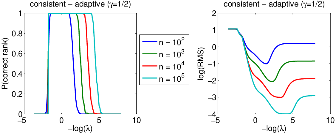
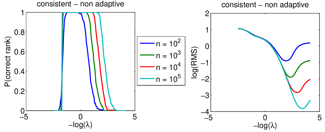
In Figure 3, we select the distribution used for the rank-consistent case of Figure 2, and compute the paths from 200 replications for n=102n=10^{2}, 10310^{3}, 10310^{3} and 10510^{5}. For each λ\lambda, we plot the proportion of estimates with correct rank on the left plots (i.e., we get an estimation of ℙ⁡(rank(W^)=rank(𝐖)){\mathbb{P}}(\mathop{\rm rank}(\hat{W})=\mathop{\rm rank}(\mathbf{W})), while we plot the logarithm of the average root mean squared estimation error ‖W^−𝐖‖\|\hat{W}-\mathbf{W}\| on the right plot. For the three regularization schemes, the range of values with high probability of correct rank selection increases as nn increases, and, most importantly achieves good mean squared error (right plot); in particular, for the non adaptive schemes (top plots), this corroborates the results from Proposition 9, which states that for λn=λ0n−1/2\lambda_{n}=\lambda_{0}n^{-1/2} the probability tends to a limit in (0,1)(0,1): indeed, when nn increases, the value λn\lambda_{n} which achieves a particular limit grows as n−1/2n^{-1/2}, and considering the log-scale for λn\lambda_{n} in Figure 3 and the uniform sampling for nn in log-scale as well, the regular spacing between the decaying parts observed in Figure 3 is coherent with our results.
Refer to caption
Refer to caption
Refer to caption
Figure 3: Synthetic example where consistency condition in Eq. (8) is satisfied: probability of correct rank selection (left) and logarithm of the expected mean squared estimation error (right), for several number of samples as a function of the regularization parameter, for regular regularization (top), adaptive regularization with γ=1/2\gamma=1/2 (center) and γ=1\gamma=1 (bottom).

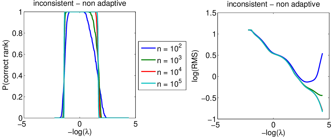
In Figure 4, we perform the same operations but with the inconsistent case of Figure 2. For the non adaptive case (top plot), the range of values of λ\lambda that achieve high probability of correct rank selection does not increase when nn increases and stays bounded, in places where the estimation error is not tending to zero: in the inconsistent case, the trace norm regularization does not manage to solve the trade-off between rank consistency and regular consistency. However, for the adaptive versions, it does, still with a somewhat singular behavior of the limiting case γ=1\gamma=1.

Refer to caption
Refer to caption
Refer to caption
Figure 4: Synthetic example where consistency condition in Eq. (7) is not satisfied: probability of correct rank selection (left) and logarithm of the expected mean squared estimation error (right), for several number of samples as a function of the regularization parameter, for regular regularization (top), adaptive regularization with γ=1/2\gamma=1/2 (center) and γ=1\gamma=1 (bottom).

Finally, in Figure 5, we consider 400 different distributions with various values of ‖Λ‖\|\Lambda\| smaller or greater than one, and computed the regularization paths with n=103n=10^{3} samples. From the paths, we consider the estimate W^\hat{W} with correct rank and best distance to 𝐖\mathbf{W} and plot the best error versus log10⁡(‖Λ‖2)\log_{10}(\|\Lambda\|_{2}). For positive values of log10⁡(‖Λ‖2)\log_{10}(\|\Lambda\|_{2}), the best error is far from zero, and the error grows with the distance to zero; while for negative values, we get low errors with lower errors for small log10⁡(‖Λ‖2)\log_{10}(\|\Lambda\|_{2}), corroborating the influence of ‖λ‖2\|\lambda\|_{2} described in Proposition 9.

Refer to caption
Figure 5: Scatter plots of log10⁡(‖Λ‖2)\log_{10}(\|\Lambda\|_{2}) versus the squared error of the best estimate with correct rank (i.e., such that rank(W^)=𝐫\mathop{\rm rank}(\hat{W})=\mathbf{r} and ‖W^−𝐖‖\|\hat{W}-\mathbf{W}\| as small as possible). See text for details.

7 Conclusion

We have presented an analysis of the rank consistency for the penalization by the trace norm, and derived general necessary and sufficient conditions. This work can be extended in several interesting ways: first, by going from the square loss to more general losses, in particular for other types of supervised learning problems such as classification; or by looking at the collaborative filtering setting where only some of the attributes are observed (Abernethy et al. 2006) and dimensions pp and qq are allowed to grow. Moreover, we are currently pursuing non asymptotic extensions of the current work, making links with the recent work of Recht et al. 2007 and of Meinshausen and Yu 2006.

Appendix A Tools for analysis of singular value decomposition

In this appendix, we review and derive precise results regarding singular value decompositions. We consider W∈ℝp×qW\in\mathbb{R}^{p\times q} and we let denote W=U​Diag(s)​V⊤W=U\mathop{\rm Diag}(s)V^{\top} its singular value decomposition with U∈ℝp×rU\in\mathbb{R}^{p\times r}, V∈ℝq×rV\in\mathbb{R}^{q\times r} with orthonormal columns, and s∈ℝrs\in\mathbb{R}^{r} with strictly positive values (rr is the rank of WW). Note that when a singular value sis_{i} is simple, i.e., does not coalesce with any other singular values, then the vectors uiu_{i} and viv_{i} are uniquely defined up to simultaneous sign flips, i.e., only the matrix ui​vi⊤u_{i}v_{i}^{\top} is unique. However, when some singular values coalesce, then the corresponding singular vectors are defined up to a rotation, and thus in general care must be taken and considering isolated singular vectors should be avoided (Stewart and Sun 1990). All tools presented in this appendix are robust to the particular choice of the singular vectors.

A.1 Jordan-Wielandt matrix

We use the fact that singular values of WW can be obtained from the eigenvalues of the Jordan-Wielandt matrix W¯=(0WW⊤0)∈ℝ(p+q)×(p+q)\bar{W}=\left(\begin{array}[]{cc}0&W\\ W^{\top}&0\end{array}\right)\in\mathbb{R}^{(p+q)\times(p+q)} (Stewart and Sun 1990). Indeed this matrix has eigenvalues sis_{i} and −si-s_{i}, i=1,…,ri=1,\dots,r, where sis_{i} are the (strictly positive) singular values of WW, with eigenvectors 12​(uivi)\frac{1}{\sqrt{2}}\left(\begin{array}[]{c}u_{i}\\ v_{i}\end{array}\right) and 12​(ui−vi)\frac{1}{\sqrt{2}}\left(\begin{array}[]{c}u_{i}\\ -v_{i}\end{array}\right) where ui,viu_{i},v_{i} are the left and right associated singular vectors. Also, the remaining eigenvalues are all equal to zero, with eigensubspace (of dimension p+q−2​rp+q-2r) composed of all (uv)\left(\begin{array}[]{c}u\\ v\end{array}\right) such that for all i∈{1,…,r}i\in\{1,\dots,r\}, u⊤​ui=v⊤​vi=0u^{\top}u_{i}=v^{\top}v_{i}=0. We let denote U¯\bar{U} the eigenvectors of W¯\bar{W} corresponding to non zero eigenvalues in S¯\bar{S}. We have U¯=12​(UUV−V)\bar{U}=\frac{1}{\sqrt{2}}\left(\begin{array}[]{cc}U&U\\ V&-V\end{array}\right) and S¯=12​(Diag(s)00−Diag(s))\bar{S}=\frac{1}{\sqrt{2}}\left(\begin{array}[]{cc}\mathop{\rm Diag}(s)&0\\ 0&-\mathop{\rm Diag}(s)\end{array}\right) and W¯=U¯​S¯​U¯⊤\bar{W}=\bar{U}\bar{S}\bar{U}^{\top}, U¯​U¯⊤=(U​U⊤00V​V⊤)\bar{U}\bar{U}^{\top}=\left(\begin{array}[]{cc}UU^{\top}&0\\ 0&VV^{\top}\end{array}\right), and U¯​sign​(S¯)​U¯⊤=(0U​V⊤V​U⊤0)\bar{U}{\rm sign}(\bar{S})\bar{U}^{\top}=\left(\begin{array}[]{cc}0&UV^{\top}\\ VU^{\top}&0\end{array}\right).

A.2 Cauchy residue formula and eigenvalues

Given the matrix W¯\bar{W}, and a simple closed curve 𝒞\mathcal{C} in the complex plane that does not go through any of the eigenvalues of W¯\bar{W}, then

Π𝒞​(W¯)=12​i​π​∮𝒞d​λλ​𝐈−W¯\Pi_{\mathcal{C}}(\bar{W})=\frac{1}{2i\pi}\oint_{\mathcal{C}}\frac{d\lambda}{\lambda\mathbf{I}-\bar{W}}

is equal to the orthogonal projection onto the orthogonal sum of all eigensubspaces of W¯\bar{W} associated with eigenvalues in the interior of 𝒞\mathcal{C} (Kato 1966). This is easily seen by writing down the eigenvalue decomposition and the Cauchy residue formula (12​i​π​∮𝒞d​λλ−λi=1\frac{1}{2i\pi}\oint_{\mathcal{C}}\frac{d\lambda}{\lambda-\lambda_{i}}=1 if λi\lambda_{i} is in the interior int⁡(𝒞){\rm int}(\mathcal{C}) of 𝒞\mathcal{C} and 00 otherwise), and:

12​i​π∮𝒞d​λλ​𝐈−W¯=∑i=12​ru¯iu¯i⊤×12​i​π∮𝒞d​λλ−s¯i=∑i,s¯i∈int⁡(𝒞)uiui⊤.\frac{1}{2i\pi}\oint_{\mathcal{C}}\frac{d\lambda}{\lambda\mathbf{I}-\bar{W}}=\sum_{i=1}^{2r}\bar{u}_{i}\bar{u}_{i}^{\top}\times\frac{1}{2i\pi}\oint_{\mathcal{C}}\frac{d\lambda}{\lambda-\bar{s}_{i}}=\sum_{i,\ \bar{s}_{i}\in{\rm int}(\mathcal{C})}u_{i}u_{i}^{\top}.

See Rudin 1987 for an introduction to complex analysis and Cauchy residue formula. Moreover, we can obtain the restriction of W¯\bar{W} onto a specific eigensubspace as:

W¯Π𝒞(W¯)=12​i​π∮𝒞W¯​d​λλ​𝐈−W¯=−12​i​π∮𝒞λ​d​λλ​𝐈−W¯.\bar{W}\Pi_{\mathcal{C}}(\bar{W})=\frac{1}{2i\pi}\oint_{\mathcal{C}}\frac{\bar{W}d\lambda}{\lambda\mathbf{I}-\bar{W}}=-\frac{1}{2i\pi}\oint_{\mathcal{C}}\frac{\lambda d\lambda}{\lambda\mathbf{I}-\bar{W}}.

We let denote s1s_{1} and srs_{r} the largest and smallest strictly positive singular values of WW; if ‖Δ‖2<sr/2\|\Delta\|_{2}<s_{r}/2, then W+ΔW+\Delta has rr singular values strictly greater than sr/2s_{r}/2 and the remaining ones are strictly less than sr/2s_{r}/2 (Stewart and Sun 1990). Thus, if we denote 𝒞\mathcal{C} the oriented circle of radius sr/2s_{r}/2, Π𝒞​(W¯)\Pi_{\mathcal{C}}(\bar{W}) is the projector on the p+q−2​rp+q-2r-dimensional null space of W¯\bar{W}, and for any Δ\Delta such that ‖Δ‖2<sr/2\|\Delta\|_{2}<s_{r}/2, Π𝒞​(W¯+Δ¯)\Pi_{\mathcal{C}}(\bar{W}+\bar{\Delta}) is also the projector on the p+q−2​rp+q-2r-dimensional invariant subspace of W¯+Δ¯\bar{W}+\bar{\Delta}, which corresponds to the smallest eigenvalues. We let denote Πo​(W¯+Δ¯)\Pi_{o}(\bar{W}+\bar{\Delta}) that projector and Πr​(W¯+Δ¯)=𝐈−Πo​(W¯+Δ¯)\Pi_{r}(\bar{W}+\bar{\Delta})=\mathbf{I}-\Pi_{o}(\bar{W}+\bar{\Delta}) the orthogonal projector (which is the projection onto the 2​r2r-th principal subspace).

We can now find expansions around Δ=0\Delta=0 as follows:

Πo​(W¯+Δ¯)−Πo​(W¯)\displaystyle\Pi_{o}(\bar{W}+\bar{\Delta})-\Pi_{o}(\bar{W}) =\displaystyle= 12​i​π​∮𝒞(λ​𝐈−W¯)−1​Δ¯​(λ​𝐈−W¯−Δ¯)−1​𝑑λ\displaystyle\frac{1}{2i\pi}\oint_{\mathcal{C}}(\lambda\mathbf{I}-\bar{W})^{-1}\bar{\Delta}(\lambda\mathbf{I}-\bar{W}-\bar{\Delta})^{-1}d\lambda
=\displaystyle= 12​i​π​∮𝒞(λ​𝐈−W¯)−1​Δ¯​(λ​𝐈−W¯)−1​𝑑λ\displaystyle\frac{1}{2i\pi}\oint_{\mathcal{C}}(\lambda\mathbf{I}-\bar{W})^{-1}\bar{\Delta}(\lambda\mathbf{I}-\bar{W})^{-1}d\lambda
+12​i​π∮𝒞(λ𝐈−W¯)−1Δ¯(λ𝐈−W¯)−1Δ¯(λ𝐈−W¯−Δ¯)−1dλ,\displaystyle+\frac{1}{2i\pi}\oint_{\mathcal{C}}(\lambda\mathbf{I}-\bar{W})^{-1}\bar{\Delta}(\lambda\mathbf{I}-\bar{W})^{-1}\bar{\Delta}(\lambda\mathbf{I}-\bar{W}-\bar{\Delta})^{-1}d\lambda,

and

(W¯+Δ¯)​Πo​(W¯+Δ¯)−W¯​Πo​(W¯)\displaystyle(\bar{W}+\bar{\Delta})\Pi_{o}(\bar{W}+\bar{\Delta})\!-\!\bar{W}\Pi_{o}(\bar{W})\!\!\!\! =\displaystyle= −12​i​π∮𝒞λ(λ𝐈−W¯)−1Δ¯(λ𝐈−W¯−Δ¯)−1dλ\displaystyle-\frac{1}{2i\pi}\oint_{\mathcal{C}}\lambda(\lambda\mathbf{I}-\bar{W})^{-1}\bar{\Delta}(\lambda\mathbf{I}-\bar{W}-\bar{\Delta})^{-1}d\lambda
=\displaystyle= −12​i​π∮𝒞λ(λ𝐈−W¯)−1Δ¯(λ𝐈−W¯)−1dλ\displaystyle-\frac{1}{2i\pi}\oint_{\mathcal{C}}\lambda(\lambda\mathbf{I}-\bar{W})^{-1}\bar{\Delta}(\lambda\mathbf{I}-\bar{W})^{-1}d\lambda
−12​i​π∮𝒞λ(λ𝐈−W¯)−1Δ¯(λ𝐈−W¯)−1Δ¯(λ𝐈−W¯−Δ¯)−1dλ,\displaystyle\!\!\!\!\!-\frac{1}{2i\pi}\oint_{\mathcal{C}}\lambda(\lambda\mathbf{I}-\bar{W})^{-1}\bar{\Delta}(\lambda\mathbf{I}-\bar{W})^{-1}\bar{\Delta}(\lambda\mathbf{I}-\bar{W}-\bar{\Delta})^{-1}d\lambda,

which lead to the following two propositions:

Proposition 16.

Assume WW has rank rr and ‖Δ‖2<sr/4\|\Delta\|_{2}<s_{r}/4 where srs_{r} is the smallest positive singular value of WW. Then the projection Πr​(W¯)\Pi_{r}(\bar{W}) on the first rr eigenvectors of W¯\bar{W} is such that

‖Πo​(W¯+Δ¯)−Πo​(W¯)‖2⩽4sr​‖Δ‖2\|\Pi_{o}(\bar{W}+\bar{\Delta})-\Pi_{o}(\bar{W})\|_{2}\leqslant\frac{4}{s_{r}}\|{\Delta}\|_{2}

and

‖Πo​(W¯+Δ¯)−Πo​(W¯)−(𝐈−U¯​U¯⊤)​Δ¯​U¯​S¯−1​U¯⊤−U¯​S¯−1​U¯⊤​Δ¯​(𝐈−U¯​U¯⊤)‖2⩽8sr2​‖Δ¯‖22.\|\Pi_{o}(\bar{W}+\bar{\Delta})-\Pi_{o}(\bar{W})-(\mathbf{I}-\bar{U}\bar{U}^{\top})\bar{\Delta}\bar{U}\bar{S}^{-1}\bar{U}^{\top}-\bar{U}\bar{S}^{-1}\bar{U}^{\top}\bar{\Delta}(\mathbf{I}-\bar{U}\bar{U}^{\top})\|_{2}\leqslant\frac{8}{s_{r}^{2}}\|\bar{\Delta}\|_{2}^{2}.
Proof.

For λ∈𝒞\lambda\in\mathcal{C} we have: ‖(λ​𝐈−W¯)−1‖2⩾2/sr\|(\lambda\mathbf{I}-\bar{W})^{-1}\|_{2}\geqslant 2/s_{r} and ‖(λ​𝐈−W¯−Δ¯)−1‖2⩾4/sr\|(\lambda\mathbf{I}-\bar{W}-\bar{\Delta})^{-1}\|_{2}\geqslant 4/s_{r}, which implies

‖Πr​(W¯+Δ¯)−Πr​(W¯)‖2\displaystyle\|\Pi_{r}(\bar{W}+\bar{\Delta})-\Pi_{r}(\bar{W})\|_{2} ⩽\displaystyle\leqslant 12​π​∮𝒞‖(λ​𝐈−W¯)−1‖2​‖Δ‖2​‖(λ​𝐈−W¯−Δ¯)−1‖2\displaystyle\frac{1}{2\pi}\oint_{\mathcal{C}}\|(\lambda\mathbf{I}-\bar{W})^{-1}\|_{2}\|\Delta\|_{2}\|(\lambda\mathbf{I}-\bar{W}-\bar{\Delta})^{-1}\|_{2}
⩽\displaystyle\leqslant (12​π​2​π​sr2)​‖Δ‖2​2sr​4sr.\displaystyle\left(\frac{1}{2\pi}2\pi\frac{s_{r}}{2}\right)\|\Delta\|_{2}\frac{2}{s_{r}}\frac{4}{s_{r}}.

In order to prove the other result, we simply need to compute:

12​i​π​∮𝒞(λ​𝐈−W¯)−1​Δ¯​(λ​𝐈−W¯)−1​𝑑λ\displaystyle\frac{1}{2i\pi}\oint_{\mathcal{C}}(\lambda\mathbf{I}-\bar{W})^{-1}\bar{\Delta}(\lambda\mathbf{I}-\bar{W})^{-1}d\lambda =\displaystyle= ∑i,ju¯i​u¯i⊤​Δ​u¯j​u¯j⊤​12​i​π​∮𝒞1(λ−s¯i)​(λ−s¯j)​𝑑λ\displaystyle\sum_{i,j}\bar{u}_{i}\bar{u}_{i}^{\top}\Delta\bar{u}_{j}\bar{u}_{j}^{\top}\frac{1}{2i\pi}\oint_{\mathcal{C}}\frac{1}{(\lambda-\bar{s}_{i})(\lambda-\bar{s}_{j})}d\lambda
=\displaystyle= ∑i,ju¯i​u¯i⊤​Δ​u¯j​u¯j⊤​(1i∉int⁡(𝒞)​1j∈int⁡(𝒞)s¯i+1j∉int⁡(𝒞)​1i∈int⁡(𝒞)s¯j)\displaystyle\!\!\!\sum_{i,j}\bar{u}_{i}\bar{u}_{i}^{\top}\Delta\bar{u}_{j}\bar{u}_{j}^{\top}\left(\frac{1_{i\notin{\rm int}(\mathcal{C})}1_{j\in{\rm int}(\mathcal{C})}}{\bar{s}_{i}}+\frac{1_{j\notin{\rm int}(\mathcal{C})}1_{i\in{\rm int}(\mathcal{C})}}{\bar{s}_{j}}\right)
=\displaystyle= (𝐈−U¯​U¯⊤)​Δ¯​U¯​S¯−1​U¯⊤+U¯​S¯−1​U¯⊤​Δ¯​(𝐈−U¯​U¯⊤).\displaystyle(\mathbf{I}-\bar{U}\bar{U}^{\top})\bar{\Delta}\bar{U}\bar{S}^{-1}\bar{U}^{\top}+\bar{U}\bar{S}^{-1}\bar{U}^{\top}\bar{\Delta}(\mathbf{I}-\bar{U}\bar{U}^{\top}).

∎

Proposition 17.

Assume WW has rank rr and ‖Δ‖2<sr/4\|\Delta\|_{2}<s_{r}/4 where srs_{r} is the smallest positive singular value of WW. Then the projection Πr​(W¯)\Pi_{r}(\bar{W}) on the first rr eigenvectors of W¯\bar{W} is such that

‖Πo​(W¯+Δ¯)​(W¯+Δ¯)−Πo​(W¯)​W¯‖2⩽2​‖Δ‖2\|\Pi_{o}(\bar{W}+\bar{\Delta})(\bar{W}+\bar{\Delta})-\Pi_{o}(\bar{W})\bar{W}\|_{2}\leqslant 2\|{\Delta}\|_{2}

and

‖Πo​(W¯+Δ¯)​(W¯+Δ¯)−Πo​(W¯)​W¯+(𝐈−U¯​U¯⊤)​Δ¯​(𝐈−U¯​U¯⊤)‖2⩽4sr​‖Δ¯‖22.\|\Pi_{o}(\bar{W}+\bar{\Delta})(\bar{W}+\bar{\Delta})-\Pi_{o}(\bar{W})\bar{W}+(\mathbf{I}-\bar{U}\bar{U}^{\top})\bar{\Delta}(\mathbf{I}-\bar{U}\bar{U}^{\top})\|_{2}\leqslant\frac{4}{s_{r}}\|\bar{\Delta}\|_{2}^{2}.
Proof.

For λ∈𝒞\lambda\in\mathcal{C} we have: ‖(λ​𝐈−W¯)−1‖2⩾2/sr\|(\lambda\mathbf{I}-\bar{W})^{-1}\|_{2}\geqslant 2/s_{r} and ‖(λ​𝐈−W¯−Δ¯)−1‖2⩾4/sr\|(\lambda\mathbf{I}-\bar{W}-\bar{\Delta})^{-1}\|_{2}\geqslant 4/s_{r}, which implies

‖Πr​(W¯+Δ¯)−Πr​(W¯)‖2\displaystyle\|\Pi_{r}(\bar{W}+\bar{\Delta})-\Pi_{r}(\bar{W})\|_{2} ⩽\displaystyle\leqslant 12​π​∮𝒞|λ|​‖(λ​𝐈−W¯)−1‖2​‖Δ‖2​‖(λ​𝐈−W¯−Δ¯)−1‖2\displaystyle\frac{1}{2\pi}\oint_{\mathcal{C}}|\lambda|\|(\lambda\mathbf{I}-\bar{W})^{-1}\|_{2}\|\Delta\|_{2}\|(\lambda\mathbf{I}-\bar{W}-\bar{\Delta})^{-1}\|_{2}
⩽\displaystyle\leqslant (12​π​2​π​sr2)​sr2​‖Δ‖2​2sr​4sr.\displaystyle\left(\frac{1}{2\pi}2\pi\frac{s_{r}}{2}\right)\frac{s_{r}}{2}\|\Delta\|_{2}\frac{2}{s_{r}}\frac{4}{s_{r}}.

In order to prove the other result, we simply need to compute:

−12​i​π∮𝒞λ(λ𝐈−W¯)−1Δ¯(λ𝐈−W¯)−1dλ\displaystyle-\frac{1}{2i\pi}\oint_{\mathcal{C}}\lambda(\lambda\mathbf{I}-\bar{W})^{-1}\bar{\Delta}(\lambda\mathbf{I}-\bar{W})^{-1}d\lambda =\displaystyle= −∑i,ju¯iu¯i⊤Δu¯ju¯j⊤12​i​π∮𝒞λ(λ−s¯i)​(λ−s¯j)dλ\displaystyle-\sum_{i,j}\bar{u}_{i}\bar{u}_{i}^{\top}\Delta\bar{u}_{j}\bar{u}_{j}^{\top}\frac{1}{2i\pi}\oint_{\mathcal{C}}\frac{\lambda}{(\lambda-\bar{s}_{i})(\lambda-\bar{s}_{j})}d\lambda
=\displaystyle= −∑i,ju¯iu¯i⊤Δu¯ju¯j⊤(1i∈int⁡(𝒞)1j∈int⁡(𝒞))\displaystyle\!\!\!-\sum_{i,j}\bar{u}_{i}\bar{u}_{i}^{\top}\Delta\bar{u}_{j}\bar{u}_{j}^{\top}\left(1_{i\in{\rm int}(\mathcal{C})}1_{j\in{\rm int}(\mathcal{C})}\right)
=\displaystyle= −(𝐈−U¯​U¯⊤)​Δ¯​(𝐈−U¯​U¯⊤).\displaystyle-(\mathbf{I}-\bar{U}\bar{U}^{\top})\bar{\Delta}(\mathbf{I}-\bar{U}\bar{U}^{\top}).

∎

The variations of Π⁡(W¯)\Pi(\bar{W}) translates immediately into variations of the singular projections U​U⊤UU^{\top} and V​V⊤VV^{\top}. Indeed we get that the first order variation of U​U⊤UU^{\top} is −(𝐈−U​U⊤)​Δ​V​S−1​U⊤-(\mathbf{I}-UU^{\top})\Delta VS^{-1}U^{\top} and the variation of VV is equal to −(𝐈−V​V⊤)​Δ⊤​U​S−1​V⊤-(\mathbf{I}-VV^{\top})\Delta^{\top}US^{-1}V^{\top}, with errors bounded in spectral norm by 8sr2​‖Δ‖22\frac{8}{s_{r}^{2}}\|{\Delta}\|_{2}^{2}. Similarly, when restricted to the small singular values, the first order expansion is (𝐈−U​U⊤)​Δ​(𝐈−V​V⊤)(\mathbf{I}-UU^{\top})\Delta(\mathbf{I}-VV^{\top}), with error term bounded in spectral norm by 4sr​‖Δ‖22\frac{4}{s_{r}}\|{\Delta}\|_{2}^{2}. Those results lead to the following proposition that gives a local sufficient condition for rank(W+Δ)>rank(W)\mathop{\rm rank}(W+\Delta)>\mathop{\rm rank}(W):

Proposition 18.

Assume WW has rank r<min⁡{p,q}r<\min\{p,q\} with ordered singular value decomposition W=U​Diag(s)​V⊤W=U\mathop{\rm Diag}(s)V^{\top}. If 4sr​‖Δ‖22<‖(𝐈−U​U⊤)​Δ​(𝐈−V​V⊤)‖2\frac{4}{s_{r}}\|\Delta\|_{2}^{2}<\|(\mathbf{I}-UU^{\top})\Delta(\mathbf{I}-VV^{\top})\|_{2}, then rank(W+Δ)>r\mathop{\rm rank}(W+\Delta)>r.

Appendix B Some facts about the trace norm

In this appendix, we review known properties of the trace norm that we use in this paper. Most of the results are extensions of similar results for the ℓ1\ell_{1}-norm on vectors. First, we have the following result:

Lemma 19.

(Fazel et al. 2001, Dual norm,) The trace norm ∥⋅∥∗\|\cdot\|_{\ast} is a norm and its dual norm is the operator norm ∥⋅∥\|\cdot\|.

Note that the dual norm N⁡(W)N(W) is defined as (Boyd and Vandenberghe 2003):

N⁡(W)=sup‖V‖∗⩽1tr​W⊤​V.N(W)=\sup_{\|V\|_{\ast}\leqslant 1}{\rm tr}W^{\top}V.

This immediately implies the following result:

Lemma 20.

(Fenchel conjugate) We have: maxW∈ℝp×q⁡tr​W⊤​V−‖W‖∗=0\displaystyle\max_{W\in\mathbb{R}^{p\times q}}{\rm tr}W^{\top}V-\|W\|_{\ast}=0 if ‖V‖⩽1\|V\|\leqslant 1 and +∞+\infty otherwise.

In this paper, we need to compute the subdifferential and directional derivatives of the trace norm. We have from Recht et al. 2007 or Borwein and Lewis 2000:

Proposition 21.

(Subdifferential) If W=U​Diag(s)​V⊤W=U\mathop{\rm Diag}(s)V^{\top} with U∈ℝp×mU\in\mathbb{R}^{p\times m} and V∈ℝq×mV\in\mathbb{R}^{q\times m} having orthonormal columns, and s∈ℝms\in\mathbb{R}^{m} is strictly positive, is the singular value decomposition of WW, then ‖W‖∗=∑i=1msi\|W\|_{\ast}=\sum_{i=1}^{m}s_{i} and the subdifferential of ∥⋅∥∗\|\cdot\|_{\ast} is equal to

∂∥⋅∥∗(W)={UV⊤+M, such that ∥M∥2⩽1,U⊤M=0 and MV=0}.\partial\|\cdot\|_{\ast}(W)=\left\{UV^{\top}+M,\mbox{ such that }\|M\|_{2}\leqslant 1,\ U^{\top}M=0\mbox{ and }MV=0\right\}.

This result can be extended to compute directional derivatives:

Proposition 22.

(Directional derivative) The directional derivative at W=U​S​V⊤W=USV^{\top} is equal to:

limε→0+‖W+ε​Δ‖∗−‖W‖∗ε=tr​U⊤​Δ​V+‖U⊥⊤​Δ​V⊥‖∗,\lim_{\varepsilon\to 0^{+}}\frac{\|W+\varepsilon\Delta\|_{\ast}-\|W\|_{\ast}}{\varepsilon}={\rm tr}U^{\top}\Delta V+\|U_{\bot}^{\top}\Delta V_{\bot}\|_{\ast},

where U⊥∈ℝp×(p−m)U_{\bot}\in\mathbb{R}^{p\times(p-m)} and V⊥∈ℝq×(q−m)V_{\bot}\in\mathbb{R}^{q\times(q-m)} are any orthonormal complements of UU and VV.

Proof.

From the subdifferential, we get the directional derivative (Borwein and Lewis 2000) as

limε→0+‖W+ε​Δ‖∗−‖W‖∗ε=maxV∈∂∥⋅∥∗(W)trΔ⊤V\lim_{\varepsilon\to 0^{+}}\frac{\|W+\varepsilon\Delta\|_{\ast}-\|W\|_{\ast}}{\varepsilon}=\max_{V\in\partial\|\cdot\|_{\ast}(W)}{\rm tr}\Delta^{\top}V

which exactly leads to the desired result. ∎

The final result that we use is a bit finer as it gives an upper bound on the error in the previous limit:

Proposition 23.

Let W=U​Diag(s)​V⊤W=U\mathop{\rm Diag}(s)V^{\top} the ordered singular value decomposition, where rank(W)=r\mathop{\rm rank}(W)=r, s>0s>0 and U⊥U_{\bot} and V⊥V_{\bot} be orthogonal complement of UU and VV; then, if ‖Δ‖2⩽sr/4\|\Delta\|_{2}\leqslant s_{r}/4:

|‖W+Δ‖∗−‖W‖∗−tr​U⊤​Δ​V−‖U⊥⊤​Δ​V⊥‖∗|⩽16​min⁡{p,q}​s12sr3​‖Δ‖22.\left|\|W+\Delta\|_{\ast}-\|W\|_{\ast}-{\rm tr}U^{\top}\Delta V-\|U_{\bot}^{\top}\Delta V_{\bot}\|_{\ast}\right|\leqslant 16\min\{p,q\}\frac{s_{1}^{2}}{s_{r}^{3}}\|\Delta\|_{2}^{2}.
Proof.

The trace norm of ‖W+Δ‖∗\|W+\Delta\|_{\ast} may be divided into the sum of the rr largest and the sum of the remaining singular values. The sums of the remaining ones are given through Proposition 17 by ‖U⊥⊤​Δ​V⊥‖∗\|U_{\bot}^{\top}\Delta V_{\bot}\|_{\ast} with an error bounded by min⁡{p,q}​4sr​‖Δ‖22\min\{p,q\}\frac{4}{s_{r}}\|{\Delta}\|_{2}^{2}. For the first rr singular values, we need to upperbound the second derivative of the sum of the rr largest eigenvalues of W¯+Δ¯\bar{W}+\bar{\Delta} with strictly positive eigengap, which leads to the given bound by using the same Cauchy residue technique described in Appendix A. ∎

Appendix C Proofs

C.1 Proof of Lemma 2

We let denote S∈{0,1}nx×nyS\in\{0,1\}^{n_{x}\times n_{y}} the sampling matrix; i.e., Si​j=1S_{ij}=1 if the pair (i,j)(i,j) is observed and zero otherwise. We let denote X~\tilde{X} and Y~\tilde{Y} the data matrices. We can write Mk=X~⊤​δik​δjk⊤​Y~M_{k}=\tilde{X}^{\top}\delta_{i_{k}}\delta_{j_{k}}^{\top}\tilde{Y} and:

1n​∑k=1nvec(Mk)​vec(Mk)⊤\displaystyle\frac{1}{n}\sum_{k=1}^{n}\mathop{\rm vec}(M_{k})\mathop{\rm vec}(M_{k})^{\top} =\displaystyle= 1n​∑k=1n(Y~⊗X~)⊤​vec(δik​δjk⊤)​vec(δik​δjk⊤)⊤​(Y~⊗X~)\displaystyle\frac{1}{n}\sum_{k=1}^{n}(\tilde{Y}\otimes\tilde{X})^{\top}\mathop{\rm vec}(\delta_{i_{k}}\delta_{j_{k}}^{\top})\mathop{\rm vec}(\delta_{i_{k}}\delta_{j_{k}}^{\top})^{\top}(\tilde{Y}\otimes\tilde{X})
=\displaystyle= 1n​(Y~⊗X~)⊤​Diag(vec(S))​(Y~⊗X~),\displaystyle\frac{1}{n}(\tilde{Y}\otimes\tilde{X})^{\top}\mathop{\rm Diag}(\mathop{\rm vec}(S))(\tilde{Y}\otimes\tilde{X}),

which leads to (denoting Σ^x​x=nx−1​X~⊤​X~\hat{\Sigma}_{xx}=n_{x}^{-1}\tilde{X}^{\top}\tilde{X} and Σ^y​y=nx−1​Y~⊤​Y~\hat{\Sigma}_{yy}=n_{x}^{-1}\tilde{Y}^{\top}\tilde{Y}):

(1n​∑k=1nvec(Mk)​vec(Mk)⊤−Σ^y​y⊗Σ^x​x)=1n​(Y~⊗X~)⊤​Diag(vec(S−n/nx​ny))​(Y~⊗X~).\left(\frac{1}{n}\sum_{k=1}^{n}\mathop{\rm vec}(M_{k})\mathop{\rm vec}(M_{k})^{\top}-\hat{\Sigma}_{yy}\otimes\hat{\Sigma}_{xx}\right)=\frac{1}{n}(\tilde{Y}\otimes\tilde{X})^{\top}\mathop{\rm Diag}(\mathop{\rm vec}(S-n/n_{x}n_{y}))(\tilde{Y}\otimes\tilde{X}).

We can thus compute the squared Frobenius norm:

‖1n​∑k=1nvec(Mk)​vec(Mk)⊤−Σ^y​y⊗Σ^x​x‖F2\displaystyle\left\|\frac{1}{n}\sum_{k=1}^{n}\mathop{\rm vec}(M_{k})\mathop{\rm vec}(M_{k})^{\top}-\hat{\Sigma}_{yy}\otimes\hat{\Sigma}_{xx}\right\|_{F}^{2}
=\displaystyle= 1n2​tr​Diag(vec(S−n/nx​ny))​(Y~​Y~⊤⊗X~​X~⊤)​Diag(vec(S−n/nx​ny))​(Y~​Y~⊤⊗X~​X~⊤)\displaystyle\frac{1}{n^{2}}{\rm tr}\mathop{\rm Diag}(\mathop{\rm vec}(S-n/n_{x}n_{y}))(\tilde{Y}\tilde{Y}^{\top}\otimes\tilde{X}\tilde{X}^{\top})\mathop{\rm Diag}(\mathop{\rm vec}(S-n/n_{x}n_{y}))(\tilde{Y}\tilde{Y}^{\top}\otimes\tilde{X}\tilde{X}^{\top})
=\displaystyle= 1n2​∑i,j,i′,j′(Si​j−n/nx​ny)​(Y~​Y~⊤⊗X~​X~⊤)i​j,i′​j′​(Si′​j′−n/nx​ny)​(Y~​Y~⊤⊗X~​X~⊤)i​j,i′​j′.\displaystyle\frac{1}{n^{2}}\sum_{i,j,i^{\prime},j^{\prime}}(S_{ij}-n/n_{x}n_{y})(\tilde{Y}\tilde{Y}^{\top}\otimes\tilde{X}\tilde{X}^{\top})_{ij,i^{\prime}j^{\prime}}(S_{i^{\prime}j^{\prime}}-n/n_{x}n_{y})(\tilde{Y}\tilde{Y}^{\top}\otimes\tilde{X}\tilde{X}^{\top})_{ij,i^{\prime}j^{\prime}}.

We have, by properties of sampling without replacement (Hoeffding 1963):

𝔼⁡(Si​j−n/nx​ny)​(Si′​j′−n/nx​ny)\displaystyle{\mathbb{E}}(S_{ij}-n/n_{x}n_{y})(S_{i^{\prime}j^{\prime}}-n/n_{x}n_{y}) =\displaystyle= n/nx​ny​(1−n/nx​ny)​ if ​(i,j)=(i′,j′),\displaystyle n/n_{x}n_{y}(1-n/n_{x}n_{y})\mbox{ if }(i,j)=(i^{\prime},j^{\prime}),
𝔼⁡(Si​j−n/nx​ny)​(Si′​j′−n/nx​ny)\displaystyle{\mathbb{E}}(S_{ij}-n/n_{x}n_{y})(S_{i^{\prime}j^{\prime}}-n/n_{x}n_{y}) =\displaystyle= −n/nxny(1−n/nxny)1nx​ny−1 if (i,j)≠(i′,j′).\displaystyle-n/n_{x}n_{y}(1-n/n_{x}n_{y})\frac{1}{n_{x}n_{y}-1}\mbox{ if }(i,j)\neq(i^{\prime},j^{\prime}).

This implies

𝔼⁡(‖1n​∑k=1nvec(Mk)​vec(Mk)⊤−Σ^y​y⊗Σ^x​x‖F2|X~,Y~)=1nx​ny​n​∑i,j(Y~​Y~⊤⊗X~​X~⊤)i​j,i​j2−1(nx​ny−1)​nx​ny​n​∑(i,j)≠(i′,j′)(Y~​Y~⊤⊗X~​X~⊤)i​j,i′​j′2⩽2nx​ny​n​∑i,j‖y~j‖4​‖x~i‖4.{\mathbb{E}}(\|\frac{1}{n}\sum_{k=1}^{n}\mathop{\rm vec}(M_{k})\mathop{\rm vec}(M_{k})^{\top}-\hat{\Sigma}_{yy}\otimes\hat{\Sigma}_{xx}\|_{F}^{2}|\tilde{X},\tilde{Y})\\ =\frac{1}{n_{x}n_{y}n}\sum_{i,j}(\tilde{Y}\tilde{Y}^{\top}\otimes\tilde{X}\tilde{X}^{\top})_{ij,ij}^{2}-\frac{1}{(n_{x}n_{y}-1)n_{x}n_{y}n}\sum_{(i,j)\neq(i^{\prime},j^{\prime})}(\tilde{Y}\tilde{Y}^{\top}\otimes\tilde{X}\tilde{X}^{\top})_{ij,i^{\prime}j^{\prime}}^{2}\\ \leqslant\frac{2}{n_{x}n_{y}n}\sum_{i,j}\|\tilde{y}_{j}\|^{4}\|\tilde{x}_{i}\|^{4}.

This finally implies that

𝔼​‖1n​∑k=1nvec(Mk)​vec(Mk)⊤−Σy​y⊗Σx​x‖F2\displaystyle{\mathbb{E}}\left\|\frac{1}{n}\sum_{k=1}^{n}\mathop{\rm vec}(M_{k})\mathop{\rm vec}(M_{k})^{\top}-\Sigma_{yy}\otimes\Sigma_{xx}\right\|_{F}^{2}
⩽\displaystyle\leqslant 4n​∑i,j𝔼​‖x‖4​𝔼​‖y‖4+2​𝔼​‖Σ^x​x−Σx​x‖F2​𝔼​‖Σ^y​y‖F2+2​𝔼​‖Σ^y​y−Σy​y‖F2​‖Σx​x‖F2\displaystyle\frac{4}{n}\sum_{i,j}{\mathbb{E}}\|x\|^{4}{\mathbb{E}}\|y\|^{4}+2{\mathbb{E}}\|\hat{\Sigma}_{xx}-\Sigma_{xx}\|_{F}^{2}{\mathbb{E}}\|\hat{\Sigma}_{yy}\|_{F}^{2}+2{\mathbb{E}}\|\hat{\Sigma}_{yy}-\Sigma_{yy}\|_{F}^{2}\|\Sigma_{xx}\|_{F}^{2}
⩽\displaystyle\leqslant C​𝔼​‖x‖4​𝔼​‖y‖4×(1n+1ny+1nx),\displaystyle C{\mathbb{E}}\|x\|^{4}{\mathbb{E}}\|y\|^{4}\times(\frac{1}{n}+\frac{1}{n_{y}}+\frac{1}{n_{x}}),

for some constant C>0C>0. This implies (A(A2)). To prove the asymptotic normality in (A(A3)), we use the martingale central limit theorem (Hall and Heyde 1980) with sequence of σ\sigma-fields ℱn,k=σ⁡(X~,Y~,ε1,…,εk,(i1,j1),…,(ik,jk))\mathcal{F}_{n,k}=\sigma(\tilde{X},\tilde{Y},\varepsilon_{1},\dots,\varepsilon_{k},(i_{1},j_{1}),\dots,(i_{k},j_{k})) for k⩽nk\leqslant n. We consider Δn,k=n−1/2εik​jkyjk⊗xik∈ℝp​q\Delta_{n,k}=n^{-1/2}\varepsilon_{i_{k}j_{k}}y_{j_{k}}\otimes x_{i_{k}}\in\mathbb{R}^{pq} as the martingale difference. We have 𝔼⁡(Δn,k|ℱn,k−1)=0{\mathbb{E}}(\Delta_{n,k}|\mathcal{F}_{n,k-1})=0 and

𝔼⁡(Δn,k​Δn,k⊤|ℱn,k−1)=n−1​σ2​yjk​yjk⊤⊗xik​xik⊤,{\mathbb{E}}(\Delta_{n,k}\Delta_{n,k}^{\top}|\mathcal{F}_{n,k-1})=n^{-1}\sigma^{2}y_{j_{k}}y_{j_{k}}^{\top}\otimes x_{i_{k}}x_{i_{k}}^{\top},

with 𝔼(∥Δn,k)∥4)=O(n−2){\mathbb{E}}(\|\Delta_{n,k})\|^{4})=O(n^{-2}) because of the finite fourth order moments. Moreover,

∑k=1n𝔼⁡(Δn,k​Δn,k⊤|ℱn,k−1)=σ2​Σ^m​m,\sum_{k=1}^{n}{\mathbb{E}}(\Delta_{n,k}\Delta_{n,k}^{\top}|\mathcal{F}_{n,k-1})=\sigma^{2}\hat{\Sigma}_{mm},

and thus tends in probability to σ2​Σy​y⊗Σx​x\sigma^{2}\Sigma_{yy}\otimes\Sigma_{xx} because of (A(A2)). The assumptions of the martingale central limit theorem are met, we have that ∑k=1nvec(Δn,k)\sum_{k=1}^{n}\mathop{\rm vec}(\Delta_{n,k}) is asymptotically normal with mean zero and covariance matrix σ2​Σy​y⊗Σx​x\sigma^{2}\Sigma_{yy}\otimes\Sigma_{xx}, which concludes the proof.

C.2 Proof of Proposition 4

We may first restrict minimization over the ball {W,‖W‖∗⩽‖Σ^m​m−1​Σ^M​z‖∗}\{W,\ \|W\|_{\ast}\leqslant\|\hat{\Sigma}_{mm}^{-1}\hat{\Sigma}_{Mz}\|_{\ast}\} because the optimum value is less than the value for W=Σ^m​m−1​Σ^M​zW=\hat{\Sigma}_{mm}^{-1}\hat{\Sigma}_{Mz}. Since this random variable is bounded in probability, we can reduce the problem to a compact set. The sequence of continuous random functions W↦12​vec(W−𝐖)⊤​Σ^m​m​vec(W−𝐖)−tr​W⊤​Σ^M​ε+λn​‖W‖∗W\mapsto\frac{1}{2}\mathop{\rm vec}(W-\mathbf{W})^{\top}\hat{\Sigma}_{mm}\mathop{\rm vec}(W-\mathbf{W})-{\rm tr}W^{\top}\hat{\Sigma}_{M\varepsilon}+\lambda_{n}\|W\|_{\ast} converges pointwise in probability to W↦12​vec(W−𝐖)⊤​Σm​m​vec(W−𝐖)+λ0​‖W‖∗W\mapsto\frac{1}{2}\mathop{\rm vec}(W-\mathbf{W})^{\top}\Sigma_{mm}\mathop{\rm vec}(W-\mathbf{W})+\lambda_{0}\|W\|_{\ast} with a unique global minimum (because Σm​m\Sigma_{mm} is assumed invertible). We can thus apply standard result of consistency in M-estimation (Van der Vaart 1998; Shao 2003).

C.3 Proof of Proposition 7

We consider the result of Proposition 6: Δ^=n1/2​(W^−𝐖)\hat{\Delta}=n^{1/2}(\hat{W}-\mathbf{W}) is asymptotically normal with mean zero and covariance σ2​Σm​m−1\sigma^{2}\Sigma_{mm}^{-1}. By Proposition 18 in Appendix B, if 4n−1/2sr​‖Δ^‖22<‖𝐔⊥⊤​Δ^​𝐕⊥‖2\frac{4n^{-1/2}}{s_{r}}\|\hat{\Delta}\|_{2}^{2}<\|\mathbf{U}_{\bot}^{\top}\hat{\Delta}\mathbf{V}_{\bot}\|_{2}, then rank(W^)>𝐫\mathop{\rm rank}(\hat{W})>\mathbf{r}. For a random variable Θ\Theta with normal distribution with mean zero and covariance matrix σ2​Σm​m−1\sigma^{2}\Sigma_{mm}^{-1}, we let denote f⁡(C)=ℙ⁡(4C−1/2sr​‖Θ‖22<‖𝐔⊥⊤​Θ​𝐕⊥‖2)f(C)={\mathbb{P}}(\frac{4C^{-1/2}}{s_{r}}\|\Theta\|_{2}^{2}<\|\mathbf{U}_{\bot}^{\top}\Theta\mathbf{V}_{\bot}\|_{2}). By the dominated convergence theorem, f⁡(C)f(C) converges to one when C→∞C\to\infty. Let ε>0\varepsilon>0, thus there exists C0>0C_{0}>0 such that f⁡(C0)>1−ε/2f(C_{0})>1-\varepsilon/2. By the asymptotic normality result, ℙ⁡(4C0−1/2sr​‖Δ^‖22<‖𝐔⊥⊤​Δ^​𝐕⊥‖2){\mathbb{P}}(\frac{4C_{0}^{-1/2}}{s_{r}}\|\hat{\Delta}\|_{2}^{2}<\|\mathbf{U}_{\bot}^{\top}\hat{\Delta}\mathbf{V}_{\bot}\|_{2}) converges to f⁡(C0)f(C_{0}) thus ∃n0>0\exists n_{0}>0 such that ∀n>n0\forall n>n_{0}, ℙ⁡(4C0−1/2sr​‖Δ^‖22<‖𝐔⊥⊤​Δ^​𝐕⊥‖2)>f⁡(C0)−ε/2>1−ε{\mathbb{P}}(\frac{4C_{0}^{-1/2}}{s_{r}}\|\hat{\Delta}\|_{2}^{2}<\|\mathbf{U}_{\bot}^{\top}\hat{\Delta}\mathbf{V}_{\bot}\|_{2})>f(C_{0})-\varepsilon/2>1-\varepsilon, which concludes the proof, because ℙ⁡(4n−1/2sr​‖Δ^‖22<‖𝐔⊥⊤​Δ^​𝐕⊥‖2)⩾ℙ⁡(4C0−1/2sr​‖Δ^‖22<‖𝐔⊥⊤​Δ^​𝐕⊥‖2){\mathbb{P}}(\frac{4n^{-1/2}}{s_{r}}\|\hat{\Delta}\|_{2}^{2}<\|\mathbf{U}_{\bot}^{\top}\hat{\Delta}\mathbf{V}_{\bot}\|_{2})\geqslant{\mathbb{P}}(\frac{4C_{0}^{-1/2}}{s_{r}}\|\hat{\Delta}\|_{2}^{2}<\|\mathbf{U}_{\bot}^{\top}\hat{\Delta}\mathbf{V}_{\bot}\|_{2}) as soon as n>C0n>C_{0}.

C.4 Proof of Proposition 8

This is the same result as Fu and Knight 2000, but extended to the trace norm minimization, simply using the directional derivative result of Proposition 22 and the epiconvergence theorem from Geyer 1994; Geyer 1996. Indeed, if we denote Vn(Δ)=vec(Δ)⊤Σ^m​mvec(Δ)−trΔ⊤n1/2Σ^M​ε+λ0n1/2(∥𝐖+n−1/2Δ∥∗−∥𝐖∥∗)V_{n}(\Delta)=\mathop{\rm vec}(\Delta)^{\top}\hat{\Sigma}_{mm}\mathop{\rm vec}(\Delta)-{\rm tr}\Delta^{\top}n^{1/2}\hat{\Sigma}_{M\varepsilon}+\lambda_{0}n^{1/2}(\|\mathbf{W}+n^{-1/2}\Delta\|_{\ast}-\|\mathbf{W}\|_{\ast}) and V⁡(Δ)=vec(Δ)⊤​Σm​m​vec(Δ)−tr​Δ⊤​A+λ0​[tr​𝐔⊤​Δ​𝐕+‖𝐔⊥⊤​Δ​𝐕⊥‖∗]V(\Delta)=\mathop{\rm vec}(\Delta)^{\top}\Sigma_{mm}\mathop{\rm vec}(\Delta)-{\rm tr}\Delta^{\top}A+\lambda_{0}\left[{\rm tr}\mathbf{U}^{\top}\Delta\mathbf{V}+\|\mathbf{U}_{\bot}^{\top}\Delta\mathbf{V}_{\bot}\|_{\ast}\right], then for each Δ\Delta, Vn​(Δ)V_{n}(\Delta) converges in probability to V⁡(Δ)V(\Delta), and VV is strictly convex, which implies that it has an unique global minimum; thus the epi-convergence theorem can be applied, which concludes the proof.

Note that a simpler analysis using regular tools in M-estimation leads to W^=𝐖+n−1/2Δ^+op(n−1/2)\hat{W}=\mathbf{W}+n^{-1/2}\hat{\Delta}+o_{p}(n^{-1/2}), where Δ^\hat{\Delta} is the unique global minimizer of

minΔ∈ℝp×q⁡12​vec(Δ)⊤​Σm​m​vec(Δ)−tr​Δ⊤​(n1/2​Σ^M​ε)+λ0​[tr​𝐔⊤​Δ​𝐕+‖𝐔⊥⊤​Δ​𝐕⊥‖∗],\min_{\Delta\in\mathbb{R}^{p\times q}}\frac{1}{2}\mathop{\rm vec}(\Delta)^{\top}\Sigma_{mm}\mathop{\rm vec}(\Delta)-{\rm tr}\Delta^{\top}(n^{1/2}\hat{\Sigma}_{M\varepsilon})+\lambda_{0}\left[{\rm tr}\mathbf{U}^{\top}\Delta\mathbf{V}+\|\mathbf{U}_{\bot}^{\top}\Delta\mathbf{V}_{\bot}\|_{\ast}\right],

i.e., we can actually take A=n1/2​Σ^M​εA=n^{1/2}\hat{\Sigma}_{M\varepsilon} (which is asymptotically normal with correct moments).

C.5 Proof of Proposition 9

We let denote Δ^=n1/2​(W^−𝐖)\hat{\Delta}=n^{1/2}(\hat{W}-\mathbf{W}). We first show that limsupn→∞ℙ⁡(rank(W^)=𝐫)\lim\sup_{n\to\infty}{\mathbb{P}}(\mathop{\rm rank}(\hat{W})=\mathbf{r}) is smaller than the proposed limit aa. We consider the following events:

E0\displaystyle E_{0} =\displaystyle= {rank(W^)=𝐫}\displaystyle\{\mathop{\rm rank}(\hat{W})=\mathbf{r}\}
E1\displaystyle E_{1} =\displaystyle= {∥n−1/2Δ^∥2<𝐬r/2}\displaystyle\{\|n^{-1/2}\hat{\Delta}\|_{2}<\mathbf{s}_{r}/2\}
E2\displaystyle E_{2} =\displaystyle= {4n−1/2sr∥Δ^∥22<∥𝐔⊥⊤Δ^𝐕⊥∥2}.\displaystyle\left\{\frac{4n^{-1/2}}{s_{r}}\|\hat{\Delta}\|_{2}^{2}<\|\mathbf{U}_{\bot}^{\top}\hat{\Delta}\mathbf{V}_{\bot}\|_{2}\right\}.

By Proposition 18 in Appendix B, we have E1∩E2⊂E0cE_{1}\cap E_{2}\subset E_{0}^{c}, and thus it suffices to show that ℙ⁡(E1){\mathbb{P}}(E_{1}) tends to one, while limsupn→∞ℙ⁡(E2c)⩽a\lim\sup_{n\to\infty}{\mathbb{P}}(E_{2}^{c})\leqslant a. The first assertion is a simple consequence of Proposition 8.

Moreover, by Proposition 8, Δ^\hat{\Delta} converges in distribution to the unique global optimum Δ⁡(A)\Delta(A) of an optimization problem parameterized by a vector AA with normal distribution. For a given η>0\eta>0, we consider the probability ℙ⁡(‖𝐔⊥⊤​Δ​(A)​𝐕⊥‖2⩽η){\mathbb{P}}(\|\mathbf{U}_{\bot}^{\top}\Delta(A)\mathbf{V}_{\bot}\|_{2}\leqslant\eta). For any AA, when η\eta tends to zero, the indicator function 1‖𝐔⊥⊤​Δ​(A)​𝐕⊥‖2⩽η1_{\|\mathbf{U}_{\bot}^{\top}\Delta(A)\mathbf{V}_{\bot}\|_{2}\leqslant\eta} converges to 1‖𝐔⊥⊤​Δ​(A)​𝐕⊥‖2=01_{\|\mathbf{U}_{\bot}^{\top}\Delta(A)\mathbf{V}_{\bot}\|_{2}=0}, which is equal to 1‖Λ⁡(A)‖2⩽λ01_{\|\Lambda(A)\|_{2}\leqslant\lambda_{0}}, where

vec(Λ⁡(A))=((𝐕⊥⊗𝐔⊥)⊤​Σm​m−1​(𝐕⊥⊗𝐔⊥))−1​((𝐕⊥⊗𝐔⊥)⊤​Σm​m−1​((𝐕⊗𝐔)​vec(𝐈)−vec(A))).\mathop{\rm vec}(\Lambda(A))=\left((\mathbf{V}_{\bot}\otimes\mathbf{U}_{\bot})^{\top}\Sigma_{mm}^{-1}(\mathbf{V}_{\bot}\otimes\mathbf{U}_{\bot})\right)^{-1}\!\!\left((\mathbf{V}_{\bot}\otimes\mathbf{U}_{\bot})^{\top}\Sigma_{mm}^{-1}((\mathbf{V}\otimes\mathbf{U})\mathop{\rm vec}(\mathbf{I})\!-\!\mathop{\rm vec}(A))\right).

By the dominated convergence theorem, ℙ⁡(‖𝐔⊥⊤​Δ​(A)​𝐕⊥‖2⩽η){\mathbb{P}}(\|\mathbf{U}_{\bot}^{\top}\Delta(A)\mathbf{V}_{\bot}\|_{2}\leqslant\eta) converges to a=ℙ⁡(‖Λ⁡(A)‖2⩽λ0)a={\mathbb{P}}(\|\Lambda(A)\|_{2}\leqslant\lambda_{0}), which is the proposed limit. This limit is in (0,1)(0,1) because of the normal distribution has an invertible covariance matrix and the set {∥Λ∥2⩽1}\{\|\Lambda\|_{2}\leqslant 1\} and its complement have non empty interiors.

Since Δ^=Op​(1)\hat{\Delta}=O_{p}(1), we can instead consider E3={4n−1/2srM2<∥𝐔⊥⊤Δ^𝐕⊥∥2}E_{3}=\{\frac{4n^{-1/2}}{s_{r}}M^{2}<\|\mathbf{U}_{\bot}^{\top}\hat{\Delta}\mathbf{V}_{\bot}\|_{2}\} for a particular MM, instead of E2E_{2}. Then following the same line or arguments than in Appendix C.3, we conclude that limsupn→∞ℙ⁡(E3c)⩽a\lim\sup_{n\to\infty}{\mathbb{P}}(E_{3}^{c})\leqslant a, which concludes the first part of the proof.

We now show that liminfn→∞ℙ⁡(rank(W^)=𝐫)⩾a\lim\inf_{n\to\infty}{\mathbb{P}}(\mathop{\rm rank}(\hat{W})=\mathbf{r})\geqslant a. A sufficient condition for rank consistency is the following: we let denote W^=U​S​V⊤\hat{W}=USV^{\top} the singular value decomposition of W^\hat{W} and we let denote UoU_{o} and VoV_{o} the singular vectors corresponding to all but the 𝐫\mathbf{r} largest singular values. Since we have simultaneous singular value decompositions, a sufficient condition is that rank(W^)⩾𝐫\mathop{\rm rank}(\hat{W})\geqslant\mathbf{r} and ‖Uo⊤​(Σ^m​m​(W^−𝐖)−Σ^M​ε)​Vo‖2<λn​(1−η)\left\|U_{o}^{\top}\left(\hat{\Sigma}_{mm}(\hat{W}-\mathbf{W})-\hat{\Sigma}_{M\varepsilon}\right)V_{o}\right\|_{2}<\lambda_{n}(1-\eta). If ‖Λ⁡(n1/2​Σ^M​ε)‖⩽λ0​(1−η)\|\Lambda(n^{1/2}\hat{\Sigma}_{M\varepsilon})\|\leqslant\lambda_{0}(1-\eta), then, by Lemma 11, 𝐔⊥⊤​Δ​(n1/2​Σ^M​ε)​𝐕⊥=0\mathbf{U}_{\bot}^{\top}\Delta(n^{1/2}\hat{\Sigma}_{M\varepsilon})\mathbf{V}_{\bot}=0, and we get, using the proof of Proposition 8 and the notation A^=n1/2​Σ^M​ε\hat{A}=n^{1/2}\hat{\Sigma}_{M\varepsilon}:

Uo⊤​(Σ^m​m​(W^−𝐖)−Σ^M​ε)​Vo\displaystyle U_{o}^{\top}\left(\hat{\Sigma}_{mm}(\hat{W}-\mathbf{W})-\hat{\Sigma}_{M\varepsilon}\right)V_{o} =\displaystyle= Uo⊤n−1/2(Σ^m​mΔ(A^)−A^)Vo+op(n−1/2).\displaystyle U_{o}^{\top}n^{-1/2}\left(\hat{\Sigma}_{mm}\Delta(\hat{A})-\hat{A}\right)V_{o}+o_{p}(n^{-1/2}).

Moreover, because of regular consistency and a positive eigengap for 𝐖\mathbf{W}, the projection onto the first 𝐫\mathbf{r} singular vectors of W^\hat{W} converges to the projection onto the first 𝐫\mathbf{r} singular vectors of 𝐖\mathbf{W} (see Appendix A), which implies that the projection onto the orthogonal is also consistent, i.e., Uo​Uo⊤U_{o}U_{o}^{\top} converges in probability to 𝐔⊥​𝐔⊥⊤\mathbf{U}_{\bot}\mathbf{U}_{\bot}^{\top} and Vo​Vo⊤V_{o}V_{o}^{\top} converges in probability to 𝐕⊥​𝐕⊥⊤\mathbf{V}_{\bot}\mathbf{V}_{\bot}^{\top}. Thus:

‖Uo⊤​(Σ^m​m​(W^−𝐖)−Σ^M​ε)​Vo‖2\displaystyle\left\|U_{o}^{\top}\left(\hat{\Sigma}_{mm}(\hat{W}-\mathbf{W})-\hat{\Sigma}_{M\varepsilon}\right)V_{o}\right\|_{2} =\displaystyle= ‖Uo​Uo⊤​(Σ^m​m​(W^−𝐖)−Σ^M​ε)​Vo​Vo⊤‖2\displaystyle\left\|U_{o}U_{o}^{\top}\left(\hat{\Sigma}_{mm}(\hat{W}-\mathbf{W})-\hat{\Sigma}_{M\varepsilon}\right)V_{o}V_{o}^{\top}\right\|_{2}
=\displaystyle= Än−1/2∥𝐔⊥𝐔⊥⊤(Σ^m​mΔ(A^)−A^)𝐕⊥𝐕⊥⊤∥2+op(n−1/2)\displaystyle Än^{-1/2}\|\mathbf{U}_{\bot}\mathbf{U}_{\bot}^{\top}(\hat{\Sigma}_{mm}\Delta(\hat{A})-\hat{A})\mathbf{V}_{\bot}\mathbf{V}_{\bot}^{\top}\|_{2}+o_{p}(n^{-1/2})
=\displaystyle= n−1/2∥Λ(A)∥2+op(n−1/2).\displaystyle n^{-1/2}\|\Lambda(A)\|_{2}+o_{p}(n^{-1/2}).

This implies that

liminfn→∞‖Uo⊤​(Σ^m​m​(W^−𝐖)−Σ^M​ε)​Vo‖2<λn​(1−η)⩾liminfn→∞ℙ⁡(‖Λ⁡(A^)‖2⩽λ0​(1−η))\lim\inf_{n\to\infty}\left\|U_{o}^{\top}\left(\hat{\Sigma}_{mm}(\hat{W}-\mathbf{W})-\hat{\Sigma}_{M\varepsilon}\right)V_{o}\right\|_{2}<\lambda_{n}(1-\eta)\geqslant\lim\inf_{n\to\infty}{\mathbb{P}}(\|\Lambda(\hat{A})\|_{2}\leqslant\lambda_{0}(1-\eta))

which converges to aa when η\eta tends to zero, which concludes the proof.

C.6 Proof of Proposition 10

This is the same result as Fu and Knight 2000, but extended to the trace norm minimization, simply using the directional derivative result of Proposition 22. If we write W^=𝐖+λn​Δ^\hat{W}=\mathbf{W}+\lambda_{n}\hat{\Delta}, then Δ^\hat{\Delta} is defined as the global minimum of

Vn​(Δ)\displaystyle V_{n}(\Delta) =\displaystyle= 12​vec(Δ)⊤​Σ^m​m​vec(Δ)−λn−1​tr​Δ⊤​Σ^M​ε+λn−1​(‖𝐖+λn​Δ‖∗−‖𝐖‖∗)\displaystyle\frac{1}{2}\mathop{\rm vec}(\Delta)^{\top}\hat{\Sigma}_{mm}\mathop{\rm vec}(\Delta)-\lambda_{n}^{-1}{\rm tr}\Delta^{\top}\hat{\Sigma}_{M\varepsilon}+\lambda_{n}^{-1}(\|\mathbf{W}+\lambda_{n}\Delta\|_{\ast}-\|\mathbf{W}\|_{\ast})
=\displaystyle= 12vec(Δ)⊤Σm​mvec(Δ)+Op(ζn∥Δ∥22)+Op(λn−1n−1/2)+trΔ⊤Σ^M​ε\displaystyle\frac{1}{2}\mathop{\rm vec}(\Delta)^{\top}\Sigma_{mm}\mathop{\rm vec}(\Delta)+O_{p}(\zeta_{n}\|\Delta\|_{2}^{2})+O_{p}(\lambda_{n}^{-1}n^{-1/2})+{\rm tr}\Delta^{\top}\hat{\Sigma}_{M\varepsilon}
+tr​𝐔⊤​Δ​𝐕+‖𝐔⊥⊤​Δ​𝐕⊥‖∗+Op​(λn​‖Δ‖22)\displaystyle+{\rm tr}\mathbf{U}^{\top}\Delta\mathbf{V}+\|\mathbf{U}_{\bot}^{\top}\Delta\mathbf{V}_{\bot}\|_{\ast}+O_{p}(\lambda_{n}\|\Delta\|_{2}^{2})
=\displaystyle= V(Δ)+Op(ζn∥Δ∥22)+Op(λn−1n−1/2)+Op(λn∥Δ∥22).\displaystyle V(\Delta)+O_{p}(\zeta_{n}\|\Delta\|_{2}^{2})+O_{p}(\lambda_{n}^{-1}n^{-1/2})+O_{p}(\lambda_{n}\|\Delta\|_{2}^{2}).

More precisely, if M​λn<𝐬r/2M\lambda_{n}<\mathbf{s}_{r}/2,

𝔼​sup‖Δ‖2⩽M|Vn​(Δ)−V⁡(Δ)|\displaystyle{\mathbb{E}}\!\!\!\sup_{\|\Delta\|_{2}\leqslant M}|V_{n}(\Delta)-V(\Delta)| =\displaystyle\!\!=\!\! cst×(M2​𝔼​‖Σ^m​m−Σm​m‖F+M​λn−1​𝔼​(‖Σ^M​ε‖2)1/2+λn​M2)\displaystyle\mbox{cst}\times\left(M^{2}{\mathbb{E}}\|\hat{\Sigma}_{mm}-\Sigma_{mm}\|_{F}+M\lambda_{n}^{-1}{\mathbb{E}}(\|\hat{\Sigma}_{M\varepsilon}\|^{2})^{1/2}+\lambda_{n}M^{2}\right)
=\displaystyle= O(M2ζn+Mλn−1n−1/2+λnM2).\displaystyle O(M^{2}\zeta_{n}+M\lambda_{n}^{-1}n^{-1/2}+\lambda_{n}M^{2}).

Moreover, V⁡(Δ)V(\Delta) achieves its minimum at a bounded point Δ0≠0\Delta_{0}\neq 0. Thus, by Markov inequality the minimum of Vn​(Δ)V_{n}(\Delta) over the ball ‖Δ‖2<2​‖Δ0‖2\|\Delta\|_{2}<2\|\Delta_{0}\|_{2} is with probability tending to one strictly inside and is thus also the unconstrained minimum, which leads to the proposition.

C.7 Proof of Proposition 11

The optimal Δ∈ℝp×q\Delta\in\mathbb{R}^{p\times q} should be such that 𝐔⊥⊤​Δ​𝐕⊥\mathbf{U}_{\bot}^{\top}\Delta\mathbf{V}_{\bot} has low rank, where 𝐔⊥∈ℝp×(p−𝐫)\mathbf{U}_{\bot}\in\mathbb{R}^{p\times(p-\mathbf{r})} and 𝐕⊥∈ℝq×(q−𝐫)\mathbf{V}_{\bot}\in\mathbb{R}^{q\times(q-\mathbf{r})} are orthogonal complements of the singular vectors 𝐔\mathbf{U} and 𝐕\mathbf{V}. We now derive the condition under which the optimal Δ\Delta is such that 𝐔⊥⊤​Δ​𝐕⊥\mathbf{U}_{\bot}^{\top}\Delta\mathbf{V}_{\bot} is actually equal to zero: we consider the minimum of 12​vec(Δ)⊤​Σm​m​vec(Δ)+vec(Δ)⊤​vec(𝐔𝐕⊤)\frac{1}{2}\mathop{\rm vec}(\Delta)^{\top}\Sigma_{mm}\mathop{\rm vec}(\Delta)+\mathop{\rm vec}(\Delta)^{\top}\mathop{\rm vec}(\mathbf{U}\mathbf{V}^{\top}) with respect to Δ\Delta such that vec(𝐔⊥⊤​Δ​𝐕⊥)=(𝐕⊥⊗𝐔⊥)⊤​vec(Δ)=0\mathop{\rm vec}(\mathbf{U}_{\bot}^{\top}\Delta\mathbf{V}_{\bot})=(\mathbf{V}_{\bot}\otimes\mathbf{U}_{\bot})^{\top}\mathop{\rm vec}(\Delta)=0. The solution of that constrained optimization problem is obtained through the following linear system (Boyd and Vandenberghe 2003):

(Σm​m(𝐕⊥⊗𝐔⊥)(𝐕⊥⊗𝐔⊥)⊤0)​(vec(Δ)vec(Λ))=(−vec(𝐔𝐕⊤)0),\left(\begin{array}[]{cc}\Sigma_{mm}&(\mathbf{V}_{\bot}\otimes\mathbf{U}_{\bot})\\ (\mathbf{V}_{\bot}\otimes\mathbf{U}_{\bot})^{\top}&0\end{array}\right)\left(\begin{array}[]{c}\mathop{\rm vec}(\Delta)\\ \mathop{\rm vec}(\Lambda)\end{array}\right)=\left(\begin{array}[]{c}-\mathop{\rm vec}(\mathbf{U}\mathbf{V}^{\top})\\ 0\end{array}\right), (12)

where Λ∈ℝ(p−𝐫)×(q−𝐫)\Lambda\in\mathbb{R}^{(p-\mathbf{r})\times(q-\mathbf{r})} is the Lagrange multiplier for the equality constraint. We can solve explicitly for Δ\Delta and Λ\Lambda which leads to

vec(Λ)=((𝐕⊥⊗𝐔⊥)⊤​Σm​m−1​(𝐕⊥⊗𝐔⊥))−1​((𝐕⊥⊗𝐔⊥)⊤​Σm​m−1​(𝐕⊗𝐔)​vec(𝐈)),\mathop{\rm vec}(\Lambda)=\left((\mathbf{V}_{\bot}\otimes\mathbf{U}_{\bot})^{\top}\Sigma_{mm}^{-1}(\mathbf{V}_{\bot}\otimes\mathbf{U}_{\bot})\right)^{-1}\left((\mathbf{V}_{\bot}\otimes\mathbf{U}_{\bot})^{\top}\Sigma_{mm}^{-1}(\mathbf{V}\otimes\mathbf{U})\mathop{\rm vec}(\mathbf{I})\right),

and

vec(Δ)=−Σm​m−1vec(𝐔𝐕⊤−𝐔⊥Λ𝐕⊥⊤).\mathop{\rm vec}(\Delta)=-\Sigma_{mm}^{-1}\mathop{\rm vec}(\mathbf{U}\mathbf{V}^{\top}-\mathbf{U}_{\bot}\Lambda\mathbf{V}_{\bot}^{\top}).

Then the minimum of the function F⁡(Δ)F(\Delta) in Eq. (5) is such that 𝐔⊥⊤​Δ​𝐕⊥=0\mathbf{U}_{\bot}^{\top}\Delta\mathbf{V}_{\bot}=0 (and thus equal to Δ\Delta defined above) if and only if for all Θ∈ℝp×q\Theta\in\mathbb{R}^{p\times q}, the directional derivative of FF at Δ\Delta in the direction Θ\Theta is nonnegative, i.e.:

limε→0+F⁡(Δ+ε​Θ)−F⁡(Δ)ε⩾0.\lim_{\varepsilon\to 0^{+}}\frac{F(\Delta+\varepsilon\Theta)-F(\Delta)}{\varepsilon}\geqslant 0.

By Proposition 22, this directional derivative is equal to

tr​Θ⊤​(Σm​m​Δ+𝐔𝐕⊤)+‖𝐔⊥⊤​Θ​𝐕⊥‖∗\displaystyle{\rm tr}\Theta^{\top}(\Sigma_{mm}\Delta+\mathbf{U}\mathbf{V}^{\top})+\|\mathbf{U}_{\bot}^{\top}\Theta\mathbf{V}_{\bot}\|_{\ast} =\displaystyle= tr​Θ⊤​𝐔⊥​Λ​𝐕⊥+‖𝐔⊥⊤​Θ​𝐕⊥‖∗\displaystyle{\rm tr}\Theta^{\top}\mathbf{U}_{\bot}\Lambda\mathbf{V}_{\bot}+\|\mathbf{U}_{\bot}^{\top}\Theta\mathbf{V}_{\bot}\|_{\ast}
=\displaystyle= tr​Λ⊤​𝐔⊥⊤​Θ​𝐕⊥+‖𝐔⊥⊤​Θ​𝐕⊥‖∗.\displaystyle{\rm tr}\Lambda^{\top}\mathbf{U}_{\bot}^{\top}\Theta\mathbf{V}_{\bot}+\|\mathbf{U}_{\bot}^{\top}\Theta\mathbf{V}_{\bot}\|_{\ast}.

Thus the directional derivative is always non negative if for all Θ′∈ℝ(p−𝐫)×(q−𝐫)\Theta^{\prime}\in\mathbb{R}^{(p-\mathbf{r})\times(q-\mathbf{r})}, tr​Λ⊤​Θ′+‖Θ′‖∗⩾0{\rm tr}\Lambda^{\top}\Theta^{\prime}+\|\Theta^{\prime}\|_{\ast}\geqslant 0, i.e., if and only if ‖Λ‖2⩽1\|\Lambda\|_{2}\leqslant 1, which concludes the proof.

C.8 Proof of Theorem 12

Regular consistency is obtained by Corollary 5. We consider the problem in Eq. (5) of Proposition 10, where λn​n1/2→∞\lambda_{n}n^{1/2}\to\infty and λn→0\lambda_{n}\to 0. Since Eq. (8) is satisfied, the solution Δ\Delta indeed satisfies 𝐔⊥⊤​Δ​𝐕⊥=0\mathbf{U}_{\bot}^{\top}\Delta\mathbf{V}_{\bot}=0 by Lemma 11.

We have W^=𝐖+λn​Δ+op​(λn)\hat{W}=\mathbf{W}+\lambda_{n}\Delta+o_{p}(\lambda_{n}) and we now show that the optimality conditions are satisfied with rank 𝐫\mathbf{r}. From the regular consistency, the rank of W^\hat{W} is, with probability tending to one, larger than 𝐫\mathbf{r} (because the rank is lower semi-continuous function). We now need to show that it is actually equal to 𝐫\mathbf{r}. We let denote W^=U​S​V⊤\hat{W}=USV^{\top} the singular value decomposition of W^\hat{W} and we let denote UoU_{o} and VoV_{o} the singular vectors corresponding to all but the 𝐫\mathbf{r} largest singular values. Since we have simultaneous singular value decompositions, we simply need to show that, ‖Uo⊤​(Σ^m​m​(W^−𝐖)−Σ^M​ε)​Vo‖2<λn\left\|U_{o}^{\top}\left(\hat{\Sigma}_{mm}(\hat{W}-\mathbf{W})-\hat{\Sigma}_{M\varepsilon}\right)V_{o}\right\|_{2}<\lambda_{n} with probability tending to one. We have:

Uo⊤​(Σ^m​m​(W^−𝐖)−Σ^M​ε)​Vo\displaystyle U_{o}^{\top}\left(\hat{\Sigma}_{mm}(\hat{W}-\mathbf{W})-\hat{\Sigma}_{M\varepsilon}\right)V_{o} =\displaystyle= Uo⊤(λnΣ^m​mΔ+op(λn)−Op(n−1/2))Vo\displaystyle U_{o}^{\top}\left(\lambda_{n}\hat{\Sigma}_{mm}\Delta+o_{p}(\lambda_{n})-O_{p}(n^{-1/2})\right)V_{o}
=\displaystyle= λn​Uo⊤​(Σm​m​Δ)​Vo+op​(λn).\displaystyle\lambda_{n}U_{o}^{\top}(\Sigma_{mm}\Delta)V_{o}+o_{p}(\lambda_{n}).

Moreover, because of regular consistency and a positive eigengap for 𝐖\mathbf{W}, the projection onto the first 𝐫\mathbf{r} singular vectors of W^\hat{W} converges to the projection onto the first 𝐫\mathbf{r} singular vectors of 𝐖\mathbf{W} (see Appendix A), which implies that the projection onto the orthogonal is also consistent, i.e., Uo​Uo⊤U_{o}U_{o}^{\top} converges in probability to 𝐔⊥​𝐔⊥⊤\mathbf{U}_{\bot}\mathbf{U}_{\bot}^{\top} and Vo​Vo⊤V_{o}V_{o}^{\top} converges in probability to 𝐕⊥​𝐕⊥⊤\mathbf{V}_{\bot}\mathbf{V}_{\bot}^{\top}. Thus:

‖Uo⊤​(Σ^m​m​(W^−𝐖)−Σ^M​ε)​Vo‖2\displaystyle\left\|U_{o}^{\top}\left(\hat{\Sigma}_{mm}(\hat{W}-\mathbf{W})-\hat{\Sigma}_{M\varepsilon}\right)V_{o}\right\|_{2} =\displaystyle= ‖Uo​Uo⊤​(Σ^m​m​(W^−𝐖)−Σ^M​ε)​Vo​Vo⊤‖2\displaystyle\left\|U_{o}U_{o}^{\top}\left(\hat{\Sigma}_{mm}(\hat{W}-\mathbf{W})-\hat{\Sigma}_{M\varepsilon}\right)V_{o}V_{o}^{\top}\right\|_{2}
=\displaystyle= Ä​λn​‖𝐔⊥​𝐔⊥⊤​(Σm​m​Δ)​𝐕⊥​𝐕⊥⊤‖2+op​(λn)\displaystyle Ä\lambda_{n}\|\mathbf{U}_{\bot}\mathbf{U}_{\bot}^{\top}(\Sigma_{mm}\Delta)\mathbf{V}_{\bot}\mathbf{V}_{\bot}^{\top}\|_{2}+o_{p}(\lambda_{n})
=\displaystyle= λn​‖Λ‖2+op​(λn).\displaystyle\lambda_{n}\|\Lambda\|_{2}+o_{p}(\lambda_{n}).

This implies that that the last expression is asymptotically of magnitude strictly less than one, which concludes the proof.

C.9 Proof of Theorem 13

We have seen earlier that if n1/2​λnn^{1/2}\lambda_{n} tends to zero and λn\lambda_{n} tends to zero, then Eq. (7) is necessary for rank-consistency. We just have to show that there is a subsequence that does satisfy this. If liminf⁡λn>0\lim\inf\lambda_{n}>0, then we cannot have consistency (by Proposition 6), thus if we consider a subsequence, we can always assume that λn\lambda_{n} tends to zero.

We now consider the sequence n1/2​λnn^{1/2}\lambda_{n}, and its accumulation points. If zero or +∞+\infty is one of them, then by Propositions 7 and 9, we cannot have rank consistency. Thus, for all acccumulation points (which are finite and strictly positive), by considering a subsequence, we are in the situation where n1/2​λnn^{1/2}\lambda_{n} tends to +∞+\infty and λn\lambda_{n} tends to zero, which implies Eq. (7), by definition of Λ\Lambda in Eq. (6) and Lemma 11.

C.10 Proof of Theorem 15

We let denote UL​S𝐫U_{LS}^{\mathbf{r}} and VL​S𝐫V_{LS}^{\mathbf{r}} the first 𝐫\mathbf{r} columns of UL​SU_{LS} and VL​SV_{LS} and UL​SoU_{LS}^{o} and VL​SoV_{LS}^{o} the remaining columns; we also denote sL​S𝐫s_{LS}^{\mathbf{r}} the corresponding first 𝐫\mathbf{r} singular values and sL​Sos_{LS}^{o} the remaining singular values. From Lemma 14 and results in the appendix, we get that ∥sL​S𝐫−𝐬∥2=Op(n−1/2)\|s_{LS}^{\mathbf{r}}-\mathbf{s}\|_{2}=O_{p}(n^{-1/2}) and ∥sL​So∥2=Op(n−1/2)\|s_{LS}^{o}\|_{2}=O_{p}(n^{-1/2}) and ∥UL​S𝐫(UL​S𝐫)⊤−𝐔𝐔⊤∥2=Op(n−1/2)\|U_{LS}^{\mathbf{r}}(U_{LS}^{\mathbf{r}})^{\top}-\mathbf{U}\mathbf{U}^{\top}\|_{2}=O_{p}(n^{-1/2}) and ∥VL​S𝐫(VL​S𝐫)⊤−𝐕𝐕⊤∥2=Op(n−1/2).\|V_{LS}^{\mathbf{r}}(V_{LS}^{\mathbf{r}})^{\top}-\mathbf{V}\mathbf{V}^{\top}\|_{2}=O_{p}(n^{-1/2}). By writing W^A=𝐖+n−1/2Δ^A\hat{W}_{A}=\mathbf{W}+n^{-1/2}\hat{\Delta}_{A}, Δ^A\hat{\Delta}_{A} is defined as the minimum of

12vec(Δ)⊤Σ^m​mvec(Δ)−n1/2trΔ⊤Σ^M​ε+nλn(∥A𝐖B+n−1/2AΔB∥∗−∥A𝐖B∥∗).\frac{1}{2}\mathop{\rm vec}(\Delta)^{\top}\hat{\Sigma}_{mm}\mathop{\rm vec}(\Delta)-n^{1/2}{\rm tr}\Delta^{\top}\hat{\Sigma}_{M\varepsilon}+n\lambda_{n}\left(\|A\mathbf{W}B+n^{-1/2}A\Delta B\|_{\ast}-\|A\mathbf{W}B\|_{\ast}\right).

We have:

A​𝐔\displaystyle A\mathbf{U} =\displaystyle= UL​S​Diag(sL​S)−γ​UL​S⊤​𝐔\displaystyle U_{LS}\mathop{\rm Diag}(s_{LS})^{-\gamma}U_{LS}^{\top}\mathbf{U}
=\displaystyle= UL​S𝐫​Diag(sL​S𝐫)−γ​(UL​S𝐫)⊤​𝐔+UL​So​Diag(sL​So)−γ​(UL​So)⊤​𝐔\displaystyle U_{LS}^{\mathbf{r}}\mathop{\rm Diag}(s_{LS}^{\mathbf{r}})^{-\gamma}(U_{LS}^{\mathbf{r}})^{\top}\mathbf{U}+U_{LS}^{o}\mathop{\rm Diag}(s_{LS}^{o})^{-\gamma}(U_{LS}^{o})^{\top}\mathbf{U}
=\displaystyle= 𝐔Diag(𝐬)−γ+Op(n−1/2)+Op(n−1/2nγ/2)\displaystyle\mathbf{U}\mathop{\rm Diag}(\mathbf{s})^{-\gamma}+O_{p}(n^{-1/2})+O_{p}(n^{-1/2}n^{\gamma/2})
=\displaystyle= 𝐔Diag(𝐬)−γ+Op(n−1/2nγ/2),\displaystyle\mathbf{U}\mathop{\rm Diag}(\mathbf{s})^{-\gamma}+O_{p}(n^{-1/2}n^{\gamma/2}),

and

A​𝐔⊥\displaystyle A\mathbf{U}_{\bot} =\displaystyle= UL​S​Diag(sL​S)−γ​UL​S⊤​𝐔⊥\displaystyle U_{LS}\mathop{\rm Diag}(s_{LS})^{-\gamma}U_{LS}^{\top}\mathbf{U}_{\bot}
=\displaystyle= UL​S𝐫​Diag(sL​S𝐫)−γ​(UL​S𝐫)⊤​𝐔⊥+UL​So​Diag(sL​So)−γ​(UL​So)⊤​𝐔⊥\displaystyle U_{LS}^{\mathbf{r}}\mathop{\rm Diag}(s_{LS}^{\mathbf{r}})^{-\gamma}(U_{LS}^{\mathbf{r}})^{\top}\mathbf{U}_{\bot}+U_{LS}^{o}\mathop{\rm Diag}(s_{LS}^{o})^{-\gamma}(U_{LS}^{o})^{\top}\mathbf{U}_{\bot}
=\displaystyle= 𝐔⊥​Diag(sL​So)−γ+Op​(nγ/2−1/2)\displaystyle\mathbf{U}_{\bot}\mathop{\rm Diag}(s_{LS}^{o})^{-\gamma}+O_{p}(n^{\gamma/2-1/2})
=\displaystyle= Op​(nγ/2).\displaystyle O_{p}(n^{\gamma/2}).

Similarly we have: B𝐕=𝐕Diag(𝐬)−γ+Op(n−1/2nγ/2)B\mathbf{V}=\mathbf{V}\mathop{\rm Diag}(\mathbf{s})^{-\gamma}+O_{p}(n^{-1/2}n^{\gamma/2}) and B​𝐕=Op​(nγ/2)B\mathbf{V}=O_{p}(n^{\gamma/2}). We can decompose any Δ∈ℝp×q\Delta\in\mathbb{R}^{p\times q} as Δ=(𝐔​𝐔⊥)​(Δ𝐫𝐫Δ𝐫​oΔo​𝐫Δo​o)​(𝐕​𝐕⊥)⊤\Delta=(\mathbf{U}\ \mathbf{U}_{\bot})\left(\begin{array}[]{cc}\Delta_{\mathbf{r}\mathbf{r}}&\Delta_{\mathbf{r}o}\\ \Delta_{o\mathbf{r}}&\Delta_{oo}\end{array}\right)(\mathbf{V}\ \mathbf{V}_{\bot})^{\top}. We have assumed that λn​n1/2​nγ/2\lambda_{n}n^{1/2}n^{\gamma/2} tends to infinity. Thus,

  • •

    if 𝐔⊥⊤​Δ=0\mathbf{U}_{\bot}^{\top}\Delta=0 and Δ​𝐕⊥=0\Delta\mathbf{V}_{\bot}=0 (i.e., if Δ\Delta is of the form 𝐔​Δ𝐫𝐫​𝐕⊤\mathbf{U}\Delta_{\mathbf{r}\mathbf{r}}\mathbf{V}^{\top}),

    nλn∥A𝐖B+n−1/2AΔB∥∗−∥A𝐖B∥∗\displaystyle n\lambda_{n}\|A\mathbf{W}B+n^{-1/2}A\Delta B\|_{\ast}-\|A\mathbf{W}B\|_{\ast} ⩽\displaystyle\leqslant λn​n1/2​‖A​Δ​B‖∗\displaystyle\lambda_{n}n^{1/2}\|A\Delta B\|_{\ast}
    =\displaystyle= λn​n1/2​‖Diag(𝐬)−γ​Δ𝐫𝐫​Diag(𝐬)−γ‖∗+Op​(λn​nγ/2)\displaystyle\lambda_{n}n^{1/2}\|\mathop{\rm Diag}(\mathbf{s})^{-\gamma}\Delta_{\mathbf{r}\mathbf{r}}\mathop{\rm Diag}(\mathbf{s})^{-\gamma}\|_{\ast}+O_{p}(\lambda_{n}n^{\gamma/2})
    =\displaystyle= Op​(λn​n1/2)\displaystyle O_{p}(\lambda_{n}n^{1/2})

    tends to zero.

  • •

    Otherwise, nλn∥A𝐖B+n−1/2AΔB∥∗−∥A𝐖B∥∗n\lambda_{n}\|A\mathbf{W}B+n^{-1/2}A\Delta B\|_{\ast}-\|A\mathbf{W}B\|_{\ast} is larger than λn​n1/2​‖A​Δ​B‖∗−2​‖A​𝐖​B‖∗\lambda_{n}n^{1/2}\|A\Delta B\|_{\ast}-2\|A\mathbf{W}B\|_{\ast}. The term ‖A​𝐖​B‖∗\|A\mathbf{W}B\|_{\ast} is bounded in probability because we can write A𝐖B=𝐔Diag(𝐬)1−2​γ𝐕⊤+Op(n−1/2+γ/2)A\mathbf{W}B=\mathbf{U}\mathop{\rm Diag}(\mathbf{s})^{1-2\gamma}\mathbf{V}^{\top}+O_{p}(n^{-1/2+\gamma/2}) and γ⩽1\gamma\leqslant 1. Besides, λn​n1/2​‖A​Δ​B‖∗\lambda_{n}n^{1/2}\|A\Delta B\|_{\ast} is tending to infinity as soons as any of Δo​𝐫\Delta_{o\mathbf{r}}, Δ𝐫​o\Delta_{\mathbf{r}o} or Δ𝐫𝐫\Delta_{\mathbf{r}\mathbf{r}} are different from zero. Indeed, by equivalence of finite dimensional norms λn​n1/2​‖A​Δ​B‖∗\lambda_{n}n^{1/2}\|A\Delta B\|_{\ast} is larger than a constant times λn​n1/2​‖A​Δ​B‖F\lambda_{n}n^{1/2}\|A\Delta B\|_{F}, which can be decomposed in four pieces along (𝐔,𝐔⊥)(\mathbf{U},\mathbf{U}_{\bot}) and (𝐕,𝐕⊥)(\mathbf{V},\mathbf{V}_{\bot}), corresponding asymptotically to Δo​o\Delta_{oo}, Δo​𝐫\Delta_{o\mathbf{r}}, Δ𝐫​o\Delta_{\mathbf{r}o} or Δ𝐫𝐫\Delta_{\mathbf{r}\mathbf{r}}. The smallest of those terms grows faster than λn​n1/2+γ/2\lambda_{n}n^{1/2+\gamma/2}, and thus tends to infinity.

Thus, since Σm​m\Sigma_{mm} is invertible, by the epi-convergence theorem of Geyer 1994; Geyer 1996, Δ^A\hat{\Delta}_{A} converges in distribution to the minimum of

12​vec(Δ)⊤​Σm​m​vec(Δ)−n1/2​tr​Δ⊤​Σ^M​ε,\frac{1}{2}\mathop{\rm vec}(\Delta)^{\top}\Sigma_{mm}\mathop{\rm vec}(\Delta)-n^{1/2}{\rm tr}\Delta^{\top}\hat{\Sigma}_{M\varepsilon},

such that 𝐔⊥⊤​Δ=0\mathbf{U}_{\bot}^{\top}\Delta=0 and Δ​𝐕⊥=0\Delta\mathbf{V}_{\bot}=0. This minimum has a simple asymptotic distribution, namely Δ=𝐔​Θ​𝐕⊤\Delta=\mathbf{U}\Theta\mathbf{V}^{\top} and Θ\Theta is asymptotically normal with mean zero and covariance matrix σ2​[(𝐕⊗𝐔)⊤​Σm​m​(𝐕⊗𝐔)]−1\sigma^{2}\left[(\mathbf{V}\otimes\mathbf{U})^{\top}\Sigma_{mm}(\mathbf{V}\otimes\mathbf{U})\right]^{-1}, which leads to the consistency and the asymptotic normality.

In order to finish the proof, we consider the optimality conditions which can be written as A​Δ​BA\Delta B and

A−1​(Σ^m​m​Δ^A−n1/2​Σ^M​ε)​B−1A^{-1}\left(\hat{\Sigma}_{mm}\hat{\Delta}_{A}-n^{1/2}\hat{\Sigma}_{M\varepsilon}\right)B^{-1}

having simultaneous singular value decompositions with proper decays of singular values, i.e, such that the first 𝐫\mathbf{r} are equal to λn​n1/2\lambda_{n}n^{1/2} and the remaining ones are less than λn​n1/2\lambda_{n}n^{1/2}.

From the asymptotic normality we get that Σ^m​m​Δ^A−n1/2​Σ^M​ε\hat{\Sigma}_{mm}\hat{\Delta}_{A}-n^{1/2}\hat{\Sigma}_{M\varepsilon} is Op​(1)O_{p}(1), we can thus consider matrices of the form A−1​Θ​B−1A^{-1}\Theta B^{-1} where Θ\Theta is bounded, the same way we considered matrices of the form A​Δ​BA\Delta B.

We have:

A−1​𝐔\displaystyle A^{-1}\mathbf{U} =\displaystyle= UL​S​Diag(sL​S)γ​UL​S⊤​𝐔\displaystyle U_{LS}\mathop{\rm Diag}(s_{LS})^{\gamma}U_{LS}^{\top}\mathbf{U}
=\displaystyle= UL​S𝐫​Diag(sL​S𝐫)γ​(UL​S𝐫)⊤​𝐔+UL​So​Diag(sL​So)γ​(UL​So)⊤​𝐔\displaystyle U_{LS}^{\mathbf{r}}\mathop{\rm Diag}(s_{LS}^{\mathbf{r}})^{\gamma}(U_{LS}^{\mathbf{r}})^{\top}\mathbf{U}+U_{LS}^{o}\mathop{\rm Diag}(s_{LS}^{o})^{\gamma}(U_{LS}^{o})^{\top}\mathbf{U}
=\displaystyle= 𝐔Diag(𝐬)γ+Op(n−1/2),\displaystyle\mathbf{U}\mathop{\rm Diag}(\mathbf{s})^{\gamma}+O_{p}(n^{-1/2}),

and

A−1​𝐔⊥\displaystyle A^{-1}\mathbf{U}_{\bot} =\displaystyle= UL​S​Diag(sL​S)γ​UL​S⊤​𝐔⊥\displaystyle U_{LS}\mathop{\rm Diag}(s_{LS})^{\gamma}U_{LS}^{\top}\mathbf{U}_{\bot}
=\displaystyle= UL​S𝐫​Diag(sL​S𝐫)γ​(UL​S𝐫)⊤​𝐔⊥+UL​So​Diag(sL​So)γ​(UL​So)⊤​𝐔⊥\displaystyle U_{LS}^{\mathbf{r}}\mathop{\rm Diag}(s_{LS}^{\mathbf{r}})^{\gamma}(U_{LS}^{\mathbf{r}})^{\top}\mathbf{U}_{\bot}+U_{LS}^{o}\mathop{\rm Diag}(s_{LS}^{o})^{\gamma}(U_{LS}^{o})^{\top}\mathbf{U}_{\bot}
=\displaystyle= Op(n−1/2)+𝐔⊥Diag(sL​So)γ,\displaystyle O_{p}(n^{-1/2})+\mathbf{U}_{\bot}\mathop{\rm Diag}(s_{LS}^{o})^{\gamma},

with similar expansions for B−1​𝐕B^{-1}\mathbf{V} and B−1​𝐕⊥B^{-1}\mathbf{V}_{\bot}. We obtain the first order expansion:

A−1​Θ​B−1=𝐔​Diag(𝐬)γ​Θ𝐫𝐫​Diag(𝐬)γ​𝐕⊤+𝐔⊥​Diag(sL​So)γ​Θo​𝐫​Diag(𝐬)γ​𝐕⊤+𝐔Diag(𝐬)γΘ𝐫​oDiag(sL​So)γ𝐕⊥⊤+𝐔⊥Diag(sL​So)γΘo​oDiag(sL​So)γ𝐕⊥⊤A^{-1}\Theta B^{-1}=\mathbf{U}\mathop{\rm Diag}(\mathbf{s})^{\gamma}\Theta_{\mathbf{r}\mathbf{r}}\mathop{\rm Diag}(\mathbf{s})^{\gamma}\mathbf{V}^{\top}+\mathbf{U}_{\bot}\mathop{\rm Diag}(s_{LS}^{o})^{\gamma}\Theta_{o\mathbf{r}}\mathop{\rm Diag}(\mathbf{s})^{\gamma}\mathbf{V}^{\top}\\ +\mathbf{U}\mathop{\rm Diag}(\mathbf{s})^{\gamma}\Theta_{\mathbf{r}o}\mathop{\rm Diag}(s_{LS}^{o})^{\gamma}\mathbf{V}_{\bot}^{\top}+\mathbf{U}_{\bot}\mathop{\rm Diag}(s_{LS}^{o})^{\gamma}\Theta_{oo}\mathop{\rm Diag}(s_{LS}^{o})^{\gamma}\mathbf{V}_{\bot}^{\top}

Because of the regular consistency, the first term is of the order of λn​n1/2\lambda_{n}n^{1/2} (so that the first 𝐫\mathbf{r} singular values of W^\hat{W} are strictly positive), while the three other terms have norms less than Op(n−γ/2)O_{p}(n^{-\gamma/2}) which is less than Op​(n1/2​λn)O_{p}(n^{1/2}\lambda_{n}) by assumption. This concludes the proof.

References

  • Abernethy et al. (2006) J. Abernethy, F. Bach, T. Evgeniou, and J.-P. Vert. Low-rank matrix factorization with attributes. Technical Report N24/06/MM, Ecole des Mines de Paris, 2006.
  • Amit et al. (2007) Y. Amit, M. Fink, N. Srebro, and S. Ullman. Uncovering shared structures in multiclass classification. In Proceedings of the Twenty-fourth International Conference on Machine Learning, 2007.
  • Argyriou et al. (2007) A. Argyriou, T. Evgeniou, and M. Pontil. Multi-task feature learning. In Adv. NIPS 19, 2007.
  • Bach (2007) F. Bach. Consistency of the group lasso and multiple kernel learning. Technical Report HAL-00164735, HAL, 2007.
  • Bach et al. (2004) F. R. Bach, R. Thibaux, and M. I. Jordan. Computing regularization paths for learning multiple kernels. In Advances in Neural Information Processing Systems 17, 2004.
  • Bonnans et al. (2003) J. F. Bonnans, J. C. Gilbert, C. Lemaréchal, and C. A. Sagastizábal. Numerical Optimization Theoretical and Practical Aspects. Springer, 2003.
  • Borwein and Lewis (2000) J. M. Borwein and A. S. Lewis. Convex Analysis and Nonlinear Optimization. Number 3 in CMS Books in Mathematics. Springer-Verlag, 2000.
  • Boyd and Vandenberghe (2003) S. Boyd and L. Vandenberghe. Convex Optimization. Cambridge Univ. Press, 2003.
  • Efron et al. (2004) B. Efron, T. Hastie, I. Johnstone, and R. Tibshirani. Least angle regression. Annals of Statistics, 32:407, 2004.
  • Fazel et al. (2001) M. Fazel, H. Hindi, and S. P. Boyd. A rank minimization heuristic with application to minimum order system approximation. In Proceedings American Control Conference, volume 6, pages 4734–4739, 2001.
  • Fu and Knight (2000) W. Fu and K. Knight. Asymptotics for lasso-type estimators. Annals of Statistics, 28(5):1356–1378, 2000.
  • Geyer (1994) C. J. Geyer. On the asymptotics of constrained mm-estimation. Annals of Statistics, 22(4):1993–2010, 1994.
  • Geyer (1996) C. J. Geyer. On the asymptotics of convex stochastic optimization. Technical report, School of Statistics, University of Minnesota, 1996.
  • Golub and Loan (1996) G. H. Golub and C. F. Van Loan. Matrix Computations. J. Hopkins Univ. Press, 1996.
  • Hall and Heyde (1980) P. Hall and C. C. Heyde. Martingale Limit Theory and Its Application. Academic Press, 1980.
  • Hoeffding (1963) W. Hoeffding. Probability inequalities for sums of bounded random variables. Journal of the American Statistical Association, 58(301):13–30, 1963.
  • Kato (1966) T. Kato. Perturbation Theory for Linear Operators. Springer-Verlag, 1966.
  • Lewis and Sendov (2002) A. S. Lewis and H. S. Sendov. Twice differentiable spectral functions. SIAM J. Mat. Anal. App., 23(2):368–386, 2002.
  • Magnus and Neudecker (1998) J. R. Magnus and H. Neudecker. Matrix Differential Calculus with Applications in Statistics and Econometrics. Wiley, New York, 1998.
  • Meinshausen and Yu (2006) N. Meinshausen and B. Yu. Lasso-type recovery of sparse representations for high-dimensional data. Technical Report 720, Dpt of Statistics, UC Berkeley, 2006.
  • Recht et al. (2007) B. Recht, M. Fazel, and P. A. Parrilo. Guaranteed minimum-rank solutions of linear matrix equations via nuclear norm minimization. Technical Report arXiv:0706.4138v1, arXiv, 2007.
  • Rennie and Srebro (2005) J. D. M. Rennie and N. Srebro. Fast maximum margin matrix factorization for collaborative prediction. In Proc. ICML, 2005.
  • Rudin (1987) W. Rudin. Real and complex analysis, Third edition. McGraw-Hill, Inc., New York, NY, USA, 1987. ISBN 0070542341.
  • Shao (2003) J. Shao. Mathematical Statistics. Springer, 2003.
  • Srebro et al. (2005) N. Srebro, J. D. M. Rennie, and T. S. Jaakkola. Maximum-margin matrix factorization. In Adv. NIPS 17, 2005.
  • Stewart and Sun (1990) G. W. Stewart and J. Sun. Matrix Perturbation Theory. Academic Press, 1990.
  • Tibshirani (1994) R. Tibshirani. Regression shrinkage and selection via the lasso. Journal Royal Statististics, 58(1):267–288, 1994.
  • Van der Vaart (1998) A. W. Van der Vaart. Asymptotic Statistics. Cambridge Univ. Press, 1998.
  • Yuan and Lin (2007) M. Yuan and Y. Lin. On the non-negative garrotte estimator. Journal of The Royal Statistical Society Series B, 69(2):143–161, 2007.
  • Zhao and Yu (2006) P. Zhao and B. Yu. On model selection consistency of lasso. Journal of Machine Learning Research, 7:2541–2563, 2006.
  • Zou (2006) H. Zou. The adaptive lasso and its oracle properties. Journal of the American Statistical Association, 101:1418–1429, December 2006.