Relic gravitons from super-inflation
Abstract
The super-inflationary phase is predicted by the Loop Quantum Cosmology. In this paper we study the creation of gravitational waves during this phase. We consider the inverse volume corrections to the equation for the tensor modes and calculate the spectrum of the produced gravitons. The amplitude of the obtained spectrum as well as maximal energy of gravitons strongly depend on the evolution of the Universe after the super-inflation. We show that a further standard inflationary phase is necessary to lower the amount of gravitons below the present bound. In case of the lack of the standard inflationary phase, the present intensity of gravitons would be extremely large. These considerations give us another motivation to introduce the standard phase of inflation.
I Introduction
The cosmological creation of the gravitational waves was proposed by Grishchuk Grishchuk:1974ny in the mid-seventies. Since that time this phenomenon has been studied extensively, especially in the context of the inflation. The accelerating expansion phase gives the conditions for the abundant creation of the gravitational waves. Gravitons produced during the inflation fill the entire space in the form of a stochastic background. Together with the scalar modes, produced during the inflation, they form primordial perturbations leading to the structure formation. The analysis of the cosmic microwave background (CMB) and large scale structures gives therefore the possibility of testing inflationary models. In the case of the CMB the impact of the gravitational waves comes from the primordial spectrum and from tensor Sachs-Wolfe effects. The Sachs-Wolfe effect is somehow secondary and leads to the CBM anisotropies as the result of the scattering of CMB photons on the relic gravitons. The form of this anisotropies is given by
| (1) |
where describes tensor modes and is the vector parallel to the unperturbed geodesics. The influence of the gravitational waves for the CMB is however to weak to be observed directly with the present observational abilities. Another possible method to detect gravitational waves is to use of the antennas like LIGO, VIRGO, TAMA or GEO600 Abbott:2003vs; Cella:2007jh . Although these detectors are now very sensitive this is still not enough to detect directly the gravitational waves background Abbott:2007wd. It may look pessimistic, we hope however that some further improvement of the observational skills bring us the observational evidence, so needful for the further theoretical improvements.
In this paper we consider a new type of the inflation which naturally occurs in the Loop Quantum Cosmology Bojowald:2006da. This is so called the super-inflationary scenario Bojowald:2002nz; Copeland:2007qt and is a result of the quantum nature of spacetime in the Planck scales. The spacetime is namely discrete in the quantum regime and its evolution is governed by discrete equations. However for the scales greater than ( is so called Barbero-Immirzi parameter) the evolution of the spacetime can be described by the Einstein equations with quantum corrections. For typical values of the quantum numbers, super-inflationary phase takes place in this semi-classical region.
Our goal is to describe the production of the gravitational waves during the super-inflation. This problem was preliminary analysed in Ref. Mielczarek:2007zy, but quantum corrections to the equation for tensor modes was not included to calculate the spectrum of the gravitons. In this paper we include so called inverse volume corrections to the equation for evolution of the tensor modes and then calculate the spectrum of produced gravitational waves. The equations for the tensor modes was recently derived by Bojowald and Hossain Bojowald:2007cd. They had analysed the inverse volume corrections and corrections from holonomies. In this paper we concentrate on these first ones. The quantum corrections are generally complicated functions but they have simple asymptotic behaviours. To calculate the productions of gravitons during some process we need somehow to know only initial and final states, where asymptotic solutions are good approximation. In these regimes calculations can be done analytically. We use numerical solutions to match them.
The organization of the text is the following. In section II we fix the semi-classical dynamics. Then in section III we consider creation of the gravitons on the defined background. In section IV we summarize the results.
II Background dynamics
The formulation of Loop Quantum Gravity bases on the Ashtekar variables Ashtekar:1987gu and holonomies. The Ashtekar variables replace the spatial metric field in the canonical formulation as follow
| (2) | |||||
| (3) |
where is the spin connection defined as
| (4) |
and the is the intrinsic curvature. The is the inverse of the co-triad defined as . In terms of the Ashtekar variables the full Hamiltonian for general relativity is a sum of constraints
| (5) |
where
| (6) |
and the scalar constraint has a form
| (7) |
with . The full Hamiltonian of theory is a sum of the gravitational and matter part. With convenience as a matter part we choose the scalar field with the Hamiltonian
| (8) |
We assume here that field is homogeneous and start his evolution from the minimum of potential . The second assumption states that contribution from potential term is initially negligible. So the density of Hamiltonian is simplified to the form . The term for the classical FRW universe corresponds to where is the scale factor. On the quantum level term is quantised and have discrete spectrum. In the regime we can however use the approximation where
| (9) |
and with . Function (9) depends on the ambiguity parameter . As it was shown by Bojowald Bojowald:2002ny the value of this parameter is quantised according to . For the further investigations we choose the representative value . In the semi-classical region expression (9) simplify to the form
| (10) |
where
| (11) |
Now, due to the Hamilton equations we can derive the Friedmann and Raychaudhuri equations for the flat FRW universe filled with a homogeneous scalar field
| (12) | |||||
| (13) |
The equation of motion for the scalar field with quantum corrections has the form
| (14) |
As we mentioned before, for the further investigations we simplify equations (12), (13) and (14) assuming .
The expression for the quantum correction is complicated and it is impossible to find an analytical solution for the equations of motion. In fact we even do not need it for the future investigations. To calculate the spectrum of gravitons we need to know analytical solutions only for the inner and outer states. We choose the and states respectively in the quantum and classical regimes. The expression for the quantum correction (9) simplifies to the form for the and for . In these limits we can find the analytical solutions for the equations of motion (12), (13) and (14). It is useful to introduce the conformal time to solve equations and for the further investigations. In the next step we must to fit obtained asymptotic solutions using a global numerical solution. The solution for the evolution of the scale factor in the quantum limit has the form
| (15) |
where . The solution in the classical limit we obtain putting simply what gives and . The constants of integration and we fix with the use of a numerical solution applying formula
| (16) |
The value of the conformal time must be chosen in a proper way for the given regions. We will discuss this question in more details later.
Our point of reference is the numerical solution. To make this description complete we must choose the proper boundary conditions for the numerical solution. We use here the condition for the Hubble radius which must be larger than the limiting value Lidsey:2004ef, what gives us
| (17) |
The next condition requires that the scale factor must be greater than at the bounce. It is fulfilled taking for some value of the conformal time . In fact the conformal time is unphysical variable and their value can be chosen arbitrary. The physical outcomes do not depend on coordinates because the theory is invariant under local diffeomorphisms. So as an example we can choose
| (18) | |||||
| (19) |
The chosen value of holds the condition (17). Namely for we have . The numerical solution is shown in Fig. 1 as a black line.
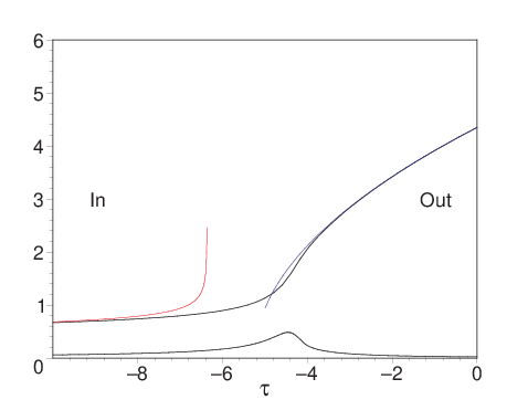
We fix the boundary approximations in and . The the numerical solution gives us for these points
| (20) | |||||
| (21) |
Now with the use of expressions (16) we can fix the approximated solutions. However when we use formula (16) directly to calculate parameters in solution (15) for the outer state we obtain complex . It is due to the expression under square is negative. So to put away complex numbers we redefine the exit solution to the form
| (22) |
where
| (23) | |||||
| (24) |
We show in Fig. 1 how these approximated solutions match with solutions obtained numerically. As we can see these approximated solutions well describe the evolution in the neighbourhood of .
III Gravitational waves
We have already mentioned in section I that gravitational waves can be abundantly produced during the accelerating phase. In this section we want to show in details how it works and calculate properties of produced gravitons. To describe the spectrum of gravitons it is common to use the parameter
| (25) |
where is the energy density of gravitational waves and is present critical energy density. Our goal in this section is to calculate the function for the gravitons produced during the super-inflationary phase.
The gravitational waves are the perturbations of the background spacetime in the form
| (26) |
where . Using constraints we can see that tensor have only two independent components and . These components correspond to two different polarisations of gravitational waves. Inserting the perturbed metric (26) to the Hilbert-Einstein action gives the series , where the second order term have a form
| (27) |
and give us the action for the gravitational waves. The two kinds of polarisations are not coupled and can be treated separately. To normalise the action and simplify the notation it us useful to introduce the variable
| (28) |
what leads to the expression for the action in the form
| (29) |
This action is the same like the action for an inhomogeneous scalar field without the potential. Inverse volume corrections can be therefore introduced in the same way like in the case of the scalar field. As we mentioned in Introduction there are also holonomy corrections to this action. Here we consider however the influence from the better examined inverse volume corrections.
As it was shown by Mulryne and Nunes Mulryne:2006cz, in the context of scalar field perturbations, it is useful to introduce the variable and rewrite the action (29) with quantum corrections to the form
| (30) |
where
| (31) |
Till now the considerations of the gravitational waves has been purely classical. The next step is the quantisation of the classical gravitational waves what brings us the concept of gravitons. To quantise the field we need to firstly calculate conjugated momenta
| (32) |
The procedure of quantisation is the simple change of fields and for the operators just adding hats and to introduce the relations of commutation. We decompose operators considered for the Fourier modes
| (33) | |||||
| (34) |
where the Fourier components fulfil the relations of commutation
| (35) | |||||
| (36) | |||||
| (37) | |||||
| (38) |
To express the Fourier modes in terms of the annihilation and creation operators we need to solve the quantum Hamilton equations
| (39) | |||||
| (40) |
The Hamilton operator have the form
| (41) | |||||
where we inserted decompositions (33) and (34). When we apply the Hamiltonian (41) and the decompositions (33) and (34), the Hamilton equations (39) and (40) take the forms
| (42) | |||||
| (43) |
The general solution of these equations has the form
| (44) | |||||
| (45) |
where . When we insert these solutions to the Fourier decompositions (33) and (34) we simply obtain
| (46) | |||||
| (47) |
The mode functions fulfils the so called Wronskian condition
| (48) |
as a result of relations of commutation (35-38). These relations is important to normalise properly the mode functions.
The Hamilton equations (42) and (43) together with (44) give us the equation for the mode function
| (49) |
This equations has two regimes. The first one called adiabatic corresponds to the situation when . The second one leads to the super-adiabatic amplification and corresponds to the situation when . The creation of the gravitational waves corresponds to the case of the super-adiabatic amplification.
We can now investigate which modes are amplified. The condition corresponds to . In Fig. 2 we see the evolution of . As we see the condition for the creation of gravitational waves is fulfilled in the region of the super-inflation . In the right panel we can see the evolution of for three different values of .
The value of is dimensionless in the undertaken scheme. To obtain a dimensional value we must multiply it simply by the corresponding scale factor which has a dimension of length. The wave number , for example for the final state , corresponds to the frequency
| (50) |
measured today. The important task is to calculate the factor . We can make the decomposition
| (51) |
where
| end of inflation | ||||
| beginning of inflation |
We can assume the sudden reheating approximation and the standard value of e-folding number for inflation . Then increase of the scale factor forms the final state till present value assumes
| (52) |
We had assumed here that , this value can be obtained from numerical simulations like these in Ref. Tsujikawa:2003vr. Now we can return to equation (50) and then calculate the maximal frequency of produced gravitons. From the right panel in Fig. 2 we can see that in the vicinity of we have the transition from positive to negative values of . So as we can see for some we have the transition from the adiabatic to the super-adiabatic regime. From the numerical investigation we obtain . In fact the function , for small values of , is always slightly below zero even for greater values of than . But we assume that this effect is negligible. In fact higher values of easily reach the transplanckian scales and it is not clear that we should trust the standard physics in this regime. The wave number corresponds roughly to the scales . So the value of corresponds to in the final state . Applying equation (50) we obtain the maximal frequency for the present epoch . This value corresponds to the scales . It is instructive to consider the model without inflation. In this situation the maximal frequency of the relic gravitons would be what is extremely huge number. In fact it is possible that GUT energy scale and inflation cover each other in some place. It was somehow one of the motivation to introduce inflation to solve the problem of topological defects. In the case when the GUT scale occurs after thee reheating the problem of topological defects must be solved in a different way. We mention this problem to show that it is possible that the value can be lower than calculated before.
After this analysis we can return now to equation (49). We need to use the definition of the quantum correction and effective mass in the quantum regime. It is also useful to rescale the conformal time and introduce . We will back later to the previous definition because an additional degree of freedom is necessary to fit properly the boundary solutions with numerical one. Equation (49) takes the form
| (53) |
and the general solution in terms of Bessel functions have the form
| (54) |
with
| (55) | |||||
| (56) |
With the use of the Wronskian condition (48) we can rewrite the solution (54) to the form
| (57) |
where we introduced Hankel functions defined as
| (58) | |||||
| (59) |
and the constants and enjoy the relation . To fix values of the constants and we must consider the high energy limit, namely . In this limit the Bessel functions behave as follow
| (60) | |||
| (61) |
what give us and . Classically the limit corresponds to advanced solution called the Bunch-Davies vacuum . Generally the limit obtained here differs from the classical one but can be restored taking . Then to obtain the proper high energy limit we must choose and . Applying evaluated values of and to the solution (57) we finally obtain mode functions for the initial state
| (62) | |||||
| (63) |
where
| (64) |
The functions were calculated from relation showed earlier. We had used also the expression for derivative of the Hankel functions in the form
| (65) |
Similar investigations lead to the expression for the mode functions for the final state. We must remember that it is however not only a simple set but also the change of the solution for the scale factor to this expressed by (22). In this case we obtain
| (66) | |||||
| (67) |
Now we are ready to consider the creation of the gravitons during the transition from some initial to final states. The initial vacuum state is determined by , where is the initial annihilation operator for . The relation between annihilation and creation operators for the initial and final states is given by the Bogoliubov transformation
| (68) | |||||
| (69) |
where . Because we are working in the Heisenberg description the vacuum state does not change during the evolution. It results that is differ from zero when is a nonzero function. This means that in the final state graviton field considered is no more in the vacuum state without particles. The number of produced particles in the final state is given by
| (70) |
Using relations (44)and (45) and the Bogoliubov transformation (68) and (69) we obtain
| (71) | |||||
| (72) |
where simplifications come from the Wronskian condition (48). In the calculations we set and . These boundaries fully cover the region of gravitational waves creation. The energy density of gravitons is given by
| (73) |
where we used definition (70). The expression for the parameter defined by (25) takes now the form
| (74) |
where
| (75) |
In the calculations we set present value of the Hubble factor for . In Fig. 3 we show spectrum calculated with formula (74). The obtained spectrum is extremely weak in the present epoch. The reason of this tiny amount of the background gravitons is the presence of the standard inflationary phase. The super-inflationary phase is placed before the inflation so the energy of gravitons decreases about times during this further phase.
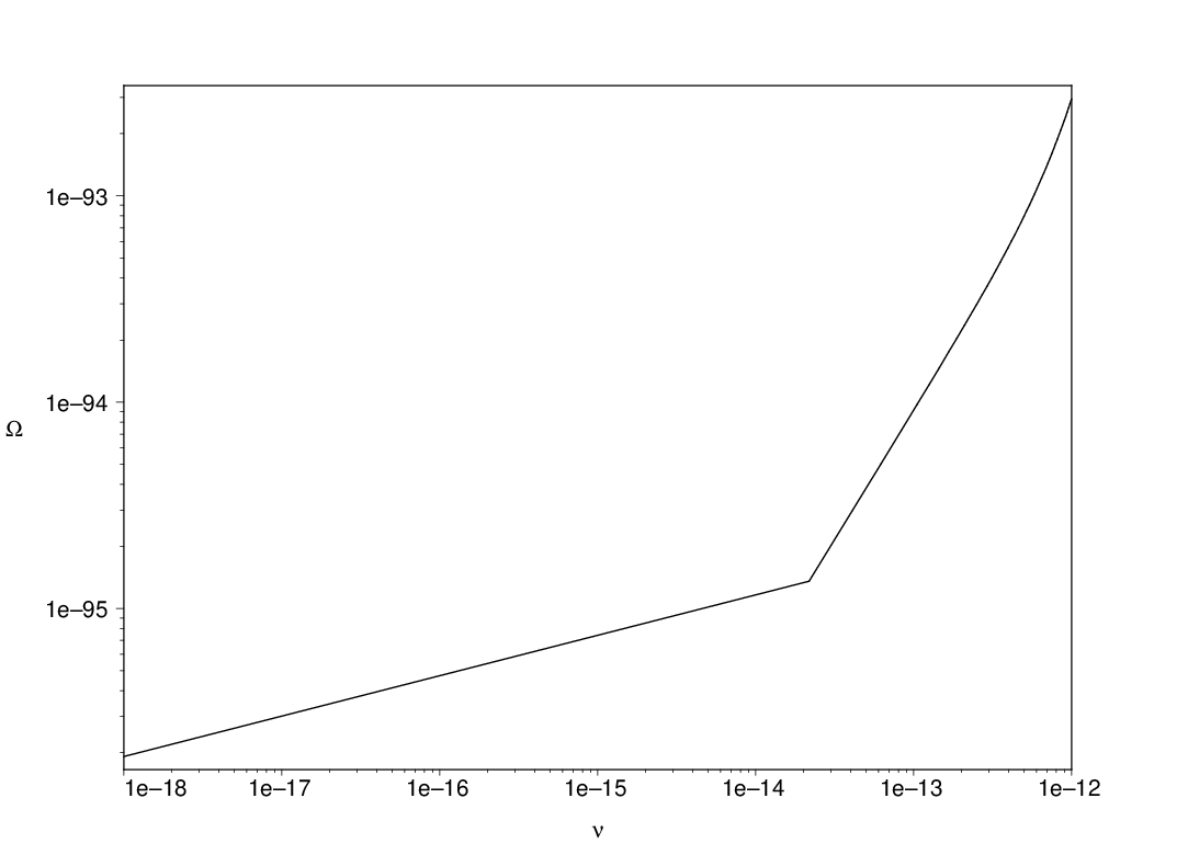
To see better how presence on the inflation affect this spectrum we show in Fig. 3 the spectrum of relic gravitons in the model without the inflationary phase.
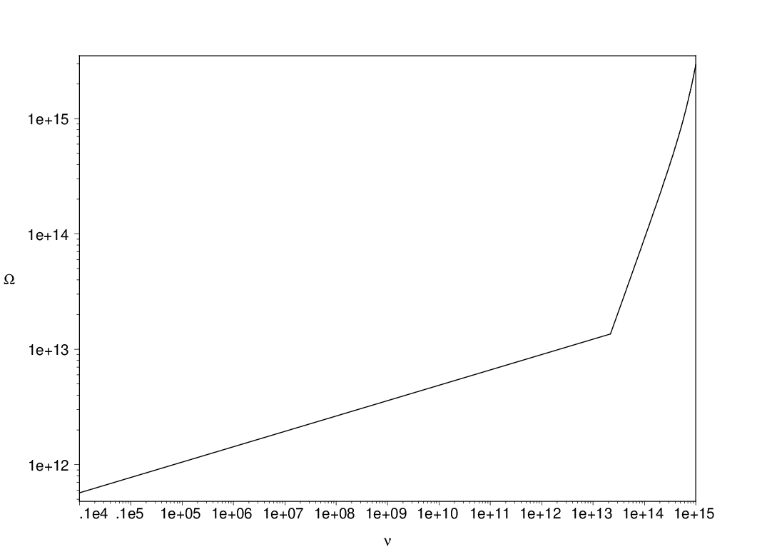
It is clear that in such a model amount of relic gravitons would be extremely large. As we mentioned before it is possible that GUT energy scales cover partially with the inflation. In this situation the present amount of the relic gravitons would be higher than this in Fig. 3 and reaches to higher energies. For the present state we do not know the duration of the inflationary phase exactly. To estimate this value it is necessary to measure the spectrum of both scalar and tensor parts of primordial fluctuations produced during the standard inflation. For the present day we know only the contribution from the scalar part. The further generation of CMB telescopes in needful to improve the knowledge the properties of inflation. From our calculation we can see however that the inflationary phase is necessary. Without the inflation after the super-inflation the present amount of gravitons would be easily in reach of present observational skills. From this point of view we have found the next motivation to support the inflationary model.
IV Summary
In summary, we have calculated the spectrum of gravitons produced during the super-inflationary phase induced by Loop Quantum Gravity effects. In the calculations we considered inverse-volume corrections to the dynamics and to the equation for the tensor modes. We have solved analytically equation for the tensor modes in the quantum and classical regimes. Both solutions we had matched by numerical solution for background dynamics. We have obtained spectra of relic gravitons for the models considered. In the first model we assumed the presence of the inflationary phase after the super-inflation. In that case we obtained presently a negligible amount of relic gravitons. However in the second model without inflation the present amount of graviton background would be unnaturally high. This results state that the period of inflation after the super-inflation is necessary to avoid the problem of relic gravitons. Nowadays the main motivation to introduce the inflationary phase comes from ability to creation of fluctuations. Our investigations based on loop quantum cosmology support the inflationary model.
Results obtained in this work differ from our previous investigations Mielczarek:2007zy. The difference comes mainly from different assumptions about the evolution of the Universe after the super-inflation. The previous results correspond to the situation when inflation and GUT energy scales cover each other rather than to the case of very short inflation. In this paper we have considered both models agreeing with the present paradigm and its modification.
Acknowledgements.
This work was supported in part by the Marie Curie Actions Transfer of Knowledge project COCOS (contract MTKD-CT-2004-517186).References
- (1) L. P. Grishchuk, Sov. Phys. JETP 40 (1975) 409 [Zh. Eksp. Teor. Fiz. 67 (1974) 825].
- (2) B. Abbott et al. [LIGO Scientific Collaboration], Nucl. Instrum. Meth. A 517 (2004) 154 [arXiv:gr-qc/0308043].
- (3) G. Cella, C. N. Colacino, E. Cuoco, A. Di Virgilio, T. Regimbau, E. L. Robinson and J. T. Whelan, Class. Quant. Grav. 24 (2007) S639 [arXiv:0704.2983 [gr-qc]].
- (4) B. Abbott et al. [ALLEGRO Collaboration], arXiv:gr-qc/0703068.
- (5) M. Bojowald, Living Rev. Rel. 8 (2005) 11 [arXiv:gr-qc/0601085].
- (6) M. Bojowald, Phys. Rev. Lett. 89 (2002) 261301 [arXiv:gr-qc/0206054].
- (7) E. J. Copeland, D. J. Mulryne, N. J. Nunes and M. Shaeri, arXiv:0708.1261 [gr-qc].
- (8) J. Mielczarek and M. Szydlowski, arXiv:0705.4449 [gr-qc].
- (9) M. Bojowald and G. M. Hossain, arXiv:0709.2365 [gr-qc].
- (10) A. Ashtekar, Phys. Rev. D 36 (1987) 1587.
- (11) M. Bojowald, Class. Quant. Grav. 19 (2002) 5113 [arXiv:gr-qc/0206053].
- (12) J. E. Lidsey, D. J. Mulryne, N. J. Nunes and R. Tavakol, Phys. Rev. D 70 (2004) 063521 [arXiv:gr-qc/0406042].
- (13) D. J. Mulryne and N. J. Nunes, Phys. Rev. D 74 (2006) 083507 [arXiv:astro-ph/0607037].
- (14) S. Tsujikawa, P. Singh and R. Maartens, Class. Quant. Grav. 21 (2004) 5767 [arXiv:astro-ph/0311015].