The Polyakov Loop and the Eigenvalues of the
Dirac Operator

Lattice simulations suggest that the chiral phase transition and deconfinement phase transition appear at the same temperature. It is believed that there is a connection between both phase transitions. While for the chiral phase transition we have a well established picture of the symmetry breaking mechanism the picture of the deconfinement phase transition remains unclear. Although there has been much progress in the last years the final link connecting both phase transitions is still missing.

The order parameter of the chiral phase transition is the chiral condensate $\langle\bar{q}q\rangle$. Banks and Casher [1] related the chiral condensate to the eigenvalue density $\rho$ of the Dirac operator near zero,

Recently, Gattringer [2] established a formula which relates the eigenvalues of the Dirac operator to the Polyakov loop $P$, the order parameter of the deconfinement phase transition in the quenched approximation. This relation provides a natural link between the chiral condensate and the Polyakov loop via the eigenvalues of the Dirac operator. The hope is to obtain some insight into how both phase transitions are connected.

After a short introduction we will discuss several aspects of this new relation between the Polyakov loop and the eigenvalues, in particular we focus on the volume scaling and the continuum limit. We will present numerical results for both quenched and dynamical QCD and will also compare to the free case.

Starting point of our discussion are the eigenvalues $\lambda$ of the massless staggered Dirac operator, $\hbox to0.0pt{\,/\hss}{{D}}\Psi=\pm\mathrm{i}\lambda\Psi$ with $\lambda real>0$. The massless staggered Dirac operator is defined by

where $\eta_{x\mu}$ is the usual staggered phase factor and $U_{x\mu}$ are the link variables. Note that we use periodic boundary conditions in all four directions for the calculation of the eigenvalues. The Polyakov loop is defined by $P=\frac{1}{N_{c}\,N_{s}^{3}}\sum_{\vec{n}}\mathrm{Tr}_{c}\left[\prod_{n_{4}=1}^{N_{t}}U_{4}(\vec{n},n_{4})\right]$ and can be expressed in terms of the eigenvalues in the following way [2],

$N_{s}$ and $N_{t}$ is the spatial and temporal extension, respectively, and $\mathrm{Z}_{3}=\{1,z,z^{\ast}\}$. Note that $N_{t}$ has to be even for staggered fermions. The sum over $i$ in Eq. 3 is meant to sum over all eigenvalues $\lambda_{i,X}$, where $\lambda_{i,X}$ stands for the eigenvalues calculated on a given gauge configuration which is $\mathrm{Z}_{3}$–rotated by $X\in\mathrm{Z}_{3}$. To be less confusing, for a given gauge configuration we generate all three $\mathrm{Z}_{3}$–rotated gauge configurations and calculate all eigenvalues of the Dirac operator for each of the three configurations. The Polyakov loop can then be expressed as a sum over all eigenvalues calculated on all three rotated gauge configurations, Eq. 3. By looking at Eq. 3 one immediately may ask what part of the eigenvalue spectrum contributes most to the Polyakov loop. To answer this question one introduces the following cumulative sum,

where we sum over all eigenvalues up to a certain (maximal) value $\lambda$. Let us briefly make some comments on this formula before discussing an example. Note that the sector where the Polyakov loop sits for a given configuration (at $T>T_{c}$) is solely determined by multiplying the $\lambda_{i,X}$’s with the appropriate $Z_{3}$–factors. Let us assume for the moment that the gauge configuration corresponding to $\lambda_{i,1}$ has $P$ in the real sector. Remember that the two complex sectors of $P$ are physically equivalent. Therefore, the eigenvalues in the complex sectors of the Polyakov loop are approximately the same, $\lambda_{i,z}\approx\lambda_{i,z^{\ast}}$. Making use of this we obtain for Eq. 3 the following approximate relation, $P(\lambda)\sim\sum_{\lambda_{i,X}<\lambda}(\lambda_{i,real}^{N_{t}}-\lambda_{i,complex}^{N_{t}})$. This relation illustrates the fact that $P(\lambda)$ is built up by the ”response” of the eigenvalues on the different $\mathrm{Z}_{3}$ sectors. As an example we have plotted $P(\lambda)$ for a typical gauge configuration in the complex plane on the left hand side of figure 1. On the right hand side we plotted a sketch of the corresponding eigenvalues calculated in the real and complex sector of the Polyakov loop. We observe that for small eigenvalues the complex sector dominates. By looking at our previously derived relation we see that this results in negative values of $P(\lambda)$ while for large eigenvalues it is the other way round. This shows that the change of the eigenvalues with respect to the different sectors of the Polyakov loop is crucial.

Finally, we perform the ensemble average on the absolute value of $P(\lambda)$,

This is the object we will study for the rest of our discussion. At this point, let us draw the reader’s attention to Refs. [3, 4, 5] were similar investigations has been performed using staggered and Wilson fermions.

In this section we present several numerical results for $\left<\left|P(\lambda)\right|\right>$. We start with results for the quenched case where we have used standard Wilson gauge action. The statistic varies from $\sim 10$ configurations for the largest lattice $8^{4}$ up to $\sim 100$ configurations for the smallest lattice. The eigenvalues were calculated on a single work station using the ARPACK library [6].

Let us first take a look at the plot on the upper left side of figure 2 where $T>T_{c}$ and the Polyakov loop is finite. What we notice right away is that the main contribution to the Polyakov loop comes from the large eigenvalues which is somewhat surprising since the physically relevant part of the spectrum should be the infrared. We will comment on this later on. Another surprising observation is the dip of the curves at $\lambda\approx 1.7-1.8$. Naively, one might expect that the cumulative sum $\left<\left|P(\lambda)\right|\right>$ is a monotonically increasing function. However, by looking at figure 1 this behavior becomes clear. The dip in $\left<\left|P(\lambda)\right|\right>$ (curves in the upper left plot of figure 2) corresponds to the region where $P(\lambda)$ (see figure 1) passes zero, the bump in the curves at $\lambda\approx 1.4$ corresponds to the region where $P(\lambda)$ takes its negative values. This structure seems to be quite interesting and one may ask whether it will survive the infinite volume and the continuum limit.

In figure 2 we illustrate the volume dependence of $\left<\left|P(\lambda)\right|\right>$. On the upper plots we show results for three volumes $4^{3}$, $6^{3}$, $8^{3}$ with $N_{t}=4$ at a temperature slightly above $T_{c}$. The plot on the upper right hand side shows rescaled curves where we have fixed $\left<\left|P(\lambda)\right|\right>=\left<\left|P_{8^{3}\times 4}\right|\right>$ at $\lambda=\lambda_{max}$ for all three volumes. Remember that $P(\lambda_{max})$ is just the ordinary Polyakov loop $P$. Beside the curve corresponding to the smallest volume, which shows small deviations, the curves lie above each other. This observation tells one that for $T>T_{c}$ (for sufficiently large volumes) $\left<\left|P(\lambda)\right|\right>$ has the same volume scaling than the Polyakov loop itself. This in turn means that the structure will survive the infinite volume limit.

For $T<T_{c}$ the situation is similar. On the lower left hand side of figure 2 we plotted $\left<\left|P(\lambda)\right|\right>$ for the same three volumes. The lower right plot shows the corresponding rescaled curves where we again fixed $\left<\left|P(\lambda_{max})\right|\right>=\left<\left|P_{8^{3}\times 4}\right|\right>$. Again, the curves lie above each other showing that $\left<\left|P(\lambda)\right|\right>$ scales like the Polyakov loop also below $T_{c}$. Because below $T_{c}$ the Polyakov loop vanishes in the infinite volume limit we find that also $\left<\left|P(\lambda)\right|\right>$ will vanish in this limit. So in this case the structure does not survive the infinite volume limit. Note that knowing the volume dependence of $\left<\left|P(\lambda)\right|\right>$ will keep the computational costs significantly lower because one do not have to perform expensive computations on large volume lattices.

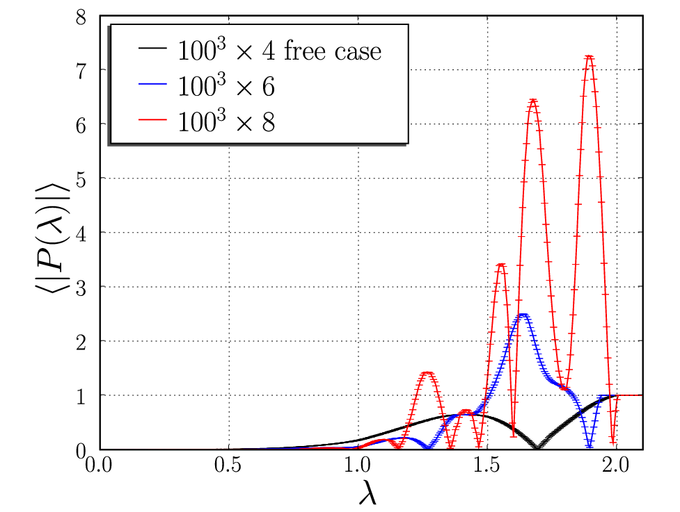
Let us now look at how $\left<\left|P(\lambda)\right|\right>$ behaves as the lattice spacing $a\to 0$. Since for $T<T_{c}$ $\left<\left|P(\lambda)\right|\right>$ vanishes in the infinite volume limit anyway we will discuss only results for $T>T_{c}$. The upper plots in figure 3 illustrate our results for $N_{t}=4,6,8$ at fixed $T\approx 1.2\,T_{c}$ plotted against $\lambda$ in lattice and physical units. Let us focus on the upper left plot. We find that for $N_{t}=6$ there is a bump and a dip in the curve similar to that in the curve for $N_{t}=4$. For $N_{t}=8$ we also observe a large bump but because in this case the statistic is quite limited and the spatial volume is rather small the signal is quite noisy. We notice that, as we go to smaller lattice spacing, the structures in the curves move towards the ultraviolet (UV) part of the eigenvalue spectrum and the Polyakov loop obtains its final value more from the very end of the UV part of the spectrum.

Let us compare these results to the free case where an analytical expression for the eigenvalues is known. The lower plot in figure 3 shows our results in the free case for the same three values of $N_{t}$ at quite large spatial volume. We find that the shape as well as the position of the bumps and dips of the curves are surprisingly similar to the corresponding results of the quenched data (upper left plot). This leads to the following conclusion. As we approach the continuum limit $\left<\left|P(\lambda)\right|\right>$ at small values of $\lambda$ is essentially zero. At somewhat large eigenvalues $\left<\left|P(\lambda)\right|\right>$ starts to show wild fluctuations which cancel out at the very end of the UV part of the eigenvalue spectrum where the Polyakov loop obtains its final value.

We remark that it might be not too surprising that the Polyakov loop is dominated by the UV part of the eigenvalue spectrum as the Polyakov loop is related to the propagation of an infinitely heavy quark. By looking at the quark propagator in the spectral representation,

where $\psi_{\lambda}(x)$ are the normalized eigenvectors of the Dirac operator, we note that the eigenmodes under the sum are weighted by $(\lambda+\mathrm{i}m)^{-1}$. For a very heavy quark (as $m\to\infty$) the relative weight of each eigenmode becomes approximately the same. Therefore, UV eigenmodes can dominate the propagation of an infinitely heavy quark, i.e. the Polyakov loop.

Finally, we compare the quenched results to dynamical results using $p4fat3$ fermions with improved gauge action and quark masses $m_{q}$=0.0065 and $m_{s}$=0.065, see Ref. [7]. On the left (right) hand side of figure 4 we plotted $\left<\left|P(\lambda)\right|\right>$ for $T>T_{c}$ ($T<T_{c}$). Surprisingly, there is no qualitative difference in the behavior of $\left<\left|P(\lambda)\right|\right>$ in the dynamical case.

In this work we have studied the connection between the Polyakov loop and the eigenvalues of the Dirac operator using $\left<\left|P(\lambda)\right|\right>$. We have focused on the volume dependence and the continuum limit. We have found that the dominant contribution to the Polyakov loop comes from the very end of the UV part of the eigenvalue spectrum. We also compared our results to the free case. A comparison between full QCD and quenched QCD seems to show no qualitative difference.

Our findings suggest that the dependence of the eigenvalues on the different $\mathrm{Z}_{3}$ sectors of the Polyakov loop seems to be crucial. Aiming at the connection between confinement and chiral symmetry breaking our findings can be concluded in the following picture. Above $T_{c}$ the eigenvalues $\lambda$ show a strong dependence on the different sectors of the Polyakov loop resulting in wild fluctuations in $\left<\left|P(\lambda)\right|\right>$. These fluctuations cancel out in a way that the Polyakov loop obtains its finite value from the very end of the UV spectrum. At the same time, since the chiral condensate is zero above $T_{c}$, the infrared (IR) part of the spectrum shows a vanishing density of eigenvalues.

Below $T_{c}$ the dependence of the eigenvalues on the Polyakov loop sectors vanishes in the infinite volume limit which leads to a vanishing $\left<\left|P(\lambda)\right|\right>$. In particular $\left<\left|P(\lambda)\right|\right>$ vanishes at the UV leading to a Polyakov loop $\left<\left|P\right|\right>=0$. At the same time, the eigenvalue density at the IR part of the spectrum becomes finite since chiral symmetry is broken.