Global properties of Stochastic Loewner evolution driven by Lévy processes
Abstract
Standard Schramm-Loewner evolution (SLE) is driven by a continuous Brownian motion which then produces a trace, a continuous fractal curve connecting the singular points of the motion. If jumps are added to the driving function, the trace branches. In a recent publication [1] we introduced a generalized SLE driven by a superposition of a Brownian motion and a fractal set of jumps (technically a stable Lévy process). We then discussed the small-scale properties of the resulting Lévy-SLE growth process. Here we discuss the same model, but focus on the global scaling behavior which ensues as time goes to infinity. This limiting behavior is independent of the Brownian forcing and depends upon only a single parameter, , which defines the shape of the stable Lévy distribution. We learn about this behavior by studying a Fokker-Planck equation which gives the probability distribution for endpoints of the trace as a function of time. As in the short-time case previously studied, we observe that the properties of this growth process change qualitatively and singularly at . We show both analytically and numerically that the growth continues indefinitely in the vertical direction for , goes as for , and saturates for . The probability density has two different scales corresponding to directions along and perpendicular to the boundary. In the former case, the characteristic scale is . In the latter case the scale is for , and for . Scaling functions for the probability density are given for various limiting cases.
1 Introduction
The study of random conformally-invariant clusters that appear at critical points in two-dimensional statistical mechanics models has been made rigorous with the invention of the so-called Schramm-Loewner evolution (SLE) [2]. SLE refers to a continuous family of evolving conformal maps that specify the shape of a part of a critical cluster boundary. By now SLE has been justly recognized as a major breakthrough, and there are several review papers and one monograph devoted to this beautiful subject, see Refs. [3, 4, 5, 6, 7, 8, 9, 10]
SLE describes a curve, called trace, growing with time from a boundary in a two-dimensional domain which is usually chosen to be the upper half plane. SLE is based on the Loewner equation in which the shape of the growing curve is determined by a function of time which in SLE is taken to be a scaled Brownian motion. Such a choice of the driving function produces continuous stochastic, fractal and conformally invariant curves, — the kind that appears as the scaling limit of various interfaces in many two-dimensional critical lattice models and growth processes of statistical physics. Well-known examples include boundaries of the Fortuin-Kastelyn clusters in the critical -state Potts model, loops in the model, self-avoiding and loop-erased random walks.
In Ref. [1] we generalized SLE to a broader class for which is a Markov process with discontinuities. More specifically, we have studied the Loewner evolution driven by a linear combination of a scaled Brownian motion and a symmetric stable Lévy process. The growing curve then exhibits branching. This generalized process might be useful to describe many tree-like growth processes, such as branching polymers and various branching growth processes which evolve in time.
Such generalized SLEs driven by Lévy processes (Lévy-SLE for short) have also been of interest to mathematics community. Our results [1] on various phase transitions in Lévy-SLE have been put on rigorous basis in Ref. [11], and further properties have been studied in Refs. [12, 13]. The interest of mathematicians in these Lévy-SLE processes is partially motivated by the suggestion [13, 14] that they may produce fractal objects with large values of multifractal exponents for harmonic measure. Harmonic measure can be thought of as the charge distribution on the boundary of a conducting cluster. On fractal boundaries such a distribution is a multifractal, and in the case of critical clusters (whose boundaries are SLE curves) the full spectrum of multifractal exponents has been obtained analytically, see Refs. [14, 15, 16, 17, 18] for various derivations and discussion.
While our previous paper [1] focused on local properties of Lévy-SLE, here we study the global behavior of the growth in the upper half plain. The present paper is structured as follows. In Section 2 we define our model and briefly state our previous results on phase transitions in the local behavior of the model. We also present our new results on the global behavior of Lévy-SLE. In Section 3 we derive the Fokker-Planck equation governing the evolution of the probability distribution for the tip of the Lévy-SLE. The equation is our main tool for analysis of the long time global behavior of the growth. We give a qualitative description of the growth and explain the approximations that go into the solution of the Fokker-Planck equation in Section 4. Actual solution of the Fokker-Planck equation and comparison with results from numerically calculated trajectories is given in Section 5. We conclude in Section 6. Some technical details are presented in Appendices.
2 The model and the results, old and new
Loewner evolution is a family of conformal maps that appears as the solution of the Loewner differential equation (see, for example, Ref. [3] for details)
| (1) |
valid at any point in the upper half plane until (and if) this point becomes singular at some (possibly infinite) time : . The set of all singularities is called the hull and the point at which the hull grows is called the tip. The tip is defined via its image . More formally,
| (2) |
where the limit is taken in the upper half plane. The trace is the path left behind by the tip (the existence of the trace in the setting of this paper has been shown in Ref. [12]). The shape of the growing trace (and the hull) is completely determined by the driving function . At any time the function conformally maps the exterior of the growing hull to the upper half plane, see Fig. 1. We refer to the plane where the growth occurs as “the physical plane”, and to the plane as “the mathematical plane”.

Naturally, if is a stochastic process the shape of the growing trace is also stochastic. The growth process is then a stochastic (Schramm-) Loewner evolution (SLE). The standard SLE has a driving function , where is a normalized Brownian motion and is the diffusion constant. Many important properties of this process have been established in Ref. [19].
In Ref. [1] we have generalized SLE to
| (3) |
where is a normalized symmetric -stable Lévy process [20, 21, 22, 23], and is the “diffusion constant” associated with it. The process is composed of a succession of jumps of all sizes. Unlike a Brownian motion, is discontinuous on all time-scales. Therefore, the addition of a Lévy processes to the driving force of SLE introduces branching to the trace.
The probability distribution function of is given by the Fourier transform
| (4) |
As it is known in the theory of stable distributions [23], only for this Fourier transform gives a non-negative probability density. For the function decays at large distances as a power law:
| (5) |
so that the process scales as
| (6) |
for any . For this average is infinite. For the process is the standard Brownian motion and is Gaussian.
We studied the short-distance properties of the Lévy-SLE process in Ref. [1]. At short times and distances the process is dominated by the Brownian motion and the deterministic drift term (see Eq. (13)), whereas at long times it is dominated by Lévy flights. The crossover between short and long time behavior happens at the time
| (7) |
This also defines a spatial crossover at length scales . For scales smaller than the trace behaves like standard SLE, while for scales much larger than it spreads in the direction forming tree-like structures.


In our previous paper [1], using both analytic and numerical considerations, we determined the probability that a point on the axis is swallowed by the trace. The trace shows a qualitative change in its small-distance, small-time behavior as and each pass though critical values, respectively at four and one. The transition at is quite analogous to the known transition of standard SLE [19]. For the new transition at , the trace forms isolated trees when or a dense forest when .
The latter phase transition at was recently studied rigorously in Ref. [11] which expanded the implications of the phase transition to the whole plane at the limit . For a point in the upper half plane is swallowed almost surely for , while it is swallowed with probability smaller than one for . For and the swallowed points on the plane form a set of measure zero.
The large-scale implications of the transition can be seen in Figure 2 which shows the shape of the trace at long times. For the stochastic evolution produces isolated tree-like structures which are limited in height. For the evolution produces an “underbrush” in which structures pile on one another and thereby continue to increase their height.
In the rest of the paper we establish the following. The growth at long times is characterized by two very different length scales and (with ) which can be thought of as the typical size of the growing hull in the and directions. More specifically, we find that
| (8) | ||||
| (9) |
(The constants and depend upon .) These scales enter the scaling form of the joint probability distribution for the real and imaginary parts of the tip of the Lévy-SLE, for which we give explicit results in various limiting cases in Section 5, where we also compare analytical results with extensive numerical simulations.
3 Derivation of the Fokker-Planck equation
We are interested in characterizing the probability distribution for the point at the tip of the trace in the ensemble provided by different realizations of the SLE stochastic process. Eq. (2) implies then that we should study the inverse map . However, this is rather difficult, since the map satisfies a partial differential equation instead of an ODE. There is a way out which is rather well known and has been successfully used before [13, 14, 19]. It happens that one needs to consider the backward time evolution:
| (10) |
The relation of the original Loewner evolution (1) and the backward one (10) in the stochastic setting is as follows. If is a symmetric (in time) process with independent identically distributed increments, which is the case for a Lévy process, then it is easy to show that for any fixed time the solution of the backward equation (10) has the same distribution as , see Refs. [13, 19]. Using the symbol for equality of distributions for random variables, we can write
| (11) |
It is useful to introduce a shifted conformal map
| (12) |
for which the Loewner equation acquires the Langevin-like form:
| (13) |
assuming that vanishes at . The first term is a deterministic drift and the second — a random noise. The tip is now mapped to zero, and this can be taken as the definition of the tip. More formally,
| (14) |
where the limit is taken in the upper half plane.
In terms of the shifted map the equality of distributions (11) can be written as
| (15) |
The left hand side of this equation satisfies the Langevin-like equation
| (16) |
and in particular, if we set in this equation, the resulting stochastic dynamics should be the same as that of the tip of the trace .
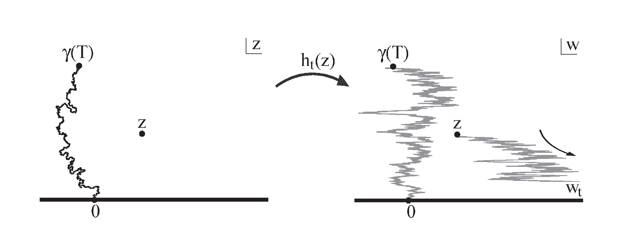
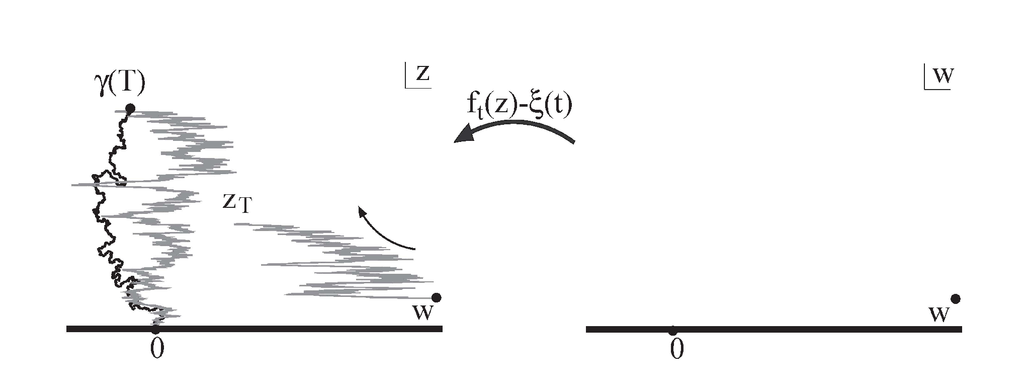
Before we convert the Langevin-like equation (16) to our main analytical tool, the corresponding Fokker-Planck equation, let us review again the correspondence between the forward and backward flows and illustrate it with figures. Equation (13) describes a flow in which follows a trajectory of a particle in the plane, being its initial position. Separating the real and imaginary parts of , we get a system of coupled equations
| (17) |
describing such a trajectory. As in many modern versions of dynamics, all initial conditions and hence all trajectories are considered at the same time, forming an ensemble. Two such trajectories are presented on the top panel in Fig. 3. For a generic initial point the trajectory goes to infinity in the horizontal direction, while the vertical coordinate monotonously decreases. However, if the initial point happens to be a point on the SLE trace, the forward trajectory hits the origin in the mathematical plane exactly at time .
Conversely, we can fix a point in the mathematical plane and follow the motion of its image under the map in the physical plane, with the initial condition . In components , the trajectories of this backward flow satisfy the system of equations
| (18) |
The two trajectories shown on the bottom panel in Fig. 3 precisely retrace the trajectories of the forward flow shown on the top panel. This has been achieved by driving the backward evolution (18) by the time reversed noise as compared to the forward evolution. In this case the final point of the trajectory that started at the origin coincides with the tip of the trace at that time, but the rest of the trajectory does not follow the SLE trace. If we drive the backward flow by an independent copy of , then even the final point will be different from , but in the statistical ensemble and will have the same distribution.
Now we can introduce the probability distribution function of the process in the physical plane defined by:
| (19) |
From Eqs. (3, 18) it follows immediately that satisfies the following (generalized) Fokker-Planck equation:
| (20) |
Here (sometimes also written as ) is the Riesz fractional derivative, which is a singular integral operator whose action is easiest to describe in the Fourier space: if is the Fourier transform of a function , then the Fourier transform of is .
As we have discussed, at long times the growth is dominated by the stable process in the driving function (3), and we can set . So our main analytical tool is the following Fokker-Planck equation:
| (21) |
Let us discuss the boundary and initial conditions for this equation. The initial condition for the Fokker-Planck equation (21) depends on the initial conditions , in the stochastic equations (18). For the distribution of the SLE tip the appropriate initial conditions are , , where is an infinitesimal positive number. For the exact Fokker-Planck equation (20) this translates into the initial condition
| (22) |
However, for the approximate equation (21) the situation is more subtle. The crossover time . For the drift in the direction (towards ) dominates over the Lévy term. For the opposite is true. A simple picture is then that before the initial function is advected by the drift velocity in the direction. By the time it becomes
| (23) |
This is the initial value that we shall assume for our problem. In the following sections we will mostly use the notation , using the explicit expression when necessary.
Let us comment that if we tried to be more careful and included the effects of the Brownian forcing before the crossover time , then the distribution at time would not only be advected to but would also broaden to a Gaussian with variance . This refinement would not change any arguments in the later sections, since all we need there is that the Fourier transform in of the initial distribution is broader than for long times, see the discussion preceding Eq. (36). This is a good approximation for both the initial distribution (23) or its Gaussian variant for sufficiently long times, and becomes better and better as time increases.
As for the boundary conditions at , we have no need to be very explicit about them, since vanishes for , and our equations of motion (18) represent a situation in which continually increases as increases, so that will also vanish for at all times .
4 Qualitative description, distance scales
In this section we analyze in qualitative terms the long-time limit of the evolution of the tip , by looking at the consequences of equations (18). According to the discussion in the previous section, and have the same joint distribution as and .

For small times, up to the crossover time , the drift term in the Langevin equation dominates over the Lévy noise. Therefore, both and , and as well, grow as . For larger times, , there are two different characteristic length scales, and . In this regime the forcing is dominated by the Lévy process . The probability for a total motion over a time for this process is described by Eq. (4). Typically the motion is dominated by a single long jump, and the jump has an order of magnitude
| (24) |
(This can be understood as rescaled fractional moments , see Eq. (6)) Since the typical jumps of become arbitrarily large at long times, also becomes large, and therefore, the drift term in the first equation of (18) becomes negligible. In this limit, behaves like the driving force, and we find
| (25) |
The Loewner evolution with Levy flights produces, in general, a forest of (sparse or dense) branching trees, growing form the real axis. The above relation then tells us how the forest spreads along the real axis with time. This distance is marked out on the plots of trees shown in Figure 2.
Numerical implementation of the Langevin equation (16), details of which are presented in Appendix A.1, confirms these qualitative arguments. Figure 4 compares the estimate of Eq. (25) with numerical calculations of the trace via simulations of Eq. (16). The agreement is excellent.
Next we turn to a typical distance in the coordinate. Figure 2 clearly shows that this characteristic distance is much smaller than . We understand this as follows. If were zero, the second equation in (18) would give . Clearly, any non-zero only slows down the growth of . We then conclude that , and therefore the height of the trees produced by the SLE process cannot grow with time faster than . Since , it means that always grows slower than and they become widely separated at long times. Our major result is that the growing trees spread faster horizontally than they grow vertically. Hence, we have
| (26) |
An estimate of the scaling of can be obtained from the second equation in (18) where we replace by the Lévy process and average over it using the probability distribution (4). This gives a typical behavior of :
| (27) |
To estimate the integral we can drop the term in the exponent, since this quantity is of order . Thus we get
| (28) |
The time integration then gives a result that the length scale for the direction is
| (29) |
Here is formally the constant of integration, but it should really be thought of as an adjustable constant inserted to make up for any errors we might have made in doing the integrals. In particular, it takes care of any effects from the early-time region, where we surely do not have the calculation under control.

The phase transition at is manifested by a qualitative difference between and . From (29) we can see that while for the average height of the trees grows to infinity as , while for it saturates at a finite value . Figure 5 provides an illustration of the phase transition at separating different behaviors. More detailed comparison between our analytical predictions and numerical simulations is provided in the next Section.
5 Solving the FPE
In order to quantify these predictions we need to return our attention to the Fokker-Plank equation (21). If we perform the Fourier transform in and integrate in time we can find a compact form of this equation, which reads
| (30) |
where is the Fourier transform of the initial distribution (23). At long times is spread over the scale as a function of . Its Fourier transform , as a function of , is significantly non-zero on the scale . At the same time, due to the exponential factors , the relevant values of in the integrals in Eq. (30) are of the order . The scale is much larger than the range where is non-zero, hence, when integrating over we can use the approximation
| (31) |
The Fokker-Planck equation then reads:
| (32) |
This is the main approximation that we will use in order to study the behavior of the Lévy-SLE process at large times.
Notice here that the distribution function , for every and , depends only on the initial condition and the history of the distribution at for earlier times . Therefore, in order to study the probability density function described by the Fokker-Planck equation, we first need to calculate the behavior of this distribution for small , that is . Then, by substituting in Eq. (32), we can in principle estimate the full distribution. However, in this paper we are mostly interested in the way this process grows in the direction. Hence, we will first find which characterizes the growth near , and then obtain the distribution
| (33) |
of ’s integrated over all by setting in (32):
| (34) |
This equation immediately leads to the average , which is understood as the average over all :
| (35) |
Therefore, the distribution and its mean in Eqs. (34) and (35) depend only on the behavior at at times . This is a direct implication of Eq. (32) and our main approximation (31).
Let us emphasize again that our approximation works in the long time limit. We will assume that we can use approximate expressions in time integrals for all . Thus, we will treat all time integrals as . The corrections come from short times, and we cannot extract them from our analysis. They all will be hidden in the terms dependent on the lower limit of the time integrals. In several cases the lower cut-off at is necessary to avoid spurious divergencies.
Let us now consider . A closed equation for this quantity results from integrating Eq. (32) over . To do this we observe that in the first term (the initial value at ) for the relevant values of the function is much broader in than at long times. Hence, in the integral over we can replace by its value at . Then it follows that
| (36) |
where the scale is defined as
| (37) |
and
| (38) |
Equation (36) is easily solved after performing the Laplace transformation in time . For the transform
| (39) |
we obtain an ordinary differential equation
| (40) |
where
| (41) |
and . Using the initial condition , the straightforward solution of Eq. (40) is
| (42) |
The inverse Laplace transform of this solution gives .
Notice that (42) is valid only for . Since our approximations only work at long times, we expect our solution to give good results for . The approximations will usually result in the necessity to introduce a fitting parameter (called “correction” in the discussion after Eq. (35)) in the time evolution of averages for the process. Moreover, there is an upper cut-off that stems from the Langevin equation and the fact that cannot grow faster than (see previous section). Since we used this fact while making the approximations that lead to Eq. (32), the range of validity of our solution is .
In the following we will analyze the properties of the distributions and in three separate cases , and . For each case we will repeat the following steps: first we calculate from Eq. (42), then, by substituting this solution into Eq. (34), we will calculate the average height and the distribution . In these calculations we need approximate expressions for the function . These expressions are derived in Appendix A.2.
5.1 Results for
In this case we can use the approximation (86) from Appendix A.2 for and . Eq. (42) then gives
| (43) |
To calculate the time dependence of the distribution we take the inverse Laplace transform:
| (44) |
As usual, the integration contour in the last equation goes along a vertical line Re, where should be greater than the real part of any singularity of the integrand. Changing the integration variable to we obtain that answer which, apart from the overall prefactor , has acquired the form of a scaling function:
| (45) | ||||
| (46) |
Since the scaling function depends only on the combination , its derivatives with respect to and are related:
| (47) |
The integrand in Eq. (46) contains a branch cut which we choose to run along the negative real axis. The integration contour can be deformed to go from to along the lower side of the cut, and then from 0 to along the upper side. This leads to the final answer for the scaling function :
| (48) |
The overall prefactor in can be understood as follows. The distribution at long times spreads in the direction up to scale , and in the direction up to scale . The total area “covered” by the distribution scales with time as . Therefore, at the particular value the density decays with time as . However, if we are looking at the distribution of the coordinate for , and its moments , we should divide by the normalization
| (49) |
The normalized distribution is then
| (50) |

Moreover, the integrated distribution exhibits the same scaling as . Indeed, using the relation (47) in Eq. (34) we obtain:
| (51) |
Fig. 6 shows the scaling collapse of the numerically calculated distributions for and three different times. We see that, indeed, is a scaling function of in agreement with our predictions.

We can calculate the asymptotics of the function . For small values of we can neglect the term with in the exponential in Eq. (46), as well as replace the sine function under the integral by its (small) argument:
| (52) |
For large we need to use the steepest descent method for the contour integral in Eq. (46), which results in
| (53) |
We have to remember that we can only trust this result for .
Figure 7 shows a comparison between the numerical data and the theoretical prediction of Eq. (51) for the distribution . While the overall dependence on is similar between the two, we would obtain a better fit for if we redistributed the weight outside this region to the range were Eq. (51) is valid.

Next, we will calculate the time evolution of the average height of the growing trees from Eqs. (35, 49):
| (54) |
Here, all short time contributions are included in . This nicely fits the numerics, see Fig. 8, and reproduces the result (29) of the simple argument using the Langevin equation.

We also want to compare the distribution at to the distribution averaged over all . We calculate the average value (the superscript indicates that this average is calculated at ) from the distribution (50):
| (55) |
The ratio of the two averages (neglecting ) is
| (56) |
This tends to 2 as from above, and to as from below. We observe similar behavior in our numerical results, where the average of at is higher than the overall average (Fig. 9). However, the ratio (56) is not matched exactly. Presumably, this is because we do not have enough data close to and we cannot reach long enough times in order for the various constants (like ) to be negligible, so that Eq. (56) is accurate.
5.2 Results for
Now we use the approximations (79, 84) from Appendix A.2 in Eq. (42). The resulting expression for is difficult to analyze without further approximations. We will evaluate it as well as its inverse Laplace transform with logarithmic accuracy, which amounts to three assumptions. First, we assume that all the logarithms that appear are large compared to constants of order one such as , , etc, which will be neglected. Secondly, the logarithms are assumed to be small compared to power laws for large arguments: . Finally, the logarithms are slow functions as compared to power laws and exponentials, and in integrals can be replaced by their values at the typical scale of variation of the fastest function under the integral. All subsequent equations in this section will be obtained with logarithmic accuracy using these assumptions.
First we have
| (57) |
The time dependence now follows from the inverse Laplace transform, using the same contour integral described in the previous section:
| (58) |
The integral of this expression over
| (59) |
leads to a normalized distribution at :
| (60) |

The mean value of the height of trees near follows from using the same arguments as before:
| (61) |
The average height (over all ) is also found easily from Eq. (35):
| (62) |
As shown in Fig. 10 this is in good agreement with the numerics. The ratio of the two averages in the long time limit is , consistent with the limit of Eq. (56).
The asymptotics of the distribution for small and large values of can be found similar to the case :
| (63) |
Finally, using Eq. (34), we get an expression for the integrated distribution:
| (64) |
The asymptotics of these expression follow as before:
| (65) |
5.3 Results for

In this case we use the approximation (87) from Appendix A.2 leading to
| (66) | ||||
| (67) |
The inverse Laplace transform of this expression gives the leading approximation
| (68) |
The obtained result depends on time only through the overall factor . We can understand this as follows. The distribution at long times spreads in the direction up to the scale but becomes stationary in the direction. Therefore, at the particular value the density decays with time as . However, if we are looking at the distribution of the coordinate for , we should normalize Eq. (68) which gives the truly stationary distribution (normalized by the appropriate choice of )
| (69) |
in agreement with numerics, see Fig. 11, where we actually observe that the integrated distribution coincides with at long times.


The stationary distribution (69) allows us to calculate the average saturated height of the trees:
| (70) |
This is in very good agreement with the numerically calculated values shown in Fig. 12.

Let us discuss now the integrated distribution and its mean . Unfortunately, in the present case (), the Eqs. (34) and (35) do not give reliable results simply because the apparent distribution and saturation height are very sensitive to the lower limit , and the results are of the same order as the initial conditions at . Analytically, we can see that the distribution becomes stationary as , even though we cannot determine . The time independence of the distribution at long times is checked numerically in Fig. 13. Numerics presented in Fig. 11 indicate that (see Eq. (69)) for the appropriate range , and we will discuss why this is true below.

We can also see that the way the average tree height approaches its limiting value is given by the power law
| (71) |
We have previously calculated in Eq. (29) using the Langevin formulation of the process. This result agrees well with numerics, as demonstrated in Fig. 14.

We can argue that and that , if we return to the initial description of the process seen as SLE trees growing forward in time [1]. For the jumps of the Lévy process are large and we know that any new tree is most likely to grow starting from the real axis. The trees are sparse and the new tree will grow isolated from its neighbors, hence it will be identical to any other tree, including the trees that grow close to the origin at . Therefore, we expect the distribution of ’s at to be identical to the distribution at any other . Numerics also support this argument. In Fig. 15 we observe that the average height of the trees is practically independent of the value of . Also, in Fig. 11 we compare and while in Fig. 12 we show that .
6 Conclusions
In this paper we have analyzed the global properties of growth in the complex plain described by a generalized stochastic Loewner evolution driven by a symmetric stable Lévy process , introduced in our previous paper [1]. The phase transition at whose implications for local properties of growth were the subject of Ref. [1], also manifests itself on the whole plane resulting in a rich scaling behavior.
We have used a Fokker-Planck equation to study the joint distribution for the real and imaginary parts of the tip of the growing trace. The presence of the Lévy flights in the driving force imposes very different dynamics in the and directions. While in the direction the process spreads similarly to the Lévy forcing , the SLE dictates , for all values of . This separation of the horizontal and vertical scales in the process allows us to make sensible approximations and explore geometric properties of the stochastic growth in all phases, , , and , both qualitatively and quantitatively.
For , the vertical growth saturates at a finite height . In terms of the picture presented in [1], long jumps occur often so that new trees grow isolated and there is a small chance that the trace grows on an already existing tree.
For , the average height of the process grows as a power law with time. New trees grow close to old ones, so that when the process returns to a previously visited part of the real axis it will have to grow on top of already existing trees. Eventually the trace will grow past any point on the plane.
At the boundary between the two phases, , the height of the process grows logarithmically with time.
7 Acknowledgements
This research was supported in part by NSF MRSEC Program under DMR-0213745. IG was also supported by an award from Research Corporation and the NSF Career Award under DMR-0448820. We wish to acknowledge many helpful discussions with Paul Wiegmann, Eldad Bettelheim, and Seung Yeop Lee. IG also acknowledges useful communications with Steffen Rohde.
Appendix A Appendices
A.1 Numerical calculations
The interpretation of equation (16) is very helpful to our calculations. and the tip of the trace have the same distribution. This allows, instead of calculating the trace for every time and noise realization (), to efficiently collect statistics for the position of the tip by integrating the Langevin equation (16) ().
Following Ref. [1] we approximate by a piecewise constant function with jumps appropriately distributed: for . For such a driving function the process in Eq. (16) can then be calculated numerically as an iteration process of infinitesimal maps [24] starting from the condition as follows:
| (72) |
The infinitesimal conformal map at each time interval is defined by:
| (73) |
The value of is randomly drawn from the appropriate distribution. The number of steps necessary to produce an SLE trace up to step grows only as . All numerical results in the next section have been calculated using the average of Eq. (73) over many noise realizations.
The trace can also be produced directly [1], as , in which case we approximate
| (74) |
However, the number of steps in this method grows as . We used this method to verify that numerically calculated and have identical distributions. Eq. (74) was also used to calculate the traces shown in Fig. 2.
Here, we will assume for simplicity, that is, the driving force is pure Lévy flights . The addition of a Brownian motion will not affect our conclusions. For all realizations of the Lévy-SLE process we take and unless otherwise noted.
A.2 Asymptotics for
Let us consider (we need to use the lower cut off here to have a convergent result for )
| (75) |
where is the incomplete gamma function, and is the exponential integral. Since has the dimension and the meaning of frequency, and we are interested in , we will only need the small argument asymptotics of these functions:
| (76) |
This gives for
| (77) | |||||
| (78) | |||||
| (79) |
For we can set and obtain
| (80) |
and for we can set :
| (81) |
We now turn to the Laplace transform :
| (82) |
Since in the Laplace transform the important values of are the inverse typical time scales, this means that the relevant asympotics of are those with . The opposite case of corresponds to short times, where our basic approximation is invalid. So from now on we will focus on the limit .
This integral can be evaluated exactly in a number of cases. First, when , the integral converges for and gives the same expression as in Eq. (80). Secondly, for the integral converges (for ) for and gives then
| (83) |
All the constants , , and defined above diverge as as . Finally, for we get
| (84) |
In general for , a good approximation for is the sum of expressions in Eqs. (80, 83):
| (85) |
Not only this approximation reproduces the correct limits in Eqs. (80) and (83), but in the limit it also reduces to Eq. (84). This approximation can be obtained by splitting the interval in the integral in Eq. (82) into two at the value and in each resulting integral replace the denominator by the largest term in it.
References
- [1] I. Rushkin, P. Oikonomou, L.P. Kadanoff and I.A. Gruzberg, J. Stat. Mech. P01001 (2006); arXiv: cond-mat/0509187
- [2] O. Schramm, Israel J. Math. 118, 221 (2000); arXiv: math.PR/9904022.
- [3] G. F. Lawler. Conformally invariant processes in the plane. Mathematical Surveys and Monographs, 114. Providence, R.I.: American Mathematical Society, 2005.
- [4] W. Werner, Random planar curves and Schramm-Loewner evolutions, in Lecture Notes in Mathematics, 1840. Berlin, New York: Springer-Verlag, 2004; arXiv: math.PR/0303354.
- [5] O. Schramm, Conformally invariant scaling limits: an overview and a collection of problems, in International Congress of Mathematicians. Vol. I, 513, Eur. Math. Soc., Zürich, 2007; arXiv: math.PR/0602151.
- [6] M. Bauer and D. Bernard, Phys. Rep. 432, 115 (2006); arXiv: math-ph/0602049.
- [7] J. Cardy, Ann. Phys. 318, 81 (2005); arXiv: cond-mat/0503313.
- [8] I. A. Gruzberg, J. Phys. A: Math. Gen. 39, 12601 (2006); arXiv: math-ph/0607046.
- [9] I. A. Gruzberg and L. P. Kadanoff, J. Stat. Phys. 114, 1183 (2004); arXiv: cond-mat/0309292.
- [10] W. Kager and B. Nienhuis, J. Stat. Phys. 115, 1149 (2004); arXiv: math-ph/0312056.
- [11] Q. Guan and M. Winkel, arXiv: math.PR/0606685.
- [12] Q. Guan, arXiv: 0705.2321 [math.PR].
- [13] Z.-Q. Chen and S. Rohde, arXiv:0708.1805v2 [math.PR].
- [14] D. Beliaev and S. Smirnov, Harmonic measure and SLE, arXiv: 0801.1792v1 [math.CV].
- [15] B. Duplantier, Phys. Rev. Lett. 84, 1363 (2000); arXiv: cond-mat/9908314.
- [16] B. Duplantier, in Fractal geometry and applications: a jubilee of Benoît Mandelbrot, Part 2, 365, Proc. Sympos. Pure Math., 72, Part 2, Providence, R.I.: American Mathematical Society, 2004; arXiv: math-ph/0303034.
- [17] E. Bettelheim, I. Rushkin, I. A. Gruzberg, P. Wiegmann, Phys. Rev. Lett. 95, 170602 (2005); arXiv: hep-th/0507115.
- [18] I. Rushkin, E. Bettelheim, I. A. Gruzberg, and P. Wiegmann, J. Phys. A: Math. Theor. 40, 2165 (2007); arxiv: cond-mat/0610550.
- [19] S. Rohde and O. Schramm, Ann. of Math. (2), 161(2), 883 (2005); arXiv: math.PR/0106036.
- [20] D. Appelbaum. Lévy processes and stochastic calculus, Cambridge, U.K.; New York: Cambridge University Press, 2004.
- [21] R. Metzler and J. Klafter, Phys. Reports 339, 1 (2000).
- [22] G. Samorodnitsky and M. S. Taqqu. Stable non-Gaussian random processes: stochastic models with infinite variance, New York: Chapman & Hall, 1994.
- [23] K. Sato. Lévy processes and infinitely divisible distributions, Cambridge, U.K.; New York: Cambridge University Press, 1999.
- [24] M. B. Hastings, Phys. Rev. Lett. 88, 055506 (2002); arXiv: cond-mat/9607021.