1Introduction

arXiv:0710.2640

Time-dependent AdS/CFT Duality II :
Holographic Reconstruction of Bulk Metric
and Possible Resolution of Singularity

Chong-Sun Chu¹, Pei-Ming Ho²

¹

Centre for Particle Theory and Department of Mathematics, Durham University,
Durham, DH1 3LE, UK.
²

Department of Physics and Center for Theoretical Sciences, National Taiwan University, Taipei 10617, Taiwan, R.O.C.

chong-sun.chu@durham.ac.uk, pmho@phys.ntu.edu.tw

Abstract

We continue the studies of our earlier proposal for an AdS/CFT correspondence for time-dependent supergravity backgrounds. We note that by performing a suitable change of variables, the dual super Yang-Mills theory lives on a flat base space, and the time-dependence of the supergravity background is entirely encoded in the time-dependent couplings (gauge and axionic) and their supersymmetric completion. This form of the SYM allows a detailed perturbative analysis to be performed. In particular the one-loop Wilsonian effective action of the boundary SYM theory is computed. By using the holographic UV/IR relation, we propose a way to extract the bulk metric from the Wilsonian effective action; and we find that the bulk metric of our supergravity solutions can be reproduced precisely. While the bulk geometry can have various singularities such as geodesic incompleteness, gauge theory quantum effects can introduce higher derivative corrections in the effective action which can serve as a way to resolve the singularities.

1 Introduction

The understanding of the nature of spacetime singularity, and whether and how it is resolved, is one of the most important question for a quantum theory of gravity. Recently, powerful nonperturbative formulations of string theory such as Matrix theory [1, 2] and AdS/CFT correspondence [3, 4, 5, 6] have been put forward and intensively studied for various applications. While much work has been devoted to the studies of blackhole singularities [7], there were much fewer studies on spacetime singularities of cosmological type. It is desirable to apply these ideas to the studies of time-dependent backgrounds, and try to use them to learn about spacetime singularity. See [8] for recent reviews on approaches to understanding spacelike or null singularities in string theory.

In [9], we constructed a supersymmetric AdS/CFT correspondence for a class of time-dependent II B backgrounds. The supergravity (SUGRA) backgrounds have nontrivial time dependence through a null coordinate. Similar SUGRA backgrounds were also constructed in [10, 11]. In addition we have also constructed the dual gauge theory explicitly [9]. The gauge theory features a time-dependent gauge coupling and a time-dependent axion coupling. The proposed gauge/gravity duality thus constitutes a natural starting point for understanding time-dependent superstring backgrounds from the super Yang-Mills (SYM) theory. Our work was motivated by the earlier works of [12] which proposed to use AdS/CFT correspondence to study a big crunch cosmology; and [13] which proposed to use matrix string theory to study null singularities. For a different approach of applying AdS/CFT to time-dependent backgrounds see [14]. See also [15] for related works.

In our construction [9], the SUGRA metric admits cosmological, null-like singularities for some class of dilaton and axion field configurations. Moreover, since these singularities are situated at a constant $x^{+}$ (rather than localized at finite radial coordinate), their presence can in principle be detected by quantities computed in the dual field theory. In [9], we have carried out a generic analysis at the free field level. We found that the field theory two-point functions computed from the gravity side using the duality is different from the one computed directly from the field theory, which up to a rescaling of fields, is the same as the one defined for an ordinary Minkowskian spacetime. In particular, the SUGRA result is sensitive to the singularity of the spacetime, while the gauge theory result does not see the singularity. That the results differ is not surprising since the SUGRA result is valid in the regime where the t’Hooft coupling is large, while the field theory result is valid when the t’Hooft coupling is small. We interpreted our results as suggesting that the spacetime singularity seen at the SUGRA level could be resolved by $\alpha^{\prime}$ effects of string theory. Similar analysis has also been performed in [16] with the same conclusion.

While this might look encouraging, the following remarks prompt immediately for more detailed studies in the dynamics of the gauge theory. First, the regularity of the field theory 2-point function is demonstrated only at the free field level. When interaction is included, we expect the answer to depend on the coupling, as well as its higher time derivatives. It is therefore possible that the field theory result could reproduce the SUGRA singularity once quantum corrections are included. Secondly, in our work [9], we pointed out that the Einstein equation (see (2) below), which constitutes a constraint on the dilaton and axion field, can be obtained from the requirement of finiteness of the energy momentum tensor in gauge theory. However, this argument is not completely satisfactory as it is based on the validity of the duality. In [9], we conjectured that the Einstein equation could be derived from the the gauge theory at the quantum level. Achieving this would help us to understand better how quantum properties of SYM is mapped holographically to the geometrical properties of spacetime.

The purpose of this paper is to go beyond the free field level analysis and to try to understand the role of the SYM quantum effects in the duality. In particular we propose to identify bulk metric properties from the Wilsonian effective action obtained by intergrating out the high momentum modes.

In section 2 we review our proposal of the time-dependent AdS/CFT duality. In section 3, we demonstrate that by a change of variables, both the SUGRA metric and the SYM Lagrangian can be written in a simpler form. We restate our duality proposal in this frame. In section 4, we present the Feynman rules for our time-dependent SYM theory. The presence of the time-dependent gauge couplings and time-dependent theta angle modify the interaction vertices. In section 5, we compute the 1-loop Wilsonian fermion kinetic term and find that at the leading order of derivative expansion, it allows one to reconstruct the bulk metric of the gravity side. It is straightforward to include the higher order derivative corrections to the holographically constructed bulk geometry and we discuss how spacetime singularity could be resolved.

2 Time-dependent AdS/CFT correspondence: review

In [9], a time-dependent deformation to the original AdS/CFT correspondence was constructed. The non-vanishing fields consist of the Einstein metric

ds^{2}=\frac{R^{2}}{u^{2}}\left(-k^{2}(x^{+})dx^{+}dx^{-}+M_{i}^{2}(x^{+})(dx^{i})^{2}+du^{2}\right)+R^{2}d\Omega_{5}^{2}\qquad(i=2,3),

(1)

an undeformed 5-form, and dilaton and axion fields $\phi(x^{+}),\chi(x^{+})$ . All equations of motion are satisfied provided

\frac{1}{2}(\phi^{\prime})^{2}+\frac{1}{2}e^{2\phi}(\chi^{\prime})^{2}=-\sum_{i=2,3}\left(\frac{M_{i}^{\prime\prime}}{M_{i}}-\frac{2k^{\prime}M_{i}^{\prime}}{kM_{i}}\right),

(2)

which comes from the $(++)$ -component of the Einstein equation.

The SUGRA solution preserves eight II B supersymmetries. Viewed as a deformation of the standard $AdS_{5}\times S^{5}$ , half of the Poincare supersymmetry is preserved, and the conformal supersymmetry is broken. The solution can be obtained from a near horizon limit of a strack of D3 branes with a pp-wave on it. This gives rise to the relation between the radius $R$ and the dilaton [9]

R^{4}=16\pi N\langle g_{s}^{-1}\rangle^{-1}l_{s}^{4},

(3)

where $\langle g_{s}^{-1}\rangle:=\int dx^{+}k^{2}e^{-\phi}/\int dx^{+}k^{2}$ is the $x^{+}$ -average of the inverse of the string coupling $g_{s}=e^{\phi}$ . This relation generalizes the celebrated relation in the original AdS/CFT correspondence, and is a consequence of the BPS property of the stack of pp-wave D3-branes. It is interesting to note that if $\langle g_{s}^{-1}\rangle$ diverges, which could happen if $g_{s}$ goes to zero somewhere, $N$ needs to be infinity even for finite radius $R$ .

We also noted that the supergravity solution is invariant under the scaling transformation

u\to\lambda u,\quad x^{+}\to x^{+},\quad x^{-}\to\lambda^{2}x^{-},\quad x^{i}\to\lambda x^{i}.

(4)

The same symmetry is respected by our time-dependent SYM [9].

The above metric was written down in the Rosen form. One can also perform a change of coordinate [9] to put the metric in the following Brinkman form

ds^{2}=\frac{R^{2}}{u^{2}}\left(-k^{2}(x^{+})dx^{+}dx^{-}+h(x^{+},x^{i})(dx^{+})^{2}+(dx^{i})^{2}+du^{2}\right),

(5)

where

h(x^{+},x^{i})=\sum_{i=2,3}h_{i}(x^{+})\;(x^{i})^{2},\quad\mbox{and}\quad h_{i}(x^{+})=\frac{M^{\prime\prime}_{i}}{M_{i}}-\frac{2k^{\prime}M_{i}^{\prime}}{kM_{i}}.

(6)

Without loss of generality, one can choose the coordinate $x^{+}$ such that $k(x^{+})=1$ . It is then easy to see that this metric has an interesting property, that is, it deviates from the undeformed $AdS$ metric only by the $g_{++}$ (or equivalently the $g^{--}$ ) component, and as a result only the $R_{++}$ component of the curvature tensor is modified. It follows that all the invariants obtained by contracting indices of curvature tensors are exactly the same as pure $AdS$ space. Therefore we believe that this metric is free from stringy ( $\alpha^{\prime}$ ) corrections for the same reason why $AdS$ is an exact consistent background. On the other hand, our background is expected to receive $g_{s}$ corrections due to string loop diagrams.

Provided that the radius $R$ defined by (3) is well defined, we proposed in [9] that the quantum gravity for the time-dependent background (5) is dual to a SYM theory living on the boundary metric

ds_{\mbox{\tiny YM}}^{2}=-k^{2}(x^{+})dx^{+}dx^{-}+h(x^{+},x^{i})(dx^{+})^{2}+(dx^{i})^{2}

(7)

and has a time-dependent Yang-Mills coupling and theta angle

\frac{\theta}{2\pi}+\frac{4\pi i}{g_{{\mbox{\tiny YM}}}^{2}}=\chi+ie^{-\phi}.

(8)

The Lagrangian density is ¹¹ 1 There was a typo in the fermionic part of the axion action $S_{\chi}$ in our previous paper [9]. $\chi$ should be replaced by $\chi^{\prime}$ as in (12). ${\cal L}={\cal L}_{\mbox{\tiny YM}}+{\cal L}_{X}+{\cal L}_{\Psi}+{\cal L}_{\chi}$ , where [9]

	$\displaystyle{\cal L}_{{\mbox{\tiny YM}}}=\frac{\sqrt{-g}}{g_{{\mbox{\tiny YM}}}^{2}}{\rm Tr}\left(-\frac{1}{4}g^{\mu\mu^{\prime}}g^{\nu\nu^{\prime}}F_{\mu\nu}F_{\mu^{\prime}\nu^{\prime}}\right),$		(9)
	$\displaystyle{\cal L}_{X}=\frac{\sqrt{-g}}{g_{{\mbox{\tiny YM}}}^{2}}{\rm Tr}\left(-\frac{1}{2}g^{\mu\nu}D_{\mu}X^{a}D_{\nu}X^{a}+\frac{1}{4}[X^{a},X^{b}]^{2}\right),$		(10)
	$\displaystyle{\cal L}_{\Psi}=\frac{\sqrt{-g}}{g_{{\mbox{\tiny YM}}}^{2}}{\rm Tr}\left(\frac{1}{2}\bar{\Psi}\gamma^{\mu}[-iD_{\mu},\Psi]+\frac{1}{2}\bar{\Psi}\gamma^{a}[X_{a},\Psi]\right),$		(11)
	$\displaystyle{\cal L}_{\chi}=\frac{1}{8\pi^{2}}\mbox{Tr}\left(-\frac{1}{4}\theta(x^{+})\epsilon^{\mu\nu\rho\sigma}F_{\mu\nu}F_{\rho\sigma}+\frac{i}{4}\theta^{\prime}(x^{+})\bar{\Psi}\Gamma^{2}\Gamma^{3}\Gamma^{+}\Psi\right).$		(12)

Here $\Psi$ is a Majorana spinor, $D_{\mu}=\partial_{\mu}+iA_{\mu}$ and $F_{\mu\nu}=\partial_{\mu}A_{\nu}-\partial_{\nu}A_{\mu}+i[A_{\mu},A_{\nu}]$ ( $\mu,\nu=+,-,2,3$ ; $a=4,\cdots,9$ ). The spin connection term vanishes since the only nonvanishing components of the spin connection are

\omega_{i+}=\frac{1}{2}(\partial_{i}h)E^{+},\quad\omega_{-+}=\frac{k^{\prime}}{k}E^{+},

(13)

where $E^{A}$ denotes the vielbein, and so

\bar{\Psi}\gamma^{\mu}\omega_{\mu AB}\Gamma^{AB}\Psi\sim\bar{\Psi}\Gamma^{-}\Psi=0,

(14)

where we have used the fact that $\Gamma^{0}\Gamma^{\mu}$ is symmetric for Majorana representation.

On the gravity side, the SUGRA solution is invariant under 8 supersymmetries satisfying

\Gamma^{+}\epsilon=0,\quad(1-\Gamma^{r})\epsilon=0,

(15)

where the $r$ -direction is defined from substituting $u=e^{r}$ in the metric. On the gauge theory side, we have $\Gamma^{+}\epsilon=0$ and the usual conformal SUSY transformation with $\epsilon=x^{\mu}\Gamma_{\mu}\eta$ for ${\cal N}=4$ SYM is broken. We have also normalized ${\cal L}_{\chi}$ so that when $\theta^{\prime}=0$ it reduces to the standard $\theta$ -Lagrangian, i.e., it is $\theta$ times the instanton number.

An interesting feature of our supergravity solutions is that they can admit singularity. This happens when the Ricci curvature component $R_{++}$ becomes singular, in which case the null geodesic along $x^{+}$ cannot be extended beyond the place where $R_{++}$ blows up. Using the Einstein equation, this happens when the scalar field combination

\frac{1}{2}(\phi^{\prime})^{2}+\frac{1}{2}e^{2\phi}(\chi^{\prime})^{2}

(16)

diverges. Although the classical background may be singular, the SYM theory appears to be well defined and provides a non-perturbative definition of the quantum gravity theory. The singularity is lightlike. This is different from the spacelike singularity which occurs for the standard big bang and blackhole. Nevertheless, the understanding of the nature and possible resolution of a null singularity is still of great interest.

3 AdS/CFT duality in simplifying variables

3.1 Simplifying the SYM by change of variables

In [9] we have performed a free field theory analysis of the duality written with respect to the frame (1). The two-point function was computed for the case $M_{2}=M_{3}=M$ . The field theory result was found to be completely regular. In fact, apart from a rescaling of the field, the two-point function takes exactly the same form as for a theory defined on a Minkowski space [9], see also [16]. This indeed has a simple explanation. In this section, we will explain the origin of this scaling and show that the SYM theory on this time-dependent background is exactly the same as a SYM theory on the flat background with a time-dependent coupling.

Let us consider this case with $M_{2}=M_{3}=M$ . Without loss of generality, we can choose the coordinate $x^{+}$ such that $k(x^{+})=\sqrt{2}M(x^{+})$ , so

ds^{2}=-2M^{2}dx^{+}dx^{-}+M^{2}dx_{i}^{2}.

(17)

For this metric,

\sqrt{-g}=M^{4},\qquad g_{\mu\nu}=M^{2}\eta_{\mu\nu}.

(18)

Let us look at the SYM action term by term. First, the YM term (9) becomes

S_{\rm YM}=\int d^{4}x\frac{1}{g_{{\mbox{\tiny YM}}}^{2}}\mbox{Tr}\left(-\frac{1}{4}\eta^{\mu\nu}\eta^{\alpha\beta}F_{\mu\alpha}F_{\nu\beta}\right),

(19)

i.e. one which is defined on a flat metric $\eta_{\mu\nu}$ . This has also been noted by [16]. In the following we show that the same is true for the scalar and the fermion action. Motivated by the above mentioned rescaling of scalar fields, we introduce the rescaled fields

X^{a}=M^{-1}Y^{a},\quad\Psi=M^{-3/2}\psi.

(20)

The scalar action (10) becomes

	$\displaystyle S_{X}$	$\displaystyle=$	$\displaystyle\int d^{4}x\frac{1}{g_{{\mbox{\tiny YM}}}^{2}}\mbox{Tr}\Biggl[\eta^{\mu\nu}\left[-\frac{1}{2}D_{\mu}Y^{a}D_{\nu}Y^{a}-\frac{1}{2}\left(g_{{\mbox{\tiny YM}}}^{2}\partial_{\nu}\frac{\partial_{\mu}M}{g_{{\mbox{\tiny YM}}}^{2}M}-\frac{\partial_{\mu}M}{M}\frac{\partial_{\nu}M}{M}\right){Y^{a}}^{2}\right]+\frac{1}{4}[Y^{a},Y^{b}]^{2}\Biggr]$		(21)
		$\displaystyle=$	$\displaystyle\int d^{4}x\frac{1}{g_{{\mbox{\tiny YM}}}^{2}}\mbox{Tr}\left[-\frac{1}{2}\eta^{\mu\nu}D_{\mu}Y^{a}D_{\nu}Y^{a}+\frac{1}{4}[Y^{a},Y^{b}]^{2}\right],$		(21)

where in the last line we used the fact that $M(x^{+})$ and $g_{{\mbox{\tiny YM}}}(x^{+})$ only depend on $x^{+}$ . The fermion action ²² 2 With the choice of vielbein $E^{+}=M^{2}dx^{+},E^{-}=dx^{-},E^{i}=Mdx^{i}$ , the nonvanishing component of the spin connection is $\omega^{i}_{+}=M^{\prime}/M^{3}E^{i}$ . We note again the spin connection term in the fermion KE term is zero. becomes

	$\displaystyle S_{\Psi}$	$\displaystyle=$	$\displaystyle\int d^{4}x\,\frac{1}{g_{{\mbox{\tiny YM}}}^{2}}\mbox{Tr}\biggl[\bar{\psi}\Gamma^{\mu}[-iD_{\mu},\psi]+\frac{3i}{2}\frac{\partial_{\mu}M}{M}\bar{\psi}\Gamma^{\mu}\psi+\bar{\psi}\Gamma^{a}[Y^{a},\psi]\biggr]$		(22)
		$\displaystyle=$	$\displaystyle\int d^{4}x\,\frac{1}{g_{{\mbox{\tiny YM}}}^{2}}\mbox{Tr}\biggl[\bar{\psi}\Gamma^{\mu}[-iD_{\mu},\psi]+\bar{\psi}\Gamma^{a}[Y^{a},\psi]\biggr],$		(22)

where we have introduced the flat space Gamma matrices $\Gamma^{A}$ . It is related to the curved space ones $\gamma^{A}$ by

\gamma^{A}=M^{-1}\Gamma^{A}.

(23)

Thus we see that, remarkably, in terms of the new field variables $(A_{\mu},Y^{a},\psi)$ , the dual SYM is defined on a flat base space! The curved metric of the bulk simply drops out. The only difference from the ordinary ${\cal N}=4$ SYM is the presence of the time-dependent gauge couplings $g_{{\mbox{\tiny YM}}}$ and $\chi$ . This difference does not appear at the tree level, and explains why the field theory two-point functions coincide with the usual expressions when properly rescaled fields are used to express the Green’s functions [9]. In addition, our analysis here implies that this is true for a general $n$ -point function at the tree level. This result for the general $n$ -point function was first obtained in [16] using a path-integral argument. Here we see that both the choice of the rescaled variables and the fact that the free field theory Green’s function is the same as the Minkowski one have a very simple explanation.

From the viewpoint of SYM, if the coupling $g_{{\mbox{\tiny YM}}}$ approaches to zero at a certain point, it only implies that the theory is almost free in the neighborhood of that point. But from the viewpoint of the bulk supergravity, this could correspond to a singularity (e.g. geodesic incompleteness) in the bulk metric [9]. Understanding the holographic duality of this situation shall lead us to a deeper understanding of the nature of spacetime singularity.

3.2 Simplifying the bulk metric by change of variables

The fact that there exists a choice of variables where the SYM theory takes on a simpler form suggests that the same must be true also for the SUGRA side. We will demonstrate that this is indeed the case now.

The metric for the deformed $AdS$ part of the bulk is

ds^{2}=\frac{R^{2}}{u^{2}}(-2M^{2}(x^{+})dx^{+}dx^{-}+M^{2}(x^{+})dx_{i}^{2}+du^{2}),

(24)

where $i=2,3$ . Introduce the coordinate change

	$\displaystyle\hat{u}$	$\displaystyle:=$	$\displaystyle u/M(x^{+}),$		(25)
	$\displaystyle\hat{x}^{-}$	$\displaystyle:=$	$\displaystyle x^{-}-\frac{1}{2}M^{-1}M^{\prime}\hat{u}^{2},$		(26)

and then it is easy to show that the metric can be brought to a Brinkman form,

ds^{2}=\frac{R^{2}}{\hat{u}^{2}}\left(-2dx^{+}d\hat{x}^{-}+\frac{1}{2}\Omega\hat{u}^{2}{dx^{+}}^{2}+dx_{i}^{2}+d\hat{u}^{2}\right),

(27)

where $\Omega$ is related to $M$ of (24) and to the dilaton-axion fields as

\Omega:=-2\left(\frac{M^{\prime\prime}}{M}-2\frac{M^{\prime 2}}{M^{2}}\right)=\frac{1}{2}(\phi^{\prime})^{2}+\frac{1}{2}e^{2\phi}(\chi^{\prime})^{2}.

(28)

The Ricci tensor for (27) is

\hat{R}_{MN}=-\frac{4\hat{g}_{MN}}{R^{2}}+\Omega\delta_{M+}\delta_{N+}.

(29)

The distinguished feature of the coordinate system (27) is that the boundary metric at $\hat{u}=0$ is exactly the same as the boundary of the undeformed $AdS$ . In this frame, the dual SYM theory is deformed only by the presence of nontrivial time-dependent couplings. It is given by (19), (21), (22) plus the axionic terms. Moreover, the coordinate transformation (25) (and (26)) matches the field rescaling (20).

We remark that the metrics (5) and (27) are special cases of the Brinkman form of the metric

ds^{2}=\frac{R^{2}}{u^{2}}\left(-k^{2}(x^{+})dx^{+}dx^{-}+h(x^{+},x^{i},u){dx^{+}}^{2}+(dx^{i})^{2}+du^{2}\right).

(30)

It has the Ricci tensor

R_{MN}=\frac{-4g_{MN}}{R^{2}}+\Delta\delta_{M+}\delta_{N+},

(31)

where

\Delta:=\frac{3\partial_{u}h}{2u}-\frac{1}{2}(\partial_{u}^{2}h+\partial_{2}^{2}h+\partial_{3}^{2}h).

(32)

And it is $h=h_{ij}(x^{+})x^{i}x^{j}$ for (5) and $h=\Omega(x^{+})u^{2}/2$ for (27). Einstein equation implies

\Delta=\frac{1}{2}(\phi^{\prime})^{2}+\frac{1}{2}e^{2\phi}(\chi^{\prime})^{2}.

(33)

In the above, we have started with the AdS/CFT duality [9] expressed in the frame (5), and via a series of coordinate transformations, related it to the duality expressed in the frame (1), and eventually to the duality expressed in the frame (27). We could have written down the duality in the frame (27) directly. By following the coordinate transformation closely, we have seen how a change of coordinate in the bulk corresponds to a (local) field re-definition in the dual SYM theory. It is possible that for more general spacetime diffeomorphism, a non-local field redefinition in the SYM theory is required. It will be interesting to understand this aspect better. We will analysis the duality expressed in the frame (27) in the rest of the paper. And we will not write the hat $\hat{}$ over the coordiantes anymore. The metric of the SUGRA background reads

ds^{2}=\frac{R^{2}}{u^{2}}\left(-2dx^{+}dx^{-}+\frac{1}{2}\Omega u^{2}{dx^{+}}^{2}+dx_{i}^{2}+du^{2}\right).

(34)

3.3 Supersymmetric Yang-Mills action

Let us now spell out explicitly the supersymmetry properties of the SYM theory that is dual to the supergravity solution written in the frame (34) ³³ 3 The SUSY transformation rule in [9] was only written down for the case of a constant $\chi$ . For the general case where $\chi^{\prime}\neq 0$ , one has to use a $x^{+}$ dependent supersymmetry parameter $\epsilon(x^{+})$ . See(51) below. . Consider the Lagrangian density

$\displaystyle{\cal L}_{B}$	$\displaystyle=$	$\displaystyle\frac{1}{4g_{{\mbox{\tiny YM}}}^{2}}\mbox{Tr}\left([Y_{M},Y_{N}][Y^{M},Y^{N}]\right),$	(35)
$\displaystyle{\cal L}_{\Psi}$	$\displaystyle=$	$\displaystyle\frac{1}{2g_{{\mbox{\tiny YM}}}^{2}}\mbox{Tr}\left(\bar{\psi}\Gamma^{M}[Y_{M},\psi]\right),$	(36)
$\displaystyle{\cal L}_{\chi B}$	$\displaystyle=$	$\displaystyle\hat{\chi}(x^{+})\mbox{Tr}\left(\frac{1}{4}\varepsilon^{\mu\nu\alpha\beta}[Y_{\mu},Y_{\nu}][Y_{\alpha},Y_{\beta}]\right),$	(37)
$\displaystyle{\cal L}_{\chi F}$	$\displaystyle=$	$\displaystyle\hat{\chi}^{\prime}(x^{+})\mbox{Tr}\left(\frac{i}{4}\bar{\psi}\Gamma^{2}\Gamma^{3}\Gamma^{+}\psi\right),$	(38)

for the fields $Y_{\mu}\equiv-iD_{\mu}=-i\partial_{\mu}+A_{\mu},Y^{a}$ , and $\psi$ $(\mu=0,1,2,3;a=4,\cdots,9)$ . Here $\varepsilon^{\mu\nu\alpha\beta}$ is the totally antisymmetrized tensor with $\varepsilon^{+-23}=\varepsilon_{0123}=1$ . The metric and $\Gamma$ -matrices are the ordinary Minkowski ones, $g_{\mu\nu}=\eta_{\mu\nu}$ and $g_{ab}=\delta_{ab}$ . For convenience, we have introduced the shorthand definition

\hat{\chi}(x^{+}):=\frac{\theta(x^{+})}{8\pi^{2}}=\frac{\chi(x^{+})}{4\pi}.

(39)

Consider the SUSY transformation defined as

$\displaystyle\delta Y_{\mu}$	$\displaystyle=$	$\displaystyle\delta A_{\mu}=-i\bar{\epsilon}\Gamma_{\mu}\psi,\qquad\mu=0,1,2,3,$	(40)
$\displaystyle\delta Y^{a}$	$\displaystyle=$	$\displaystyle-i\bar{\epsilon}\Gamma^{a}\psi,\qquad a=4,\cdots,9,$	(41)
$\displaystyle\delta\psi$	$\displaystyle=$	$\displaystyle\frac{i}{2}[Y_{M},Y_{N}]\Gamma^{MN}\epsilon,\qquad M,N=0,1,\cdots,9,$	(42)

where $\epsilon=\epsilon(x^{+})$ . We have

\delta{\cal L}_{B}=\frac{1}{g_{{\mbox{\tiny YM}}}^{2}}\mbox{Tr}\left([\delta Y_{M},Y_{N}][Y^{M},Y^{N}]\right).

(43)

It is easy to show that

	$\displaystyle\delta{\cal L}_{\Psi}\simeq-\delta{\cal L}_{B}+\mbox{Tr}\left(-\frac{1}{4}\left(\frac{1}{g_{{\mbox{\tiny YM}}}^{2}}\right)^{\prime}\bar{\epsilon}\Gamma^{MN}\Gamma^{+}\psi[Y_{M},Y_{N}]\right.$	$\displaystyle+$	$\displaystyle\left(\frac{\bar{\epsilon}}{2g_{{\mbox{\tiny YM}}}^{2}}\right)^{\prime}\Gamma^{MN}\Gamma^{+}[Y_{M},Y_{N}]\psi$		(44)
		$\displaystyle+$	$\displaystyle\left.\left(\frac{1}{g_{{\mbox{\tiny YM}}}^{2}}\right)^{\prime}[Y^{+},Y^{M}]\bar{\epsilon}\Gamma_{M}\psi\right),$		(44)

where in this subsection $\simeq$ means equal up to total derivatives. Assuming that

\Gamma^{+}\epsilon=0,

(45)

and using $\Gamma^{MN}\Gamma^{+}=\Gamma^{+}\Gamma^{MN}+2\eta^{+N}\Gamma^{M}-2\eta^{+M}\Gamma^{N}$ , we have

\delta{\cal L}_{B}+\delta{\cal L}_{\Psi}\simeq\frac{2\bar{\epsilon}^{\prime}}{g_{{\mbox{\tiny YM}}}^{2}}\mbox{Tr}\left(\Gamma^{M}\psi[Y_{M},Y^{+}]\right).

(46)

Thus if $\chi=0$ , we can take $\epsilon$ to be constant and the total action is SUSY invariant.

For general $\chi$ , the SUSY transformations of the axion Lagrangian densities are

	$\displaystyle\delta{\cal L}_{\chi B}$	$\displaystyle=$	$\displaystyle 2\hat{\chi}^{\prime}(x^{+})\mbox{Tr}\left(\varepsilon^{+-jk}\bar{\epsilon}\Gamma_{j}\psi[Y_{k},Y^{+}]\right),\qquad j,k=2,3,$		(47)
	$\displaystyle\delta{\cal L}_{\chi F}$	$\displaystyle=$	$\displaystyle\hat{\chi}^{\prime}(x^{+})\mbox{Tr}\left(\bar{\epsilon}\Gamma^{M}\Gamma^{2}\Gamma^{3}\psi[Y_{M},Y^{+}]\right),$		(48)

where we assumed in the derivation that (45) holds. Therefore, if we choose the transformation parameter to satisfy

\frac{2}{g_{{\mbox{\tiny YM}}}^{2}}\epsilon^{\prime}=-\hat{\chi}^{\prime}(x^{+})\Gamma^{2}\Gamma^{3}\epsilon,

(49)

then

\delta({\cal L}_{B}+{\cal L}_{\Psi}+{\cal L}_{\chi B}+{\cal L}_{\chi F})=-\hat{\chi}^{\prime}(x^{+})\mbox{Tr}\left([\Gamma^{2}\Gamma^{3},\Gamma^{M}]\psi[Y_{M},Y^{+}]-2\varepsilon^{+-jk}\bar{\epsilon}\Gamma_{j}\psi[Y_{k},Y^{+}]\right)=0,

(50)

where we have used $[\Gamma^{2}\Gamma^{3},\Gamma^{M}]=\delta^{M}_{i}\cdot(-2)\varepsilon^{+-ij}\Gamma^{j}$ ( $i,j=2,3$ here). The equation (49) is compatible with (45) and is solved by

\epsilon(x^{+})=\exp\left({\frac{1}{4}\int_{0}^{x^{+}}dy^{+}\hat{\chi}^{\prime}(y^{+})g_{{\mbox{\tiny YM}}}^{2}(y^{+})\Gamma_{ch}}\right)\epsilon_{0},

(51)

for a constant spinor $\epsilon_{0}:\Gamma^{+}\epsilon_{0}=0$ . Here $\Gamma_{ch}:=\Gamma^{+}\Gamma^{-}\Gamma^{2}\Gamma^{3}$ is the chirality operator and we have used the identity $\Gamma^{+}\Gamma^{-}\epsilon_{0}=-2\epsilon_{0}$ to simplify the expression.

4 Quantum supersymmetric Yang-Mills

To better understand the dynamical consequence of the duality, it is necessary to have a control of the quantum properties of the SYM theory. We have just shown that there exists a preferred choice of variables for expressing the duality. The SYM theory is defined on a flat Minkowski space with Lagrangian density (35)-(38), the SUGRA metric is given by (34). This choice of variables is an important simplification to allow for a development of the perturbation theory, which we will turn to now.

4.1 A further rescaling and the SYM action

For perturbative analysis, it is convenient to scale the fields further so that the kinetic terms are as close as possible to being canonically normalized and independent of the coupling. To achieve this, we define

A_{\mu}=g_{{\mbox{\tiny YM}}}{\cal A}_{\mu},\qquad Y^{a}=g_{{\mbox{\tiny YM}}}Z^{a},\qquad\psi=g_{{\mbox{\tiny YM}}}\lambda.

(52)

Then

F_{\mu\nu}=g_{{\mbox{\tiny YM}}}{\cal F}_{\mu\nu}+(\partial_{\mu}g_{{\mbox{\tiny YM}}}){\cal A}_{\nu}-(\partial_{\nu}g_{{\mbox{\tiny YM}}}){\cal A}_{\mu},

(53)

where

{\cal F}_{\mu\nu}:=\partial_{\mu}{\cal A}_{\nu}-\partial_{\nu}{\cal A}_{\mu}+ig_{{\mbox{\tiny YM}}}[{\cal A}_{\mu},{\cal A}_{\nu}].

(54)

Thus the YM action simplifies to

S_{{\mbox{\tiny YM}}}=\int d^{4}x\;\mbox{Tr}\Bigl[\frac{-1}{4}{\cal F}_{\mu\nu}{\cal F}^{\mu\nu}+\frac{g_{{\mbox{\tiny YM}}}^{\prime}}{g_{{\mbox{\tiny YM}}}}\partial_{\mu}{\cal A}^{\mu}{\cal A}_{-}+a{\cal A}_{-}^{2}\Bigr],

(55)

where $a:=\frac{g_{{\mbox{\tiny YM}}}^{\prime\,2}}{2g_{{\mbox{\tiny YM}}}^{2}}-(\frac{g_{{\mbox{\tiny YM}}}^{\prime}}{g_{{\mbox{\tiny YM}}}})^{\prime}$ . To carry out perturbation analysis, one needs to fix a gauge. It turns out to be convenient to consider the following generalized Lorentz gauge

\partial_{\mu}{\cal A}^{\mu}+f(x^{+}){\cal A}_{-}=0,

(56)

which is a combination of the Lorentz gauge and the axial gauge ${\cal A}_{-}=0$ . Using the gauge fixing term

S_{\rm g.f.}=\int d^{4}x\;{\rm Tr}\Bigl[-\frac{1}{2\xi}(\partial_{\mu}{\cal A}^{\mu}+f(x^{+}){\cal A}_{-})^{2}\Bigr],

(57)

we have

	$\displaystyle S_{{\mbox{\tiny YM}}}+S_{\rm g.f.}=\int d^{4}x$	$\displaystyle{\rm Tr}$	$\displaystyle\Bigl[\frac{1}{2}{\cal A}_{\mu}\partial^{2}{\cal A}^{\mu}+\frac{1}{2}(1-\frac{1}{\xi})(\partial_{\mu}A^{\mu})^{2}+(\frac{g_{{\mbox{\tiny YM}}}^{\prime}}{g_{{\mbox{\tiny YM}}}}-\frac{f}{\xi})(\partial_{\mu}{\cal A}^{\mu}){\cal A}_{-}+(a-\frac{f^{2}}{2\xi}){\cal A}_{-}^{2}\Bigr]$		(58)
			$\displaystyle\mbox{+ cubic and quartic terms}.$		(58)

A particular simple gauge choice is therefore given by

\xi=1,\quad f=g_{{\mbox{\tiny YM}}}^{\prime}/g_{{\mbox{\tiny YM}}}.

(59)

In this case,

S_{{\mbox{\tiny YM}}}+S_{\rm g.f.}=\int d^{4}x\;{\rm Tr}\Bigl[\frac{1}{2}{\cal A}_{\mu}\partial^{2}{\cal A}^{\mu}+\tilde{a}{\cal A}_{-}^{2}\Bigr]\mbox{+ cubic and quatic terms},

(60)

where

\tilde{a}:=-(\frac{g_{{\mbox{\tiny YM}}}^{\prime}}{g_{{\mbox{\tiny YM}}}})^{\prime}.

(61)

Similarly, we obtain the scalar and fermion action

	$\displaystyle S_{X}$	$\displaystyle=$	$\displaystyle\int d^{4}x\,\mbox{Tr}\Bigl[-\frac{1}{2}{\cal D}^{\mu}Z^{a}{\cal D}_{\mu}Z^{a}+\frac{g_{{\mbox{\tiny YM}}}^{2}}{4}[Z^{a},Z^{b}]^{2}\Bigr],$		(62)
	$\displaystyle S_{\Psi}$	$\displaystyle=$	$\displaystyle\frac{1}{2}\int d^{4}x\,\mbox{Tr}\Bigl[\bar{\lambda}\Gamma^{\mu}[-i{\cal D}_{\mu},\lambda]+g_{{\mbox{\tiny YM}}}\bar{\lambda}\Gamma^{a}[Z^{a},\lambda]\Bigr],$		(63)

where

{\cal D}_{\mu}Z^{a}=\partial_{\mu}Z^{a}+ig_{{\mbox{\tiny YM}}}[{\cal A}_{\mu},Z^{a}]\quad\mbox{and}\quad{\cal D}_{\mu}\lambda=\partial_{\mu}\lambda+ig_{{\mbox{\tiny YM}}}[{\cal A}_{\mu},\lambda].

(64)

Finally, in terms of the rescaled fields, the axionic coupling terms become

	$\displaystyle S_{\chi^{B}}$	$\displaystyle=$	$\displaystyle\int d^{4}x\,g_{{\mbox{\tiny YM}}}^{2}\hat{\chi}^{\prime}\,{\rm Tr}\Bigl[{\cal A}_{-}(\partial_{2}{\cal A}_{3}-\partial_{3}{\cal A}_{2})-{\cal A}_{2}\partial_{-}{\cal A}_{3}+ig_{{\mbox{\tiny YM}}}{\cal A}_{-}[{\cal A}_{2},{\cal A}_{3}]\Bigr],$		(65)
	$\displaystyle S_{\chi^{F}}$	$\displaystyle=$	$\displaystyle\int d^{4}x\,g_{{\mbox{\tiny YM}}}^{2}\hat{\chi}^{\prime}\,{\rm Tr}\Bigl[\frac{-i}{4}\bar{\lambda}\Gamma^{2}\Gamma^{3}\Gamma_{-}\lambda\Bigr],$		(66)

which give rise to correction to the propagators of $\lambda$ and ${\cal A}_{\mu}$ and a vertex involving ${\cal A}_{-},{\cal A}_{2},{\cal A}_{3}$ .

4.2 Feynman rules

In the following, we will consider the case when the SYM theory is defined for the whole line $-\infty<x^{+}<\infty$ . This may not be so when the SUGRA background is singular. Later we will discuss the case when the SUGRA background has singularity (geodesic incompleteness) at $x^{+}=0$ .

The action given above (60-66) in terms of the fields $Z^{a},\lambda,{\cal A}_{\mu}$ is suitable for performing a perturbative analysis. We will treat the ${\cal A}_{-}^{2}$ term in (60), (65), (66) as perturbation. The propagators for the scalar, the gauge boson and the Majorana fermions are respectively

$\displaystyle K_{ab}(x)$	$\displaystyle=$	$\displaystyle\int\frac{d^{4}p}{(2\pi)^{4}}\frac{-i\delta_{ab}}{p^{2}}e^{ipx},\qquad a,b=4,\cdots,9,$	(67)
$\displaystyle K_{\mu\nu}(x)$	$\displaystyle=$	$\displaystyle\int\frac{d^{4}p}{(2\pi)^{4}}\frac{-i\eta_{\mu\nu}}{p^{2}}e^{ipx},\qquad\mu,\nu=+,-,2,3,$	(68)
$\displaystyle D(x)$	$\displaystyle=$	$\displaystyle\int\frac{d^{4}p}{(2\pi)^{4}}\frac{i{p\hskip-6.4pt/\penalty}\;}{p^{2}}e^{ipx}.$	(69)

Since the form of (60-63) is the same as the usual ${\cal N}=4$ SYM theory, the interaction vertices take the same form provided that one replaces the constant coupling with the $x^{+}$ -dependent one $g_{{\mbox{\tiny YM}}}(x^{+})$ . In momentum space, the usual coupling constants $g_{\alpha}:=g_{{\mbox{\tiny YM}}}$ , $g_{{\mbox{\tiny YM}}}^{2}$ ( $\alpha=3,4$ for the 3-point and 4-point vertices respectively) get replaced by

g_{\alpha}\delta^{(4)}\left(\Sigma_{I}k_{I\mu}\right)\rightarrow\tilde{g}_{\alpha}\delta\left(\Sigma_{I}k_{I-}\right)\delta^{(2)}\left(\Sigma_{I}k_{Ii}\right),

(70)

where

\tilde{g}_{\alpha}:=\int dx^{+}e^{i\sum_{I}k_{I+}x^{+}}g_{\alpha}(x^{+}),

(71)

and

g_{3}(x^{+}):=g_{{\mbox{\tiny YM}}}(x^{+}),\quad g_{4}(x^{+}):=g_{{\mbox{\tiny YM}}}^{2}(x^{+})

(72)

are defined for a 3-point vertex and a 4-point vertex respectively. We also note the following useful representation

\tilde{g}_{3}(k_{1+},k_{2+},k_{3+})=g_{{\mbox{\tiny YM}}}(-i\frac{\partial}{\partial k_{1+}})\delta(k_{1+}+k_{2+}+k_{3+})

(73)

and

\tilde{g}_{4}(k_{1+},k_{2+},k_{3+},k_{4+})=g_{{\mbox{\tiny YM}}}^{2}(-i\frac{\partial}{\partial k_{1+}})\delta(k_{1+}+k_{2+}+k_{3+}+k_{4+}).

(74)

As for (65) and (66), the cubic term in the action (65) gives rises to a new vertex involving ${\cal A}_{-},{\cal A}_{2},{\cal A}_{3}$ with coupling $ig_{{\mbox{\tiny YM}}}^{3}\hat{\chi}^{\prime}$ . The rest of (65), (66)

	$\displaystyle{\cal L}_{2}$	$\displaystyle:=$	$\displaystyle\int dx\;g_{{\mbox{\tiny YM}}}^{2}\hat{\chi}^{\prime}{\rm Tr}({\cal A}_{-}\partial_{2}{\cal A}_{3}-{\cal A}_{-}\partial_{3}{\cal A}_{2}-{\cal A}_{2}\partial_{-}{\cal A}_{3}),$		(75)
	$\displaystyle{\cal L}_{3}$	$\displaystyle:=$	$\displaystyle\int dx\;\frac{-i}{4}g_{{\mbox{\tiny YM}}}^{2}\hat{\chi}^{\prime}{\rm Tr}\bar{\lambda}\Gamma_{2}\Gamma_{3}\Gamma_{-}\lambda$		(76)

constitute corrections to the propagator.

5 Wilsonian effective action: holographic reconstruction of the bulk metric

We are interested in understanding the nature of spacetime singularity from the dual gauge theory point of view. To do this, one needs to be able to detect the properties of the bulk spacetime, in particular its $x^{+}$ -dependence, from the gauge theory. The UV/IR relation [17, 18] is the key. The relation gives a channel to probe the physics in the interior of the bulk by looking at the dependence on $\Lambda$ of SYM quantities. According to it, introducing a momentum cutoff $\Lambda$ in the SYM corresponds to bulk physics with a spatial IR cutoff at a certain value of the radial coordinate. This suggests to introduce a cutoff in the gauge theory. The question is which gauge theory quantity one should/could use to probe or even reconstruct the bulk metric.

In the approach of holographic renormalization group flow [19], with certain regularity of the metric assumed, one can reconstruct the bulk metric as a series expansion from the boundary out of the conformal field theory data by solving the Einstein equation. This approach won’t be helpful for problems involving spacetime singularity, where the regularity assumption is questionable. Also Einstein equation is expected to be modified or break down completely. A new approach is needed here.

In the following we will compute the 1-loop correction to the quadratic fermion effective action and propose to use the UV/IR relation to reproduce the metric of the bulk from the boundary theory. We choose to look at the kinetic term of the fermion for simplicity. The kinetic terms of other fields will give the same information on the base space geometry due to supersymmetry.

5.1 1-loop Wilsonian action: fermion kinetic term

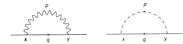
Refer to caption — Figure 1: One-loop contribution to the fermion kinetic term from gauge boson and scalars

For simplicity let us take $\chi=0$ . The fermion propagator receives 1-loop contribution from the Feynman diagrams in figure 1 and figure 2. Both diagrams are planar. For figure 1, summing over the contributions from the gauge and scalar fields, we have

$\displaystyle I_{1}$	$\displaystyle=$	$\displaystyle N\int d^{4}xd^{4}y{\rm Tr}ig_{{\mbox{\tiny YM}}}(x^{+})\bar{\lambda}(x)\Gamma^{M}D(x-y)\Gamma^{N}ig_{{\mbox{\tiny YM}}}(y^{+})\lambda(y)K_{MN}(x-y)$	(77)
	$\displaystyle=$	$\displaystyle 8N\int d^{4}xd^{4}y\frac{d^{4}pd^{4}q}{(2\pi)^{8}}{\rm Tr}g_{{\mbox{\tiny YM}}}(x^{+})\bar{\lambda}(x)\frac{q\hskip-5.29999pt/\hskip 1.49994pt}{p^{2}q^{2}}g_{{\mbox{\tiny YM}}}(y^{+})\lambda(y)e^{i(p+q)(x-y)}$
	$\displaystyle=$	$\displaystyle 4N\int d^{4}xd^{4}y\frac{d^{4}p}{(2\pi)^{4}}{\rm Tr}g_{{\mbox{\tiny YM}}}(x^{+})\bar{\lambda}(x)F(p){p\hskip-6.4pt/\penalty}\;g(y^{+})\lambda(y)e^{ip(x-y)},$

where we have used $\Gamma^{M}q\hskip-5.29999pt/\hskip 1.49994pt\Gamma_{M}=-8q\hskip-5.29999pt/\hskip 1.49994pt$ in the second step, performed a change of variables $q\to q+p/2,p\to-q+p/2$ in the third step, and introduced the definition

F(p):=\int\frac{d^{4}q}{(2\pi)^{4}}\frac{1}{(q-p/2)^{2}(q+p/2)^{2}}.

(78)

To simplify further, we note that

	$\displaystyle\int d^{4}xd^{4}y\int\frac{d^{4}p}{(2\pi)^{4}}f_{1}(x)F(p){p\hskip-6.4pt/\penalty}\;e^{ip(x-y)}f_{2}(y)$
	$\displaystyle=\int d^{4}xd^{4}yf_{1}(x)\bigl(F(i\partial_{y})\cdot i{\partial\hskip-6.4pt/\penalty}\;_{y}\delta(x-y)\bigr)f_{2}(y)$
	$\displaystyle=\int d^{4}xf_{1}(x)F(-i\partial)\cdot(-i{\partial\hskip-6.4pt/\penalty}\;)f_{2}(x)+\int d^{4}xF(i\partial)\cdot i\partial_{\mu}\bigl(f_{1}(x)\Gamma^{\mu}f_{2}(x)\bigr),$		(79)

where $f_{1}=g_{{\mbox{\tiny YM}}}(x^{+})\bar{\lambda}(x)$ and $f_{2}=g_{{\mbox{\tiny YM}}}(x^{+})\lambda(x)$ and we have performed an integration by parts in the last step. The last term above vanishes since $\Gamma^{0}\Gamma^{\mu}$ is symmetric in the Majorana representation. Therefore we obtain

I_{1}=-4N\int d^{4}x{\rm Tr}g_{{\mbox{\tiny YM}}}(x^{+})\bar{\lambda}(x)F(-i\partial)i{\partial\hskip-6.4pt/\penalty}\;\bigl(g_{{\mbox{\tiny YM}}}(x^{+})\lambda(x)\bigr).

(80)

Now the equation of motion has $i{\partial\hskip-6.4pt/\penalty}\;\lambda=$ quadratic in fields, therefore ${\partial\hskip-6.4pt/\penalty}\;\lambda$ can be treated as zero for the fermion kinetic term we are computing. As a result, $I_{1}$ simplifies to

I_{1}=-4N\int d^{4}x{\rm Tr}g_{{\mbox{\tiny YM}}}(x^{+})\bar{\lambda}(x)F(-i\partial)\bigl(i\Gamma^{+}g_{{\mbox{\tiny YM}}}^{\prime}\lambda(x)\bigr).

(81)

The second source of contribution comes from the ${\cal A}_{-}^{2}$ vertex from (60). There is only one diagram (figure 2) since only one such insertion can be made. We have

$\displaystyle I_{2}$	$\displaystyle=$	$\displaystyle N\int d^{4}xd^{4}yd^{4}z{\rm Tr}ig_{{\mbox{\tiny YM}}}(x^{+})\bar{\lambda}(x)\Gamma^{+}D(x-y)\Gamma^{+}ig_{{\mbox{\tiny YM}}}(y^{+})\lambda(y)K_{+-}(x-z)2i\tilde{a}(z^{+})K_{+-}(z-y)$	(82)
	$\displaystyle=$	$\displaystyle 4N\int d^{4}xd^{4}yd^{4}z\frac{d^{4}pd^{4}qd^{4}k}{(2\pi)^{12}}{\rm Tr}g_{{\mbox{\tiny YM}}}(x^{+})\bar{\lambda}(x)\Gamma^{+}\frac{q_{-}}{q^{2}p^{2}k^{2}}g_{{\mbox{\tiny YM}}}(y^{+})\lambda(y)\tilde{a}(z^{+})e^{iq(x-y)}e^{ip(x-z)}e^{ik(z-y)}$
	$\displaystyle=$	$\displaystyle 4N\int d^{4}xd^{4}yd^{4}z\frac{d^{4}pd^{4}k}{(2\pi)^{12}}{\rm Tr}g_{{\mbox{\tiny YM}}}(x^{+})\bar{\lambda}(x)\Gamma^{+}G(p,k)g_{{\mbox{\tiny YM}}}(y^{+})\lambda(y)\tilde{a}(z^{+})e^{ip(x-y)}e^{ik(z-y)},$

where, in the last step, we have shifted the momenta as $q\to q+p/2,p\to-q+p/2,k\to k-q+p/2$ and introduced the kernel

G(p,k):=\int\frac{d^{4}q}{(2\pi)^{4}}\frac{(q+p/2)_{-}}{(q+p/2)^{2}(q-p/2)^{2}(k-q+p/2)^{2}}.

(83)

By performing a similar manipulation like the one above for $I_{1}$ , we finally arrive at

I_{2}=4N\int d^{4}y{\rm Tr}\Bigl(G(i\partial_{x},i\partial_{z})g_{{\mbox{\tiny YM}}}(x^{+})\bar{\lambda}(x)\Gamma^{+}\tilde{a}(z^{+})\Bigr)\Big|_{x=z=y}g_{{\mbox{\tiny YM}}}(y^{+})\lambda(y).

(84)

The effective action is given by the sum $I_{1}+I_{2}$ and is governed by the behaviour of the kernels $F(p),G(p,k)$ given in (78) and (83).

Now, to obtain the Wilsonian effective action, one would like to integrate out oscillation modes with momentum above a cutoff scale $\Lambda$ and replace their contribution to low momentum modes by introducing new interaction vertices in the effective action. However, although the separation of modes is well defined for theory with only global symmetries, the separation into low and high momentum modes does not respect gauge symmetry and hence is not a well-defined procedure. The subtleties concerned with the definition of Wilsonian action for gauge theory were recently discussed in [22]. Instead of using a separation of momentum modes into low and high frequency ones, [22] proposes an alternative procedure by separating the loop momentum into low and high region. In general, the Wilsonian action obtained in this manner contains non-gauge invariant terms. Moreover since one can always shift the loop momentum, one needs to give a specific prescription to avoid any ambiguities. For the 1-loop case, the proposed prescription is, by utilizing the Feynman parametrization, to first reduce the one-loop integral into a certain standard form where there is no linear dependence in the loop momentum in the denominator. Then a IR cutoff on the loop momentum is imposed on this integral. And it has been shown that all non-gauge invariant terms cancel in the case of supersymmetric gauge theories [22].

We remark that in general one may use other prescription to impose a Wilsonian cutoff. This corresponds to different definitions of the Wilsonian effective action which are equivalent in the following sense: the cutoff $\Lambda$ is introduced as an infrared cutoff when computing the Wilsonian action. It becomes a UV cutoff when one uses the Wilsonian action to compute correlation functions. Although one may obtain different Wilsonian actions with different ways to impose the IR cutoff, as long as one uses the same corresponding prescription for the UV cutoff, one will get the same correlation functions when using the Wilsonian action to compute correlators.

Now let us introduce the Wilsonian cutoff following the above prescription. The kernels with high loop momenta modes integrated out are given by

F_{W}(p):=\int_{0}^{1}d\alpha\int_{\Lambda}^{\infty}\frac{d^{4}q}{(2\pi)^{4}}\frac{1}{\bigl(q^{2}+\alpha(1-\alpha)p^{2}\bigr)^{2}},

(85)

G_{W}(p,k):=2\int_{0}^{1}d\alpha_{1}d\alpha_{2}d\alpha_{3}\int_{\Lambda}^{\infty}\frac{d^{4}q}{(2\pi)^{4}}\frac{\delta(\alpha_{1}+\alpha_{2}+\alpha_{3}-1)[(1-\alpha_{1})p_{-}+\alpha_{3}k_{-}]}{\bigl(q^{2}+\alpha_{1}(1-\alpha_{1})p^{2}+\alpha_{3}(1-\alpha_{3})k^{2}+2\alpha_{1}\alpha_{3}p\cdot k\bigr)^{3}}.

(86)

As noted above, their contributions to low momentum modes then appear as new interaction vertices in the Wilsonian action.

The kernels $F_{W},G_{W}$ can be evaluated and give an expansion of the Wilsonian action in derivatives of the field $\lambda$ . Let us first start with $I_{1}$ . It is straightforward to compute $F_{W}$ and we have

	$\displaystyle F_{W}(p)$	$\displaystyle=$	$\displaystyle\frac{1}{16\pi^{2}}\left[C+1-\frac{4+2y}{\sqrt{(4+y)y}}\sinh^{-1}(\frac{\sqrt{y}}{2})\right],\qquad y:=p^{2}/\Lambda^{2},$		(87)
		$\displaystyle=$	$\displaystyle\frac{C}{16\pi^{2}}+\sum_{n=1}^{\infty}\frac{(n-1)!(n+1)!}{(2n+1)!}\left(\frac{-p^{2}}{\Lambda^{2}}\right)^{n},$		(87)

where $C=\log s|_{\Lambda^{2}}^{\infty}$ is an infinite constant. This does not contribute to (81). Using $-p^{2}=\partial^{2}=-2\partial_{-}\partial_{+}+\partial_{i}^{2}$ , it is easy to find

I_{1}=\frac{iN}{6\pi^{2}\Lambda^{2}}\int d^{4}xg_{{\mbox{\tiny YM}}}^{\prime 2}{\rm Tr}\bar{\lambda}\Gamma^{+}\partial^{+}\lambda+\cdots,

(88)

where $\cdots$ are terms of second or higher derivatives of $\lambda$ . We have kept only terms which are first order in derivatives of $\lambda$ since, as we will see in the next subsection, these terms may be interpreted as due to a nonzero component $g_{++}$ of the metric.

As for $I_{2}$ , it is easy to evaluate the $q$ -integral and get

	$\displaystyle G_{W}(p,k)$	$\displaystyle=$	$\displaystyle\frac{1}{16\pi^{2}}\int_{0}^{1}d\alpha_{1}\int_{0}^{1-\alpha_{1}}d\alpha_{3}[(1-\alpha_{1})p_{-}+\alpha_{3}k_{-}]\frac{\Delta+2\Lambda^{2}}{(\Delta+\Lambda^{2})^{2}}$		(89)
		$\displaystyle=$	$\displaystyle\frac{1}{8\pi^{2}}\left[\frac{p_{-}}{3\Lambda^{2}}-\frac{(6p^{2}+6p\cdot k+7k^{2})p_{-}}{80\Lambda^{4}}+\cdots\right],$		(89)

where $\Delta=\alpha_{1}(1-\alpha_{1})p^{2}+\alpha_{3}(1-\alpha_{3})k^{2}+2\alpha_{1}\alpha_{3}p\cdot k$ , as an momentum expansion. We have dropped the $k_{-}$ term in the last line above since $k_{-}=0$ when acting on a function of $z^{+}$ and hence this term does not contribute in (84). Substituting (89) into (84), we obtain

I_{2}=\frac{iN}{3\pi^{2}\Lambda^{2}}\int d^{4}xg_{{\mbox{\tiny YM}}}^{\prime 2}{\rm Tr}\bar{\lambda}\Gamma^{+}\partial^{+}\lambda+\cdots,

(90)

where, again, $\cdots$ denotes terms of second or higher derivatives of $\lambda$ .

Concentrating on the first derivative terms, we find the 1-loop Wilsonian action $\Gamma_{\rm eff,1}=I_{1}+I_{2}$ ,

\Gamma_{\rm eff,1}=\frac{iN}{2\pi^{2}\Lambda^{2}}\int d^{4}xg_{{\mbox{\tiny YM}}}^{\prime 2}{\rm Tr}\bar{\lambda}\gamma^{+}\partial^{+}\lambda.

(91)

Substituting $g_{{\mbox{\tiny YM}}}^{2}=4\pi e^{\phi}$ , we finally obtain

\Gamma_{\rm eff,1}\approx i\int d^{4}x\frac{Ne^{\phi}}{2\pi\Lambda^{2}}{\phi^{\prime}}^{2}{\rm Tr}\bar{\lambda}\Gamma^{+}\partial^{+}\lambda.

(92)

5.2 Holographic reconstruction of bulk metric

Next we want to find an interpretation of the result (92) which will allow us to reconstruct the bulk metric. We start by noting that two different UV/IR relations have been considered [18]. In terms of our coordinates, these are

	$\displaystyle u$	$\displaystyle\sim$	$\displaystyle\frac{1}{\Lambda},$		(93)
	$\displaystyle u$	$\displaystyle\sim$	$\displaystyle\frac{g_{{\mbox{\tiny YM}}}N^{1/2}}{\Lambda}.$		(94)

In the original $AdS_{5}\times S^{5}$ case, the two relations are similar except for an overall constant which depends on the gauge coupling. The holographic relation (93) corresponds to a probe by one of the massless supergravity fields and can be derived by a scaling argument for the wave equation in the SUGRA background. This relation has been applied to the counting of entropy [17]. The holographic relation (94) is relevant for the effective action of a D3-brane probe at a distance $u$ and is derived by a stretched open string attached to the D3-brane.

In our case with a time dependent coupling $g_{{\mbox{\tiny YM}}}$ , the two relations are distinctly different. If we employ the holographic relation (94), but more precisely:

u=\frac{g_{{\mbox{\tiny YM}}}(x^{+})N^{1/2}}{\Lambda}\frac{1}{\pi},

(95)

then the effective action (92) can be written as

\Gamma_{\rm eff,1}\approx i\int d^{4}x\;\frac{u^{2}}{8}{\phi^{\prime}}^{2}{\rm Tr}\bar{\lambda}\Gamma^{+}\partial^{+}\lambda.

(96)

Compared to (94), eq.(95) includes an additional numerical factor of $\pi$ . We remark that previous tests of the holographic relation is not sensitive to the overall numerical factor. Here it is fixed by requiring a matching with the bulk metric as we will demonstrate.

Next let us compute the kinetic term for the fermion field for D3 branes placed at $u$ of (95). Normally a D3 brane sitting at a constant $u$ is 1/2 BPS. It is quite remarkable that for our supergravity background, a D3-brane sitting at an arbitrary $u=u(x^{+})$ is also 1/2 BPS. To see this, consider the action for a D3-brane probe with zero worldvolume field strength,

I=\int d^{4}xe^{-\phi}\sqrt{-\det G_{\mu\nu}}+\int C,

(97)

where

G_{\mu\nu}=\frac{\partial X^{M}}{\partial x^{\mu}}\frac{\partial X^{N}}{\partial x^{\nu}}g^{(s)}_{MN}

(98)

is the pull back to D3-brane worldvolume of the spacetime metric in the string frame $g^{(s)}_{MN}=e^{\phi/2}g_{MN}$ and $g_{MN}$ is given by (34). For a D3-brane in the static gauge $X^{\mu}=x^{\mu}$ , $\mu=+,-,2,3$ and with $u=u(x^{+})$ , it is

G_{\mu\nu}=\frac{e^{\phi/2}}{u^{2}}(\eta_{\mu\nu}+\frac{\Omega}{2}u^{2}\delta_{\mu+}\delta_{\nu+}).

(99)

It is easy to check that the variation of the Born-Infeld term $\delta I_{0}/\delta u$ cancels against the variation $\delta I_{WZ}/\delta u$ of the WZ term. The equation of motion for $u$ is thus

\partial_{\mu}\frac{\delta I_{0}}{\delta(\partial_{\mu}u)}=\partial_{\mu}\bigl(\frac{\sqrt{-G}}{u^{2}}(G^{-1})^{\mu\nu}\partial_{\nu}u\bigr)=0,

(100)

which is satisfied for arbitrary $u(x^{+})$ since $(G^{-1})^{++}=0$ . As for supersymmetry, the preserved supersymmetry is given by the kappa-symmetry condition

(1-\Gamma)\epsilon=0,

(101)

where

\Gamma=\frac{-i}{4!\sqrt{-G}}\epsilon^{\mu_{1}\cdots\mu_{4}}\partial_{\mu_{1}}X^{M_{1}}\cdots\partial_{\mu_{4}}X^{M_{4}}\Gamma^{\prime}_{M_{1}\cdots M_{4}},

(102)

\Gamma^{\prime}_{M}=E_{M}^{A}\Gamma_{A}

(103)

and $\Gamma_{A}$ are the flat space $\Gamma$ -matrices. $\epsilon$ has to satisfy also the condition (15) of the II B supergravity background. For our D3-brane, it is easy to obtain

\Gamma=-i(\Gamma^{23}+\Gamma^{23-+}-u^{\prime}\Gamma^{23r+}).

(104)

Using $\Gamma^{+}\epsilon=0$ , this reduces to $\Gamma=-i\Gamma^{23}$ . Thus we conclude that the D3-brane is supersymmetric for the SUSY parameter satisfying the projector conditions (15) and $(1-i\Gamma^{23})\epsilon=0$ .

For such a D3 brane, the bulk metric (34) at nonzero $u(x^{+})$ gets an additional contribution and the induced metric (apart from the factor $R^{2}/u^{2}$ ) is

ds^{2}_{4D}=-2dx^{+}dx^{-}+dx_{i}^{2}+\left(\frac{1}{4}\phi^{\prime}{}^{2}+u^{\prime 2}/u^{2}\right)u^{2}dx^{+}{}^{2}:=\eta_{\mu\nu}dx^{\mu}dx^{\nu}+\hat{g}_{++}dx^{+}{}^{2}.

(105)

The curved space gamma matrices $\gamma_{\mu}$ are related to the flat space ones by

\gamma^{-}=\Gamma^{-}+\frac{1}{2}\hat{g}_{++}\Gamma^{+},\quad\gamma^{+}=\Gamma^{+},\quad\gamma_{i}=\Gamma_{i}.

(106)

Therefore among other terms, there will be a kinetic term for the fermion:

-\frac{i}{2}\bar{\lambda}\gamma^{\mu}\partial_{\mu}\lambda=-\frac{i}{2}\bar{\lambda}\Gamma^{a}\partial_{a}\lambda+\frac{i}{4}\hat{g}_{++}\bar{\lambda}\Gamma^{+}\partial^{+}\lambda.

(107)

And we expect an additional term

\frac{i}{4}\int d^{4}x\,\hat{g}_{++}{\rm Tr}\bar{\lambda}\Gamma^{+}\partial^{+}\lambda=i\int d^{4}x\,\frac{u^{2}}{8}\left(\frac{1}{2}\phi^{\prime 2}+2u^{\prime 2}/u^{2}\right){\rm Tr}\bar{\lambda}\Gamma^{+}\partial^{+}\lambda

(108)

in the kinetic action of $\lambda$ in addition to the kinetic term for flat space. Using the UV/IR relation (95), this is precisely equal to (96).

Thus we observe that the fermion kinetic term in the one-loop Wilsonian action seems to know about the bulk metric. A priori, the 1-loop correction may be more general than being equivalent to turning on the $\hat{g}_{++}$ component of the metric. In addition, the functional form of the $\hat{g}_{++}$ component is precisely reproduced. In general, the D3-brane probe action cannot be identified with the Wilsonian action at the scale (94). However, sometimes there is supersymmetry protecting certain loop amplitudes [18]. In particular it seems to be the case for the kinetic term of the Wilsonian effective action. This leads us to the proposal to identify the metric of bulk spacetime from the kinetic term of the Wilsonian action.

More explicitly, we are proposing a relation between the metric derived from the Wilsonian action and the induced metric in the D3-brane probe action

g^{\rm(YM)}_{MN}(\lambda,g_{s})=g^{\rm(Bulk)}_{MN}(\lambda,g_{s}),\qquad M,N=+,-,2,3,u.

(109)

In general, the metric on the left hand side is valid only when ’t Hooft’s coupling is small, while the quantity on the right hand side is good only when ’t Hooft’s coupling is large. Our conjecture is that this relation is protected by supersymmetry.

As remarked above, the form of the Wilsonian action is generally dependent on the scheme implementing the infrared cutoff. An immediate problem arises if one would like to propose it to be in correspondence with bulk gravitational physics since the latter, at least the bulk geometry, should be independent of any particular cutoff scheme. In the above, if we have shifted the loop momenta and then impose the cutoff, this will lead to a different coefficient, in the $1/\Lambda$ expansion, for the $p^{2}/\Lambda^{2}$ term of $F(p)$ and for the $p_{-}/\Lambda^{2}$ term of $G(p,k)$ . This has the effect of changing the overall coefficient of the effective action $\Gamma_{\rm eff,1}$ (92). However this will only result in a modification to the formula (95) which matches $u$ with $\Lambda$ by an overall constant. Thus one can always reproduce the bulk metric from the Wilsonian effective action of SYM.

Strictly speaking, it is not clear to what extent the supersymmetry can protect loop correction in matching D3-probe action with the Wilsonian effective action of the boundary SYM. Let us recall that while the $v^{4}$ term of SUGRA scattering amplitude is correctly reproduced in field theory [21], higher momentum dependence is not [20]. We showed above that the lowest derivative terms fixed by the bulk metric (108) are correctly reproduced. In the effective action there are terms involving higher derivatives of $\lambda$ . It is not difficult to include these higher order contributions. It remains to be seen whether and how these terms in the Wilsonian effective action correspond to quantum effects on the gravity side.

A similar calculation may be performed at higher loops. For example, the metric component $\hat{g}_{++}$ we calculated above will be modified. Generally it takes the form:

\hat{g}_{++}=a(\phi,u^{2})(\phi^{\prime})^{2},

(110)

where we have used the UV/IR relation to replace the $1/\Lambda^{2}$ depenence with $u$ -dependence. Higher loop amplitudes contribute higher order in powers of $g_{{\mbox{\tiny YM}}}$ , but only a $(\phi^{\prime})^{2}$ dependence. In general, following the above procedue, the higher loop corrections in gauge theory gives a 5d metric:

ds^{2}=\frac{R^{2}}{u^{2}}(g^{\rm(YM)}_{\mu\nu}(u,x^{+})dx^{\mu}dx^{\nu}+du^{2}).

(111)

Due to the complicated $u$ -dependence, the metric will generally not satisfy the Einstein equation. The dual supersymmetric Yang-Mills provides a framework for computing the quantum corrections to the supergravity action. This includes higher derivatives corrections in general. It will be very interesting to see if one is able to reproduce some of the well-known result, e.g. the $R^{4}$ term [23], from the SYM theory.

5.3 On resolution of spacetime singularity

The above analysis is performed for a correspondence which is defined over the whole real line of $x^{+}$ . In case when the SUGRA background is singular, say at $x^{+}=0$ , the SUGRA solution in the two regions $x^{+}>0$ and $x^{+}<0$ are actually two different solutions as, at least classically, the degrees of freedom don’t talk to each other. A possibility is that the SUGRA solution restricted to, say $x^{+}>0$ , should be matched with the dual SYM constructed on $x^{+}>0$ ⁴⁴ 4 The Feynman rules will become more complicated. Principal value appears in (73) and (74) in addition to the Dirac delta function. . However, it is also possible that stringy or quantum corrections to the SUGRA solution will resolve the singularity, and both regions must be included in the complete theory. The dual SYM theory will then be defined on the whole real line of $x^{+}$ . In particular, when the SUGRA singularity corresponds to the vanishing of the YM coupling at $x^{+}=0$ , the dual SYM theory is weakly coupled around the point $x^{+}=0$ , and has no reason to break down. What happens in the bulk must be that the stringy and/or quantum corrections resolve the SUGRA singularity

We will now argue that the second possibility is the generic scenario, whenever the dual SYM theory is well defined. Despite the fact the two regions are separated by the singularity, one may still put the two halves of the SUGRA background together and consider the total theory $S=S_{1}+S_{2}$ , where $S_{1}$ or $S_{2}$ describes the SUGRA on $x^{+}>0$ or $x^{+}<0$ respectively. The dual SYM is now defined on the whole $x^{+}$ and the Feynman rules take on the simple form as described before. In this description, SUGRA restricted to one of the two regions can be described as a subsector of the SYM theory.

Classically, $S_{1}$ and $S_{2}$ don’t interact with each other. However, in the SYM, the replacement of principal value by delta function in the Feynman rules means something nontrivial must happen. From the result of the previous subsection, we see that the singular metric is reproduced by the SYM at the 1-loop level. Taking into account of the corrections from higher loops, the dual bulk metric becomes (111). It is possible that the metric becomes regular after taking into account of these higher order corrections. A rather generic argument supports that spacetime singularity is indeed resolved. In the Wilsonian effective action, since oscillations of frequency above an energy scale $\Lambda$ are integrated out, the higher derivative correction to the kinetic term must be such that the background geometry is smeared over a length scale of $\Delta x\sim 1/\Lambda$ . A potential singularity in $g_{++}$ is thus always resolved for any finite $\Lambda$ . It will be very interesting to check explicitly if this is really the case.

6 Discussions

In our perturbative analysis above we have turned off the axion coupling ( $\chi^{\prime}=0$ ) for simplicity. Since both type II B SUGRA and ${\cal N}=4$ SYM have the $SL(2,\mathbb{Z})$ symmetry [24] which mixes the dilaton and axion fields

\tau=\chi+ie^{-\phi}\rightarrow\tau^{\prime}=\frac{a\tau+b}{c\tau+d},

(112)

the extension of our results to a nontrivial axion field background should presumably be a direct result of the $SL(2,\mathbb{Z})$ symmetry, assuming that there is no technical difficulty in manifestly preserving this symmetry, as well as gauge symmetry and supersymmetry in the Wilsonian effective action.

We have shown in this paper that the spacetime metric can be holographically reconstructed from the kinetic term of the SYM Wilsonian effective action in the leading order approximation. Higher order corrections to the kinetic term of the Wilsonian action include quantum corrections (both $\alpha^{\prime}$ and $g_{s}$ ) to the SUGRA equations of motion. Due to the nature of the Wilsonian action where high momentum modes are integrated out, it is expected that singularity in the metric will be resolved. The confirmation of this will be very interesting.

We remark that in the matrix cosmology proposal [13, 25], it has been suggested that as one approaches the singularity, the classical picture of spacetime breaks down since the non-diagonal degrees of freedom of the matrix model get lighter and lighter and their effects cannot be ignored, and that the singularity could be resolved by including these light modes in the description. Doing so, spacetime is replaced by nonabelian matrices. Our proposal is different. In our proposal, we have suggested a mechanism how spacetime singularity could be resolved by including all the quantum corrections to the Einstein equation, which in principle could be computed from the gauge theory. After the resolution, ordinary spacetime is still a valid concept. However, without understanding the nature and organization principle of these corrections, one does not actually feel one has a good understanding of the physics involved. It is usually believed that some form of quantized spacetime and noncommutative geometry will be relevant at very small distance scale. In the case of noncommutative quantum field theory, one way to think about the noncommutative geometry is that it is an effective and geometrical way to encode the Moyal phase factor. It may be possible that the infinite series of quantum corrections follows from some form of underlying noncommutative geometry. If this really happens, the noncommutative geometry description will be a better one than the classical spacetime. It is interesting to explore this possibility.

Acknowledgements

We thank Ed Corrigan, Nick Dorey, Harald Dorn, Chris Fewster, Kazuyuki Furuuchi, Jerome Gauntlett, Hsien-Chung Kao, James Liu, Kelly Stelle, Takeo Inami, Shunsuke Teraguchi, Wen-Yu Wen, Toby Wiseman, Tamiaki Yoneya and Syoji Zeze for valuable discussions. CSC also thanks the Isaac Newton Institute for Mathematical Sciences for hospitality, and participants of the programme ”Strong Fields, Integrability and Strings” for discussions. The work of CSC is supported in part by EPSRC and PPARC. The work of PMH is supported in part by the National Science Council, and the National Center for Theoretical Sciences, Taiwan, R.O.C.

References

[1] T. Banks, W. Fischler, S. H. Shenker and L. Susskind, “M theory as a matrix model: A conjecture,” Phys. Rev. D 55 (1997) 5112 [arXiv:hep-th/9610043].
[2] D. Bigatti and L. Susskind, “Review of matrix theory,” arXiv:hep-th/9712072.
T. Banks, “TASI lectures on matrix theory,” arXiv:hep-th/9911068.
W. Taylor, “M(atrix) theory: Matrix quantum mechanics as a fundamental theory,” Rev. Mod. Phys. 73 (2001) 419 [arXiv:hep-th/0101126].
[3] J. M. Maldacena, “The large N limit of superconformal field theories and supergravity,” Adv. Theor. Math. Phys. 2 (1998) 231 [Int. J. Theor. Phys. 38 (1999) 1113] [arXiv:hep-th/9711200].
[4] S. S. Gubser, I. R. Klebanov and A. M. Polyakov, “Gauge theory correlators from non-critical string theory,” Phys. Lett. B 428 (1998) 105 [arXiv:hep-th/9802109].
[5] E. Witten, “Anti-de Sitter space and holography,” Adv. Theor. Math. Phys. 2 (1998) 253 [arXiv:hep-th/9802150].
[6] O. Aharony, S. S. Gubser, J. M. Maldacena, H. Ooguri and Y. Oz, “Large N field theories, string theory and gravity,” Phys. Rept. 323, 183 (2000) [arXiv:hep-th/9905111].
E. D’Hoker and D. Z. Freedman, “Supersymmetric gauge theories and the AdS/CFT correspondence,” arXiv:hep-th/0201253.
[7] V. Balasubramanian and S. F. Ross, “Holographic particle detection,” Phys. Rev. D 61 (2000) 044007 [arXiv:hep-th/9906226].
J. Louko, D. Marolf and S. F. Ross, “On geodesic propagators and black hole holography,” Phys. Rev. D 62 (2000) 044041 [arXiv:hep-th/0002111].
J. M. Maldacena, “Eternal black holes in Anti-de-Sitter,” JHEP 0304 (2003) 021 [arXiv:hep-th/0106112].
P. Kraus, H. Ooguri and S. Shenker, “Inside the horizon with AdS/CFT,” Phys. Rev. D 67 (2003) 124022 [arXiv:hep-th/0212277].
L. Fidkowski, V. Hubeny, M. Kleban and S. Shenker, “The black hole singularity in AdS/CFT,” JHEP 0402 (2004) 014 [arXiv:hep-th/0306170].
[8] L. Cornalba and M. S. Costa “Time-dependent orbifolds and string cosmology,” Fortsch. Phys. 52, 145 (2004) [arXiv:hep-th/0310099].
B. Craps, “Big bang models in string theory,” Class. Quant. Grav. 23 (2006) S849 [arXiv:hep-th/0605199].
M. Berkooz and D. Reichmann, “A short review of time dependent solutions and space-like singularities in string theory,” Nucl. Phys. Proc. Suppl. 171 (2007) 69 [arXiv:0705.2146 [hep-th]].
S. R. Das, “Holography and Cosmological Singularities,” [arXiv:0706.4188 [hep-th]].
[9] C.S. Chu and P.M. Ho, “ Time-dependent AdS/CFT Duality and Null Singularity”, [hep-th/0602054].
[10] F. L. Lin and W. Y. Wen, “Supersymmteric null-like holographic cosmologies,” JHEP 0605 (2006) 013 [arXiv:hep-th/0602124].
[11] S. R. Das, J. Michelson, K. Narayan and S. P. Trivedi, “Time dependent cosmologies and their duals,” Phys. Rev. D 74 (2006) 026002 [arXiv:hep-th/0602107].
[12] T. Hertog and G. T. Horowitz, “Towards a big crunch dual,” JHEP 0407, 073 (2004) [arXiv:hep-th/0406134].
T. Hertog and G. T. Horowitz, “Holographic description of AdS cosmologies,” JHEP 0504, 005 (2005) [arXiv:hep-th/0503071].
[13] B. Craps, S. Sethi and E. P. Verlinde, “A matrix big bang,” arXiv:hep-th/0506180.
[14] M. Cvetic, S. Nojiri and S. D. Odintsov, “Cosmological anti-de Sitter space-times and time-dependent AdS/CFT correspondence,” Phys. Rev. D 69, 023513 (2004) [arXiv:hep-th/0306031].
[15] M. Li, “A class of cosmological matrix models,” arXiv:hep-th/0506260.
B. Chen, “The time-dependent supersymmetric configurations in M-theory and matrix models,” arXiv:hep-th/0508191.
J. H. She, “A matrix model for Misner universe,” arXiv:hep-th/0509067.
T. Ishino, H. Kodama and N. Ohta, “Time-dependent solutions with null Killing spinor in M-theory and superstrings,” Phys. Lett. B 631 (2005) 68 [arXiv:hep-th/0509173].
D. Robbins and S. Sethi, “A matrix model for the null-brane,” arXiv:hep-th/0509204.
M. Li and W. Song, “A one loop problem of the matrix big bang model,” JHEP 0608, 089 (2006) [arXiv:hep-th/0512335].
B. Craps, A. Rajaraman and S. Sethi, “Effective dynamics of the matrix big bang,” Phys. Rev. D 73 (2006) 106005 [arXiv:hep-th/0601062].
T. Ishino and N. Ohta, “Matrix string description of cosmic singularities in a class of time-dependent solutions,” Phys. Lett. B 638 (2006) 105 [arXiv:hep-th/0603215].
F. L. Lin and D. Tomino, “One-loop effect of null-like cosmology’s holographic dual super-Yang-Mills,” JHEP 0703, 118 (2007) [arXiv:hep-th/0611139].
[16] S. R. Das, J. Michelson, K. Narayan and S. P. Trivedi, “Cosmologies with null singularities and their gauge theory duals,” Phys. Rev. D 75 (2007) 026002 [arXiv:hep-th/0610053].
[17] L. Susskind and E. Witten, “The holographic bound in anti-de Sitter space,” arXiv:hep-th/9805114.
[18] A. W. Peet and J. Polchinski, “UV/IR relations in AdS dynamics,” Phys. Rev. D 59 (1999) 065011 [arXiv:hep-th/9809022].
[19] S. de Haro, S. N. Solodukhin and K. Skenderis, “Holographic reconstruction of spacetime and renormalization in the AdS/CFT correspondence,” Commun. Math. Phys. 217, 595 (2001) [arXiv:hep-th/0002230].
J. de Boer, E. P. Verlinde and H. L. Verlinde, “On the holographic renormalization group,” JHEP 0008, 003 (2000) [arXiv:hep-th/9912012].
K. Skenderis, “Lecture notes on holographic renormalization,” Class. Quant. Grav. 19 (2002) 5849 [arXiv:hep-th/0209067].
[20] M. R. Douglas and W. I. Taylor, “Branes in the bulk of anti-de Sitter space,” arXiv:hep-th/9807225.
[21] M. R. Douglas, D. Kabat, P. Pouliot and S. H. Shenker, “D-branes and short distances in string theory,” Nucl. Phys. B 485, 85 (1997) [arXiv:hep-th/9608024].
[22] A. Bilal, “(Non) Gauge Invariance of Wilsonian Effective Actions in (Supersymmetric) Gauge Theories : A Critical Discussion,” arXiv:0705.0362 [hep-th].
[23] M. B. Green and M. Gutperle, “Effects of D-instantons,” Nucl. Phys. B 498 (1997) 195 [arXiv:hep-th/9701093].
M. B. Green and S. Sethi, “Supersymmetry constraints on type IIB supergravity,” Phys. Rev. D 59 (1999) 046006 [arXiv:hep-th/9808061].
[24] A. Sen, “Dyon - monopole bound states, selfdual harmonic forms on the multi - monopole moduli space, and SL(2,Z) invariance in string theory,” Phys. Lett. B 329, 217 (1994) [arXiv:hep-th/9402032]; C. Vafa and E. Witten, “A Strong coupling test of S duality,” Nucl. Phys. B 431, 3 (1994) [arXiv:hep-th/9408074].
[25] M. Li and W. Song, “Shock waves and cosmological matrix models,” arXiv:hep-th/0507185.