Efficient Skyline Querying with Variable User Preferences on Nominal Attributes
Abstract
Current skyline evaluation techniques assume a fixed ordering on the attributes. However, dynamic preferences on nominal attributes are more realistic in known applications. In order to generate online response for any such preference issued by a user, we propose two methods of different characteristics. The first one is a semi-materialization method and the second is an adaptive SFS method. Finally, we conduct experiments to show the efficiency of our proposed algorithms.
1 Introduction
The skyline operator has emerged as an important summarization technique for multi-dimensional datasets. Given a set of -dimensional data points, the skyline is the set of all points such that there is no other point which dominates . is said to dominate if is better than in at least one dimension and not worse than in all other dimensions. Consider a customer looking for a vacation package to Cancun using three criteria: price, hotel-class and number of stops. We know that lower price, higher hotel class and less stops are more preferable. Thus, if is in the skyline, then there is no other package which has lower price, higher hotel class and less stops compared with .
Skyline queries have been studied since 1960s in the theory field where skyline points are known as Pareto sets and admissible points [10] or maximal vectors [9]. However, earlier algorithms such as [9, 8] are inefficient when there are many data points in a high dimensional space. The problem of skyline queries was introduced in the database context in [1].
Most of the existing studies handle only numeric attributes. Consider an example as shown in Table 2 showing a set of vacation packages with three attributes or dimensions11 1 In this paper, we use the terms “attribute” and “dimension” interchangeably., Price, Hotel-class and Hotel-group. Most existing works consider the first two attributes which are numeric, where lower price and higher hotel-class are more preferable. Many efficient methods have been proposed for so-called full-space skyline queries which return a set of skyline points in a specific space (a set of dimensions such as price and hotel-class). Some representative methods include a block nested loop (BNL) algorithm [1], a sort first skyline (SFS) algorithm [7], a bitmap method [19], a nearest neighbor (NN) algorithm [13] and a branch and bound skylines (BBS) method [14, 15]. Recently, skyline computation has been extended to consider subspace skyline queries which return the skylines in subspaces [23, 17, 22, 18, 16].
|
|
Hotel-group as shown in Table 2 is a categorical attribute. There can be partial ordering on categorical attributes. Some recent studies [3, 2, 4, 6, 5, 12, 11, 20] consider partially-ordered categorical attributes. In [3, 2], each partially-ordered attribute is transformed into two-integer attributes such that the conventional skyline algorithms can be applied. [4] studies the cost estimation of the skyline operator involving the partially ordered attributes.
Nevertheless, known existing work on categorical attributes assumes that each attribute has only one order: either a total or a partial order. In real life, it is not often that categorical attributes have a fixed predefined order. For example, different customers may prefer different realty locations, different car models, or different airlines. We call such a categorical attribute which does not come with a predefined order a nominal attribute. It is easy to name important applications with nominal attributes, such as realties (where type of realty, regions and style are examples of nominal attributes) and flight booking (where airline and transition airport are examples of nominal attributes). In this paper, we consider the scenarios where different users may have different preferences on nominal attributes. That is, more than one order need to be considered in nominal attributes.
Furthermore, typically, for a nominal attribute, there may be many different values, and a user would not specify an order on all the values, but would only list a few of the most favorite choices. Table 2 shows different customer preferences on Hotel-group. The preference of Alice is “” which means that she prefers Tulips to Mozilla and prefers these two to other hotel groups (i.e., Horizon). We call such preferences implicit preferences. Note that different preferences yield different skylines. As shown in Table 2, the skyline is for Alice’s preference but for Fred’s preference. The numerous skylines make the problem highly challenging.
Some latest works [6, 5] study the problem of preference changes, whereupon the query results can be incrementally refined. In [12], a user or a customer can specify some values in nominal attributes as an equivalence class to denote the same “importance” for those values. [11] is an extension of [12]. In [11], whenever a user finds that there are a lot of irrelevant results for a query, s/he can modify the query by adding more conditions so that the result set is smaller to suit her/his need. However, these works only focus either on the effects of the query changes on the result size, or the reuse of skyline results when a query is refined in a progressive manner, but not on finding efficient algorithms. Here, we consider that different users may have different preferences and so the preferences are not undergoing refinement but they can be different or conflicting from one query to another. Also, we focus on the issue of efficient query answering. Nominal attributes are first considered in [20] but there the study is about finding a set of partial orders with respect to which a given point is in the skyline.
In [15], dynamic skyline is considered but it is only for numeric data, and the “dynamic function” considered is based on distance from a user location. Here, we consider nominal attributes, and the “dynamic function” is any mapping between the nominal values and the rankings where each nominal value is assigned with a ranking value. The BBS method does not work in our case.
Our contributions include the following. (1) To the best of our knowledge, this is the first work to study the problem of efficient skyline querying with respect to dynamic implicit preference on nominal attributes. (2) We propose two efficient algorithms of different flavors, namely IPO-Tree Search and Adaptive SFS. IPO-Tree is a partial materialization of the skylines for all possible implicit preferences. It facilitates the efficient computation of the skyline for any implicit preference. Adaptive SFS is a little slower but it does not require materialization and has the nice properties of being progressive and allows for incremental maintenance. (3) We have conducted extensive experiments to show the the efficiency of our proposed algorithms.
2 Problem Definition
A skyline analysis involves multiple attributes. A user’s preference on the values in an attribute can be modeled by a partial order on the attribute. A partial order is a reflexive, asymmetric and transitive relation. A partial order is also a total order if, for any two values and in the domain, either or . We write if and . A partial order also can be written as . also can be written as . We call this model as the partial order model.
By default, we consider points in an -dimensional space . For each dimension , we assume that there is a partial or total order on the values in . For a point , is the projection on dimension . If , we also write .
For points and , dominates , denoted by , if, for any dimension , , and there exists a dimension such that . If dominates , then is more preferable than according to the preference orders. The dominance relation can be viewed as the integration of the preference partial orders on all dimensions. Thus, we can write . It is easy to see that the dominance relation is a strict partial order.
Given a data set containing data points in space , a point is in the skyline of (i.e., a skyline point in ) if is not dominated by any points in . Given a preference , the skyline of , denoted by , is the set of skyline points in .
In many applications, there often exist some orders on some of the dimensions that hold for all users. In our example in Table 2, a lower price and a higher hotel-class are always more preferred by customers. Even for nominal attributes, there may exist some universal partial orders. Hence, we assume that we are given a template, which contains a partial order for every dimension. The partial orders in the template are applicable to all users. Each user can then express his/her specific preference by refining the template. The containment relation of orders captures the refinement.
For partial orders and , is a refinement of , denoted by , if for any , . Moreover, if and , is said to be stronger than . Let and . Then, . That is, is a refinement of by adding a preference . As , is stronger than .
Property 1
For orders and , , , if and only if for .
Theorem 1 (Monotonicity)
([20]) Given a data set and a template , if is not in the skyline with respect to , then is not in the skyline with respect to any refinement of .
Theorem 1 indicates that, when the orders on the dimensions are strengthened, some skyline points may be disqualified. However, a non-skyline point never gains the skyline membership due to a stronger order. This monotonic property greatly helps in analyzing skylines with respect to various orders.
Definition 1 (Conflict-free)
([20]) Let and be two partial orders. and are conflict-free if there exist no values and such that , , and .
Although the model of partial order refinements can model diverse individual preferences, it does not fit tightly the real world scenarios. In a skyline query, for a nominal attribute, users typically would not explicitly order all values, but may specify a few of their favorite choices and also give them an ordering. For example, a user may specify that the first choice is , the second choice is . The implicit meaning is that and are better than all the other choices, say . We can model this by the partial order model, by including , , , …, and , , …, . We denote this preference by “” where means all choices other than and (in this case, corresponds to ). We call this special kind of partial order an implicit preference and assume that it is represented in such a form. For example, the implicit preference “” corresponds to a set of binary orders in the partial order model.
Definition 2 (Implicit Preferences)
Let be all the values in a nominal attribute . An implicit preference on is given by . It is equivalent to the partial order given by .
In the above definition, is said to be an -th order implicit preference. Also, the order of , denoted by , is defined to be and the order of is defined to be . A value is said to be in if . Also, is said to be the -th entry in . is defined to be . Let . is defined to be .
In this paper, we adopt the convention that denotes an implicit preference and denotes a partial order (which may or may not be an implicit preference). Also we denote by .
Definition 3 (Problem)
Given a dataset and an implicit preference , find the skyline in .
The problem defined above is our objective in this paper. We also say that we want to find a set of skyline points with respect to in . In many applications, online response is required. The extensive study in [15] reports that all the existing algorithms have some serious shortcomings and a new algorithm BBS is proposed which is much more efficient than previous methods. However, the data partitioning in BBS is based on fixed orderings on the dimensions and the same partitioning cannot be used for dynamic or variable preferences on nominal attributes. Therefore, new mechanisms need to be explored.
The problem of dynamic implicit preferences have some similar flavor to subspace skylines since materialization of the possible skylines seems to be a solution. However, as noted in [15], most applications involve up to five attributes, the dimensionality of a typical skyline problem is not high, and therefore materialization of the skylines is quite feasible and has been investigated in recent works such as [23, 22, 18, 16]. For dynamic implicit preferences, the number of combinations is exponential not only in the dimensionality but also in the cardinalities of the attributes, which makes the problem much more challenging.
| Package | Price | Hotel-class | Hotel group | Airline |
|---|---|---|---|---|
| 1600 | 4 | T (Tulips) | G (Gonna) | |
| 2400 | 1 | T (Tulips) | G (Gonna) | |
| 3000 | 5 | H (Horizon) | G (Gonna) | |
| 3600 | 4 | H (Horizon) | R (Redish) | |
| 2400 | 2 | M (Mozilla) | R (Redish) | |
| 3000 | 3 | M (Mozilla) | W (Wings) |
3 Partial Materialization: IPO-Tree Search
In order to support online response, a naive approach is to materialize the skylines for all possible preferences. However, as noted in the above, this approach is very costly in storage and preprocessing. Our study in [21] shows that, even with an index and with compression by removing redundancies in shared skylines, the cost is still prohibitive.
Our idea is therefore to materialize some useful partial results so that these partial results can be combined efficiently to form the query results. In particular, we propose to materialize the results with respect to the first-order implicit preference on each nominal attribute only. Since results for the second or higher order preferences are not stored, the number of combinations is significantly reduced. In the following, we describe an important property called the merging property which allows us to derive results of all possible implicit preferences of any order by simple operations on top of the first-order information maintained.
Theorem 2 (Merging Property)
Let two implicit preferences and differ only at the -th dimension, i.e., for all . Furthermore, “” and “”. Let be the set of points in with values in . Let “”. The skyline with respect to is .
Proof: A proof is given in the Appendix.
For example, in Figure 1, let be “” and be “”. From Table 2, the skyline with respect to is and the skyline with respect to is . is the set of skyline points with values in . Let be “”. By Theorem 2, the skyline with respect to is obtained as follows. = . The derivation can be explained as follows. and are not conflict-free because their union contains both and . Or, the only difference between and is that contains one more binary entry, namely , which may disqualify some data points (in this example, it disqualifies ). In order to remove the disqualifying effect, we augment the intersection by a union with where contains the points disqualified by in .

From Theorem 2, we can derive a powerful tool for the computation of the skyline with respect to any implicit preference of any order by building increasingly higher order refinement ( in the theorem) skyline from lower order ( and ) ones, starting with the first-order. In the following two subsections, we introduce the IPO-tree for storing the first-order preference skylines and the query evaluation based on the IPO-tree.
3.1 Tree Construction
|
|
|
![[Uncaptioned image]](0710.2604v1/tree.png)
![[Uncaptioned image]](0710.2604v1/mergeSkylineComplicatedWithTree.png)
An IPO-tree (implicit preference order tree) stores results for combinations of first-order preferences. In this tree, each node is labeled with a first-order implicit preference, namely “”, where and is a nominal dimension. The tree is of depth , where is the number of nominal attributes. The root node stores the skyline with respect to template in . The second level contains all nodes corresponding to first-order implicit preferences on nominal attribute . In general, the children of an -th level node correspond to all the first-order implicit preferences on nominal attribute . A special child node is labeled corresponding to no preference. Each non-root node has a label associated with a first-order implicit preference on a single nominal attribute, and maintains results that corresponds to the labels along the path to the root node. Figure 3 shows an IPO-tree from the data in Table 3, where the template is set to . Node 6 corresponds to implicit preferences “”.
Furthermore, a root node is associated with a set . But, each non-root node is associated with a set of points where is the skyline for the corresponding implicit preference. Therefore, contains the points in that are disqualified from the skyline at the node because of the preference refinement. For example, since, in the IPO-tree shown in Figure 3, Node 6 corresponds to an implicit preference “”, which disqualifies points in as skyline points, of node 6 is equal to . The purpose of is to allow us to find the skyline for the node given the skylines of the ancestors. It is also possible to store the exact skyline at each node instead.
Implementation: In order to find the set for each non-root node , one can apply a skyline algorithm (e.g., adaptive SFS in Section 4). However, in our implementation, we make use of the minimal disqualifying conditions introduced in [20]. For a skyline point and a template order , a partial order is called a minimal disqualifying condition (or MDC for short) if (1) , (2) and are conflict-free, (3) is not a skyline point with respect to , and (4) there exists no such that and is not a skyline point with respect to . The set of minimal disqualifying conditions for is denoted by . The first step here is to find all MDCs of each skyline point in . One of the algorithms in [20] can be used for this step. Then, given the implicit preference corresponding to a node , we check each point in , if any of the MDCs is a subset of , then the point is disqualified and is inserted into .
Tree Size: Let be the number of nominal attributes and be the maximum cardinality of a nominal attribute. The height of the IPO-tree is . The size of the tree in number of nodes is given by . As claimed in [13] and quoted in [15], most applications involve up to five attributes, and hence is very small. Note that the IPO-tree size is significantly smaller than the number of possible implicit preferences which is given by .
The tree size can be further controlled if we know the query pattern (e.g., from a history of user queries). Typically, there are popular and unpopular values. For values which are seldom or never chosen in implicit preferences, the corresponding tree nodes in the IPO-tree are not needed. It is possible to restrict the IPO-tree to say the 10 most popular values for each nominal attribute. If a query containing unpopular values arrives, the adaptive SFS algorithm in Section 4 can be used instead.
3.2 Query Evaluation
IPO-tree has a nice structure with a well-controlled tree size and can efficiently facilitate implicit preference querying based on the merging property (Theorem 2). Algorithm 1 shows the evaluation of a query with an implicit preference .
Example 1 (Query Evaluation)
We use the IPO-tree in Figure 3 for the illustration of the detailed steps in implicit preference query evaluation. Let us consider four different queries for illustration, namely “”, “”, “” and “”.
Consider . We first visit Node 1 and is set to be of Node 1 (i.e., ). Node 4 is then visited where is , is still , which is the skyline for .
Consider . After visiting Node 1, . Next, Node 4 and Node 14 are visited. The skyline is .
Consider . We split the query into subqueries “” and “”, with respective skylines of and . The subset of with Hotel-group value is . By Theorem 2, the resulting skyline is .
Consider . As illustrated in Figure 3, we follow the breakdown and obtain the skyline with respect to equal to .
Theorem 3
With Algorithm 1, query(1, , , SKY(R)) returns , given a template for a dataset and the corresponding IPO-tree with a root node of .
The number of leaf nodes in a query evaluation tree diagram as the one shown in Figure 3 gives a bound on the number of set operations. The number of set operations required for an -th order implicit preference is . Since and are very small, this number is also small.
Implementation: We have implemented the algorithm by accumulating the set of disqualified points. By Theorem 2, if and are the sets of disqualified points for and , respectively, let be the set of points in with values in , the accumulated set of disqualified points for is given by .
Another efficient implementation is to store the skyline for each node in the IPO-tree by means of a bitmap (replacing ) and to create an inverted list for each nominal attribute for an easy lookup to determine a bitmap for (see Theorem 2). Efficient bitwise operations can then be used for the set operations.
4 Progressive Algorithm: Adaptive SFS
The IPO-tree method requires much preprocessing cost and storage. It is also more appropriate for more static datasets since changes in the datasets require rebuilding the entries in the tree. It is of interest to find an efficient algorithm which does not involve major overheads, and in addition allows incremental maintenance to accommodate dynamic updating of the datasets. Here, we propose such a method for real-time querying which is based on the Sort-First Skyline Algorithm (SFS) [7]. The algorithm is called Adaptive SFS and is efficient since it does not require a complete resorting of the data for each different user preference. It also allows skyline points to be returned in a progressive manner.
4.1 Overview of SFS
First, we will briefly describe the method of Sort-First Skyline (SFS), which is for totally-ordered numerical attributes. With SFS, the data points are sorted according to their scores obtained by a preference function , which can be the sum of all the numeric values in different dimensions of a data point. That is, the score of a point is . The criterion for the function is that if , then . The data points are then examined in ascending order of their scores. A skyline list is initially empty. If a point is not dominated by any point in , then it is inserted into . The sorting takes time while the scanning of the sorted list to generate the skyline points takes time, where is the number of data points in the data set and is the size of the skyline.
4.2 Adaptive SFS for Implicit Preferences
Next, we develop an adaptive SFS method for query processing in the data set with implicit preferences on nominal attributes, given the skyline set for a template order which is implicit. Let be an implicit refinement over . From Theorem 1, any skyline point for will also be a skyline point for . Hence, in order to look for the skyline for , we only need to search .
Our idea is the following. We adopt the basic presorting step on resulting in a sorted list . When a query with a refinement arrives, we first try to re-sort the list and obtain a new sorted list . The skyline generation step is then applied on . The key to the efficiency is that the resorting step complexity is , where is the number of data points affected by the refinement and is typically much smaller than . Next, we give more detailed description of the algorithm.
Each value in a dimension is associated with a rank denoted by . In a totally-ordered attribute , we define for each in . Without loss of generality, we assume that a smaller value in a dimension is more preferable than a larger value in the same dimension. For a nominal attribute , we assign as follows. Let be the cardinality of nominal dimension . By default, for each value for dimension , . For example, if there are 10 different values in dimension , then by default for each in . Given an implicit partial order , we can determine a ranking for the values that appear in so that if and only if can be derived from . If is “”, then we set , , …, . We define .
Let be the number of data points that contain some values in . The processing time of the sorting list is . Algorithms 3 and 4 show the steps for preprocessing the data points and query processing, respectively.
In Step 2 in Algorithm 4, in order to find data points in that contain values in , one possible way is to have an index for each nominal dimension. The index can be a simple sorted list or a more sophisticated tree index. An index lookup can quickly return the points that contain a particular value in . Such data points are collected in a set. Then, for each point in the set, the value of based on allows us to quickly locate the point in the sorted list. The point is deleted from the list and re-inserted with a new value for based on the refinement .
For the last step of the query processing, there is no need to follow the SFS from scratch. Instead, we reinsert the points in the ascending order of the new values. When a point is re-inserted, we need only check if it may be dominated by the skyline points sorted before it. If so, is not added; otherwise, we then check if it may dominate any skyline point that are sorted after it. The points that it dominates will be removed. Let , , and be the number of points in containing values in . The time complexity of this step will become . Since the resorting step takes time, the total time is .
4.3 Properties of Adaptive SFS
The presorting ensures that a point dominating another point must be visited before . This leads to a progressive behavior, meaning that any point inserted into the skyline list must be in the skyline set, and it can be reported immediately. The presorting also enhances the pruning since it is more likely that candidate points with lower scores dominate more other points. Another desirable property of adaptive SFS is that it allows incremental maintenance. Assume that the algorithm which finds is incremental. After data is updated, the set is modified. The sorted list in the method is altered by simple insertions or deletions. The time complexity is for each such update.
5 Empirical Study
We have conducted extensive experiments on a Pentium IV 3.2GHz PC with 2GB memory, on a Linux platform. The algorithms were implemented in C/C++. In our experiments, we adopted the data set generator released by the authors of [20], which contains both numeric attributes and nominal attributes, where the nominal attributes are generated according to a Zipfian distribution. The default values of the experimental parameters are shown in Table 4. In the experiment, if the order of the implicit preference is set to , it means that the order of for each nominal attribute is . Note that the total number of dimensions is equal to the number of numeric dimensions plus the number of nominal dimensions. By default, we adopted a template where the most frequent value in a nominal dimension has a higher preference than all other values. This corresponds to a more difficult setting as the skyline tends to be bigger. In the following, we use the default settings unless specified otherwise.
| Parameter | Default value |
|---|---|
| No. of tuples | 500K |
| No. of numeric dimensions | 3 |
| No. of nominal dimensions | 2 |
| No. of values in a nominal dimension | 20 |
| Zipfian parameter | 1 |
| order of implicit preference | 3 |
We denote our proposed partial materialization methods (IPO Tree Search) by IPO Tree and IPO Tree-10 where IPO Tree is constructed based on all possible nominal values and IPO Tree-10 is constructed based on only the 10 most frequent values for each nominal attribute. We denote the Adaptive SFS algorithm by SFS-A. We also compare our proposed methods with a baseline algorithm called SFS-D, which is the original SFS algorithm [7] returning with respect to implicit preference for dataset .
We evaluate the performance of the algorithms in terms of (1) pre-processing time, (2) the query time of an implicit preference and (3) memory requirement. We also report (4) the proportion of the skyline points with respect to the template (i.e., ), (5) the proportion of skyline points affected in with respect to (i.e., ), where is the set of skyline points in with values in , and (6) the proportion of skyline points with respect to in (i.e., ). For pre-processing, both IPO Tree and IPO Tree-10 compute and build the correspondence IPO trees, and SFS-A compute and pre-sort the data according to the preference function . Note that SFS-D does not require any preprocessing. The storage of IPO Tree or IPO Tree-10 corresponds to the IPO tree stored. SFS-A stores the sorted data in , and SFS-D does not use extra storage but reads the data directly from the dataset.
For measurements (1) and (3), each experiment was conducted 100 times and the average of the results was reported. For measurements (2), (4), (5) and (6), in each experiment, we randomly generated 100 implicit preferences, and the average query time is reported. We will study the effects of varying (1) database size, (2) dimensionality, (3) cardinality of nominal attribute and (4) order of implicit preference.
5.1 Synthetic Data Set
Three types of data sets are generated as described in [1]: (1) independent data sets, (2) correlated data sets and (3) anti-correlated data sets. The detailed description of these data sets can be found in [1]. For interest of space, we only show the experimental results for the anti-correlated data sets. The results for the independent data sets and the correlated data sets are similar in the trend but their execution times are much shorter.

|

|

|

|
| (a) | (b) | (c) | (d) |

|

|

|

|
| (a) | (b) | (c) | (d) |

|

|

|

|
| (a) | (b) | (c) | (d) |
|

|

|

|
| (a) | (b) | (c) | (d) |

|

|

|

|
| (a) | (b) | (c) | (d) |
Effect of the database size: In Figure 4(d), we note that decreases slightly when the data size increases. This is because, when there are more data points, there is a higher chance that a data point is dominated by other data points. Nevertheless, increases with database size, and therefore we see an upward trend in run time and in storage. For the IPO tree methods, the skyline information size will increase with data size. For SFS-A, the preprocessing time is and the query time is , where is the data size, , and . For SFS-D the query time is . We can see that the results from graphs match with the complexity expectation.
Effect of dimensionality: We study the effect of the number of nominal attribute where the number of numeric attributes is fixed to 3, with the results as shown in Figure 5. In Figure 5(d), increases. With more nominal attributes, it is less likely that the data points are dominated by others and thus increases. also increases with because it is more likely that a data point is affected when the implicit preference contains preferences on more nominal attributes. The number of nodes in a full IPO tree is given by where is the cardinality of a nominal attribute. Because of these factors, the preprocessing time and the query time of all algorithms increase with . For the same reason, the storage for IPO Tree and the storage of SFS-A also increase slightly.
Effect of Cardinality of Nominal Attribute: Figure 6(d) shows that increases with cardinality. This is because, when the cardinality increases, there is a higher chance that a data point is not dominated by other data points. Also, the number of nodes in a full IPO tree is given by where is the cardinality of a nominal attribute and is the number of nominal attributes. Thus, the preprocessing time, query time and storage of our proposed algorithms increases with the cardinality. From Figure 6(b), the increase is dampened for SFS-A because the query time of SFS-A depends on and there is a decrease in , which is caused by fewer data points with frequent nominal values when there are more values in a nominal attribute.
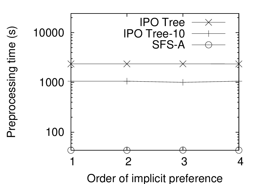
Effect of Order of Implicit Preference: For IPO tree, the number of set operations is given by where is the order of implicit preference. Hence, in Figure 7(b), the query time for IPO Tree increases. The query times for SFS-A and SFS-D are slightly dropping because the skyline size decreases when the order of implicit preference increases. It is obvious that neither the pre-processing or storage will be affected. Figure 7(d) shows that the size of affected skyline points increases. This is because more nominal values involved in the preference affect more data points.
5.2 Real Data Set
To demonstrate the usefulness of our methods, we ran our algorithms on a real data set, Nursery data set, which is publicly available from the UCIrvine Machine Learning Repository22 2 http://kdd.ics.uci.edu/. In this data set, there are 12,960 instances and 8 attributes. The experimental setup is same as [20]. There are six totally-order attributes and two nominal attributes, namely form of the family and the number of children. (Note that although the number of children is a numeric attribute, it is not clear whether a family with one child is “better” than a family with two children.) The cardinality of both nominal attributes are equal to 4. The results in the performance are similar to those for the synthetic data sets. Figure 8 shows the results on the real data set with the effect of the order of implicit preference.
5.3 Main Observations
The major findings from the experiments are the followings. The SFS-D algorithm cannot meet real-time requirements, since the query time is at least in terms of tens of seconds and, in some cases, exceeds 1000 seconds. In general, IPO Tree is the fastest but SFS-A can also return the result within a second in most cases and under 20 seconds in the worst case, and is orders of magnitude faster than SFS-D. The results with IPO Tree-10 show that, by handling a smaller set of nominal values, one can control both the pre-processing and storage costs. A hybrid approach adopting IPO Tree for popular values and SFS-A for handling queries involving the remaining values is a sound solution.
6 Conclusion
Most previous works on the skyline problem consider data sets with attributes following a fixed ordering. However, nominal attributes with dynamic orderings according to different users exist in almost all conceivable real-life applications. In this work, we study the problem of online response for such dynamic preferences, two methods are proposed with different flavors: a semi-materialization method and an adaptive SFS method. Our experiments show how our proposed algorithms are useful in different problem settings.
References
- [1] S. Borzsonyi, D. Kossmann, and K. Stocker. The skyline operator. In ICDE, 2001.
- [2] C. Chan, P.-K. Eng, and K.-L. Tan. Efficient processing of skyline queries with partially-ordered domains. In ICDE, 2005.
- [3] C.-Y. Chan, P.-K. Eng, and K.-L. Tan. Stratified computation of skylines with partially-ordered domains. In SIGMOD, 2005.
- [4] S. Chaudhuri, N. Dalvi, and R. Kaushik. Robust cardinality and cost estimation for skyline operator. In ICDE, 2006.
- [5] J. Chomicki. Database querying under changing preferences. In Annals of Mathematics and Artificial Intelligence, 2006.
- [6] J. Chomicki. Iterative modification and incremental evaluation of preference queries. In FoIKS, 2006.
- [7] J. Chomicki, P. Godfrey, J. Gryz, and D. Liang. Skyline with presorting. In ICDE, 2003.
- [8] J. L. B. et al. Fast linear expected-time algorithms for computing maxima and convex hulls. In SODA’90.
- [9] J. L. B. et al. On the average number of maxima in a set of vectors and applications. In Journal of ACM, 25(4), 1978.
- [10] O. B.-N. et al. On the distribution of the number of admissable points in a vector random sample. In Theory of Probability and its Application, 11(2), 1966.
- [11] W.-T. B. et al. Eliciting matters - controlling skyline sizes by incremental integration of user preferences. In DASFAA’07.
- [12] W.-T. B. et al. Exploiting indifference for customization of partial order skylines. In the 10th International Database Engineering and Applications Symposium, 2006.
- [13] D. Kossmann, F. Ramsak, and S. Rost. Shooting stars in the sky: An online algorithm for skyline queries. In VLDB, 2002.
- [14] D. Papadias, Y. Tao, G. Fu, and B. Seeger. An optimal and progressive algorithm for skyline queries. In SIGMOD, 2003.
- [15] D. Papadias, Y. Tao, G. Fu, and B. Seeger. Progressive skyline computation in database systems. In ACM Transactions on Database Systems, Vol. 30, No. 1, 2005.
- [16] J. Pei, A. W.-C. Fu, X. Lin, and H. Wang. Computing compressed multidimensional skyline cubes efficiently. In ICDE‘07.
- [17] J. Pei, W. Jin, M. Ester, and Y. Tao. Catching the best views of skyline: A semantic approach based on decisive subspaces. In VLDB, 2005.
- [18] J. Pei, Y. Yuan, and X. L. et al. Towards multidimensional subspace skyline analysis. In ACM TODS, 2006.
- [19] K.-L. Tan, P. Eng, and B. Ooi. Efficient progressive skyline computation. In VLDB, 2001.
- [20] R. Wong, J. Pei, A. Fu, and K. Wang. Mining favorable facets. In SIGKDD, 2007.
- [21] R. Wong, J. Pei, A. Fu, and K. Wang. Online skyline analysis with dynamic preferences on nominal attributes. In Technical Report, http://www.cse.cuhk.edu.hk/kdd, 2007.
- [22] T. Xia and D. Zhang. Refreshing the sky: The compressed skycube with efficient support for frequent updates. In SIGMOD, 2006.
- [23] Y. Yuan, X. Lin, Q. Liu, W. Wang, J. X. Yu, and Q. Zhang. Efficient computation of the skyline cube. In VLDB, 2005.
7 Appendix: Proof of Theorem 2
Proof: We need to show that a point is in if and only if it is in . For each direction, we prove by contradiction.
[A] Firstly, assume is in , and suppose that is not in . Then, by Theorem 1, since and is a refinement of , we deduce that . Thus, must satisfy the following:
Condition 1: and
Condition 2: .
Consider Condition 2. Since , there exists a data point dominating w.r.t . In other words, with respect to , for all and in at least one dimension , . Let be the set of dimensions where w.r.t . Besides, for all dimensions other than , the partial orders of and are the same. Hence, w.r.t. , for all . There are two subcases: Case (i): and Case (ii): .
Case (i): . For all , since w.r.t and the partial orders in are those in , we have w.r.t. . Also, w.r.t. , for all . Hence, since , for dimension , it must be the case that w.r.t . Otherwise, is dominated by w.r.t , and cannot be in . Since w.r.t , we have . Since w.r.t. for all , and , we have w.r.t . Since the implicit preference in is “”, we conclude that cannot be . Since is “” and w.r.t , must be in . However, this violates Condition 1 discussed above. Hence, we arrive at a contradiction.
Case (ii): . We obtain w.r.t. . Besides, since the implicit preference in is “”, must be equal to and cannot be equal to . Since , there is no other point including dominating w.r.t. . Note that, w.r.t. , for all . We obtain w.r.t. . (Otherwise, w.r.t and is dominated by w.r.t. , which leads to a contradiction.) Besides, since , and is “”, must be in . However, this violates Condition 1. Hence, we arrive at a contradiction.
[B] Conversely, consider a point in . Suppose that is not in . Thus, is dominated by some point w.r.t. . That is, w.r.t , for all and for at least one dimension .
Since , we know that at least one of the following two conditions holds.
Condition 3: and , or
Condition 4: and .
Consider Condition 3. Since and where is a refinement of , and for all , we deduce that exists in partial orders of but not in partial orders of . Since w.r.t. , and is “”, we deduce . For each possible binary order w.r.t. where and , we also conclude that exists in the partial orders of , which leads to a contradiction.
Consider Condition 4. Since , and differ only at dimension , we only need to check their implicit preferences to see that, whenever (or ) w.r.t. , it is also true w.r.t. or . Therefore, also dominates w.r.t. or . That is, or , which leads to a contradiction.