Scaling and low energy constants in lattice QCD with $N_{\rm f}=2$ maximally twisted Wilson quarks

The values of $\kappa$ in table 1 of Ref. [4] result from implementing maximal twist as discussed here. The formal definition of maximal twist for Wilson quarks reads: $m_{\rm R}=0$ and $\mu_{\rm R}={\rm O}(a^{0})$ for all lattice spacings $a$ as $a\to 0$, with renormalized mass parameters

At the non-perturbative level any legitimate estimate of the critical mass, $m_{\rm crit}$, is affected by terms of O($a\Lambda_{\rm QCD}^{2}$) and O($a\mu\Lambda_{\rm QCD}$), which however do not invalidate the definition of maximal twist. Following Refs. [5, 6], for each $\beta$ (and $\mu$) one can define maximal twist by demanding ¹¹ 1 Here quark bilinears are written in the unphysical quark basis ($\chi$, $\bar{\chi}$) where the Wilson term has its standard form.

at values of $x_{0}$ and $L$ so large that the (charged) one-pion state dominates the correlators on the r.h.s. This prescription fixes the lattice artifact O($a\Lambda_{\rm QCD}^{2}$) in the critical mass in such a way that, provided $\mu\gtrsim a^{2}\Lambda_{\rm QCD}^{3}$, the dominating (relative) cutoff effects left-over in physical observables ²² 2 Concerning the $\pi^{0}$-mass, in Ref. [7] it is argued that the possibly large O($a^{2}$) artifact on this observable is merely due to the large value taken by a (continuum) matrix element present in the Symanzik expansion of all lattice correlators where the $\pi^{0}$ state contributes, rather than to the presence of dimension six operators with large coefficients in the Symanzik effective action. This implies that this cutoff effect represents an exceptional, though important case. are expected to be numerically as small as O($a^{2}\Lambda_{\rm QCD}^{2}$). A detailed analysis [6] shows that such cutoff effects are actually products of (two) terms of order $a\Lambda_{\rm QCD}$, $a\mu$ (negligible for small $\mu$) or $a^{3}\Lambda_{\rm QCD}^{4}\mu^{-1}$ (higher order in $a$, but enhanced for small $\mu$).

In practice, as we are interested in simulations with $\mu\gtrsim\mu_{\rm LOW}$, in order to minimise the work for the tuning of $\kappa$, we choose to impose the condition (2) only for $\mu=\mu_{\rm LOW}$. With this choice, in the region where $\mu<\Lambda_{\rm QCD}$ we expect [6, 1] the numerically dominating cutoff effects on physical observables to be modulated by factors of $\mu_{\rm LOW}/\mu$ as $\mu$ is varied (for instance one can have contributions from terms of order $(a\Lambda_{\rm QCD}\mu_{\rm LOW}/\mu)^{2}$). With $\kappa$ fixed according to the criterion described above, maximal twist is implemented properly, provided

where the coefficient $C$ has to be learned from numerical experiment. In our $N_{\rm f}=2$ setup, $C~\sim~2$ (assuming $\Lambda_{\rm QCD}=250$ MeV) is essentially determined by the condition that MC simulations exhibit no metastabilities (see e.g. Ref. [8], sect. 5.5). At fixed $\mu_{\rm R}$ a smooth approach to the continuum limit is to be expected if maximal twist has been realized at (approximatively) the same value of $\mu_{\rm R\;LOW}$ in physical units for all the considered lattice resolutions.

Our practical implementation of maximal twist is illustrated by Fig. 1a, where we show $m_{\rm R}r_{0}\propto m_{\rm PCAC}$ vs. $\mu_{\rm R}r_{0}\propto\mu$ for $\beta=4.05$, $3.9$ and $3.8$ (use of renormalized quantities eases the comparison). Details on $r_{0}/a$ and $Z_{P}$ (actually $Z_{P}(\overline{\rm MS},2~{\rm GeV})$) are given below.

For $\beta=4.05$ and $3.9$ we could fulfill our criterion for maximal twist at $\mu_{\rm R\;LOW}\simeq 0.047r_{0}^{-1}$ with good statistical precision: as shown in Fig. 1a, $m_{\rm R}/\mu_{\rm R\;LOW}=Z_{A}m_{\rm PCAC}/\mu_{\rm LOW}$ is consistent with zero within the statistical error, that we call $\epsilon/\mu_{\rm LOW}$. As a rule of thumb, we demand $\epsilon/\mu_{\rm LOW}$ to be such that, numerically, $a\Lambda_{\rm QCD}\epsilon/\mu_{\rm LOW}\lesssim 0.01$. Considering the form of the $d=5$ term in the Symanzik effective Lagrangian one finds in fact that $a\Lambda_{\rm QCD}\epsilon/\mu$ is the expected order of magnitude of the unwanted (relative) cutoff effects that may contaminate physical observables if, due to numerical error, $m_{\rm PCAC}(\beta,\mu)$ takes the value $\epsilon Z_{A}^{-1}$, rather than zero. Having no a priori control on the coefficients of this order of magnitude estimate, we can only learn from the numerical experience of a scaling test (involving our statistically most precise observables, i.e. $f_{\rm PS}$ and $m_{\rm PS}$) whether our rule of thumb yields a sufficiently accurate tuning to maximal twist.

At $\beta=3.8$ our implementation of maximal twist was not as precise as wished due to the long-range statistical fluctuations that, for $\mu_{R}\lesssim 0.1r_{0}^{-1}$, were observed in our MC simulations (see Ref. [4] for information on autocorrelation times). These fluctuations, which increase in MC-time length and (weakly) in amplitude as $\mu$ decreases, have a major impact on those observables, such as the plaquette and $am_{\rm PCAC}$, that are not continuous at the Singleton-Sharpe (1^st order) lattice phase transition [8, 9], rendering somewhat problematic the estimate of their statistical errors. This is manifest in Fig. 1a from the two non-coinciding points obtained for the lowest $\mu_{\rm R}$ at $\beta=3.8$, coming from two independent simulations at slightly different $L$ (ensembles A1 and A5 in tab. 1 of Ref. [4]). In this case, the quoted (possibly underestimated) statistical errors are larger than required by our rule of thumb.

In our scaling analyses we employ the Sommer scale $r_{0}$ [10] to eliminate the lattice spacing $a$. This is meant only as an intermediate step. In the end $r_{0}$ will be eliminated in favour of $f_{\pi}$ (i.e. $f_{\rm PS}$ at the physical point) to get the scale for all dimensionful quantities. The value of $r_{0}$ for the various ensembles was obtained with a better than 0.5% accuracy, starting from Wilson loops made out of HYP-smeared temporal links [11] and APE-smeared spatial links. Employing several interpolating operators for static quark-antiquark ($Q\bar{Q}$) states, corresponding to different spatial smearings, leads to a matrix of correlators, from which the (lowest) levels of the potential $V_{Q\bar{Q}}(r)$ are estimated by solving a generalized eigenvalue problem. A fit to the $r$-dependence of the ground state gives $r_{0}(\mu)/a$. For each $\beta$, the latter shows a rather mild $\mu$-dependence, which is well described by a first order polynomial in $\mu^{2}$. The following values, extrapolated to the chiral limit and denoted simply as $r_{0}/a$, will be used in this work (those at $\beta=4.05$ and $\beta=3.8$ must be viewed as preliminary):

$r_{0}/a|_{\beta=4.05}=6.61(3)\,,\quad$ $r_{0}/a|_{\beta=3.9}=5.22(2)\,,\quad$ $r_{0}/a|_{\beta=3.8}=4.46(3)\,.$

Note that a fit by a second order polynomial in $\mu$ gives compatible results. An overview of the results for $r_{0}(\mu)$ for all $\beta$’s is given in Fig. 1b, where the axes are normalized in terms of the appropriate chirally extrapolated $r_{0}$. For $\beta=3.8$ the point at the lowest $\mu$-value (ensemble A1) is preliminary and carries a still poorly estimated statistical error. It was hence not used in the extrapolation to the chiral limit. More details will be given in a forthcoming publication.

In the study of the scaling of the renormalized quark mass $\mu_{R}$ one needs the renormalization constant $Z_{P}(\beta;aq)$ at a common scale $q$ for all the considered values of $\beta$. This renormalization constant, as well as the scale-independent one $Z_{A}(\beta)$, was also employed in Fig. 1a. ⁴⁴ 4 For the renormalization constants we keep the names they are given in the literature for the standard (untwisted) Wilson quark lattice formulation, as obviously their values do not change with respect to the untwisted Wilson case. Preliminary O($a$) improved estimates of the renormalization constants of quark bilinear operators are reported in Ref. [12]. There the results for $Z_{A}$ are rather precise (at the 1.5% level), while the quoted uncertainties on $Z_{P}$ are still substantially larger.

In view of this situation, in our scaling analysis of $\mu_{R}$ we do not use the values of $Z_{P}$ quoted in Ref. [12]. We rather employ the scale- and scheme-independent ratios $Z_{P}(\beta;aq)/Z_{P}(\beta_{\rm ref};a_{\rm ref}q)$, which we extract with a statistical accuracy of $\sim 1\%$ from the relation (exact up to O($a^{2}$) terms)

in order to compare the values of $\mu_{R}(\beta;aq)Z_{P}(\beta_{\rm ref};a_{\rm ref}q)$ at different values of $\beta$ and of the PS-meson mass. In eq. (4), $a\mu(\beta;m_{\rm PS}r_{0}=1;L/r_{0}\simeq 5)$ is the value of $a\mu$ for which, at a given $\beta$ and $L/r_{0}\simeq 5$, one finds $m_{\rm PS}r_{0}=1$. ⁵⁵ 5 This value of $m_{\rm PS}r_{0}$ was chosen so as to lie in the region where errors from interpolation to the reference mass and cutoff effects are smallest. The scaling is obviously not affected by the extra overall factor $Z_{P}(\beta_{\rm ref};a_{\rm ref}q)$, which is removed in the end (in order to give an idea of the values of the renormalized quark masses). In the following we choose $\beta_{\rm ref}=3.9$, where we most reliably know (see Ref. [12]) $Z_{P}(\beta_{\rm ref};a_{\rm ref}q)$, we evaluate for $\beta=4.05$ and $\beta=3.8$ the $Z_{P}$-ratios from eq. (4) and we finally obtain estimates of $\mu_{R}(\beta;aq)$ at $q=2~{\rm GeV}$ in the $\overline{\rm MS}$ scheme for all $\beta$’s. An important drawback of this method is the fact that cutoff effects stemming from data obtained at different $\beta$-values mix up in the quark mass renormalization, which in general may fake the genuine $a$-dependence and cast doubts on the reliability of any continuum extrapolation. Nevertheless, since our data for $\beta=4.05$ and $3.9$ show no statistically significant cutoff effects in the relation of $f_{\rm PS}$ to $m_{\rm PS}^{2}$ and in the values of $\mu_{R}(\beta;aq)Z_{P}(\beta_{\rm ref};a_{\rm ref}q)$, we can obtain an estimate of the continuum limit of $\mu_{R}$ (in units of $r_{0}$) by taking an average of the results at these two $\beta$-values. A similar remark holds for the determination of $\widehat{B}_{0}$ and the chiral condensate in sect. 4. As discussed below, for all observables we associate to our continuum limit estimates a conservative systematic error obtained by comparing them to the corresponding results from data at $\beta=3.8$.

It is well known that matching simulation data obtained at finite $L$ and for $m_{\rm PS}\geq 300$ MeV to the physical pion point requires a delicate analysis. The impact of residual O($a^{2}$) effects (even if small) on such an analysis might be enhanced if the continuum limit is performed as the last step. It is therefore advisable to perform first a continuum limit extrapolation at different (suitably chosen) fixed physical conditions and then use Chiral Perturbation Theory ($\chi$PT) to correct for finite size effects and reach the physical pion point. This is the strategy we follow in sect. 4.1.1, based on the results of the scaling test presented in sect. 3.1. As far as one is concerned with data, such as those at $\beta=4.05$ and $3.9$, where no significant cutoff effects are observed, a conceptually equivalent approach is that of performing a combined analysis of all data by means of continuum $\chi$PT formulae. The outcome of this approach, which is detailed in Ref. [4], is summarised in sect. 4.1.2. For comparison we also discuss in sect. 4.1.3 the results of fits to continuum $\chi$PT formulae where the data corresponding to different lattice spacings are treated separately.

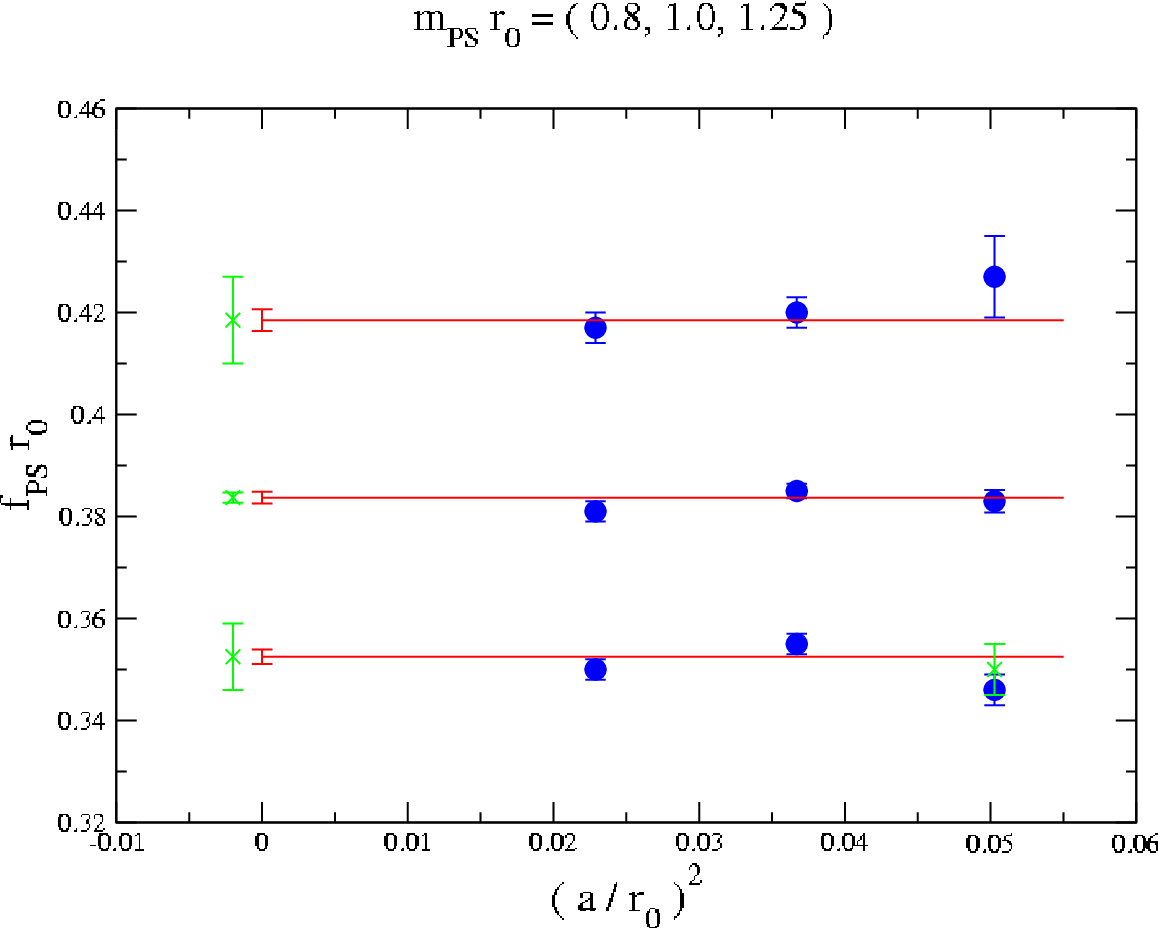
The typical relative statistical errors are (conservatively) estimated to be about 0.7% for $m_{\rm PS}r_{0}$, 1.0% for $f_{\rm PS}r_{0}$ and 1.5% for $\mu_{\rm R}r_{0}$. In the latter case, besides the error on $r_{0}/a$, only the uncertainty (typically about 1.2%) on the $Z_{P}$-ratios (see eq. (4)), is taken into account and hence shown in Fig. 3. The error on $Z_{P}(\beta_{\rm ref};a_{\rm ref}q)$ is omitted here, as it plays no role, while in sect. 4 it is taken into account, as it matters for the final values of $\widehat{B}_{0}$, the chiral condensate and $m_{ud}$.

The condition (i) is immediately fulfilled once all quantities are expressed in units of $r_{0}$. As for the other two conditions, we first implement the condition (iii) by “moving” via resummed $\chi$PT formulae (see Ref. [14]) the data for $f_{\rm PS}$ and $m_{\rm PS}$ from the simulation volume $L^{3}$ to the reference one $L_{\rm ref}^{3}$. As simulations were done with $L\in(2.0,2.4)$ fm, the numerical change in the data is very tiny (never larger than 0.7%) and thus statistically almost irrelevant. Then, in order to match the reference values of $m_{\rm PS}r_{0}$ given in (ii), we perform interpolations (in few cases also short extrapolations) of the values of $f_{\rm PS}r_{0}$ and $\mu r_{0}$. For this purpose we try both (low order) polynomial and $\chi$PT-inspired fits to the data. The spread among the different fits with good $\chi^{2}$, whenever statistically significant, is added linearly to the interpolation error. In this way one ends up with the blue filled circle data points (and errorbars) in the Figs. 2 and 3.

For each value of $m_{\rm PS}r_{0}$ we obtain preliminary estimates of the continuum limit values of $f_{\rm PS}r_{0}$ and $\mu_{\rm R}r_{0}$ by fitting to a constant (red line in the figures) only the data points from simulations at $\beta=4.05$ and $\beta=3.9$. The results, with only statistical error from the continuum extrapolation, are shown in red in Figs. 2 and 3. In all cases the difference between the result of the continuum extrapolation and the central value (blue filled circle point) for $\beta=3.8$ is taken as an estimate of the systematic error (indicated with a green cross placed at a slightly negative value of $a$) on the continuum limit result. Since the latter is obtained by simply taking a weighted average of the results at $\beta=4.05$ and $3.9$, the introduction of such an error appears necessary. Moreover, the quality of the data in the figures suggests that the way we estimate this systematic error is rather conservative. Finally, the green crosses (and errorbars) appearing in Figs. 2 and 3 at $(a/r_{0})^{2}\sim 0.05$ show, whenever the displacement is larger than one standard deviation, where the actual data would move if one were correcting for the leading effect of the numerical error (denoted by $\epsilon$ in sect. 1.1) in imposing $m_{\rm PCAC}=0$. We refer to the results of such a correction (explained in sect. 3.2) as to “data moved to maximal twist”.

The procedure of “moving data to maximal twist” can be seen as a way of testing whether statistical errors in the tuning to maximal twist have any significant impact on the observables of interest. If one has $Z_{A}m_{\rm PCAC}=\epsilon$ (rather than zero), the effective twist angle in the Symanzik Lagrangian is $\alpha=\pi/2-\theta$ with $\tan\theta=m_{R}/\mu_{R}=\epsilon/\mu$. Treating $\epsilon$ as an O($a^{0}$) quantity and neglecting O($a\theta$) and O($a^{2}$) effects, the consequences of a deviation from maximal twist are in general twofold. First, the effective renormalized quark mass becomes $M_{R}=(\mu_{R}^{2}+m_{R}^{2})^{1/2}=\mu_{R}/cos\theta$. Second, in all operator matrix elements any operator formally non-invariant under axial-$\tau^{3}$ transformations must be reinterpreted consistently with the twist angle being $\alpha=\pi/2-\theta$ (rather than $\pi/2$). As a consequence, once the hadronic states of interest are correctly identified, simple $\theta$-dependent formulae can be derived that allow to extract properly the matrix elements of operators non-invariant under axial-$\tau^{3}$ transformations. For instance, the (renormalized) operator $Z_{V}\bar{\chi}\gamma_{\mu}\tau^{2}\chi$ (written in the basis where the Wilson term has its standard form) coincides with $\cos\theta A_{\mu\;R}^{1}+\sin\theta V_{\mu\;R}^{2}$, where $A_{\mu\;R}^{1}$ ($V_{\mu\;R}^{2}$) is the physical axial (vector) current. Consequently one finds $\;\;<\pi^{1}|Z_{V}\bar{\chi}\gamma_{\mu}\tau^{2}\chi|\Omega>|_{m_{R},\mu_{R}}\;=\;\cos\theta<\pi^{1}|A_{\mu\;R}^{1}|\Omega>|_{M_{R}}+{\rm O}(a\theta,a^{2})\;$, which implies $\;m_{\rm PS}f_{\rm PS}|_{M_{R}}=<\pi^{1}|Z_{V}\bar{\chi}\gamma_{0}\tau^{2}\chi|\Omega>|_{m_{R},\mu_{R}}/\cos\theta+{\rm O}(a\theta,a^{2})$.

From these arguments it follows that $m_{\rm PS}$-data need not be moved, while the data for $\mu_{\rm R}$ and $f_{\rm PS}$ are “moved to maximal twist”, up to ${\rm O}(a\theta,a^{2})$, by dividing them by $\cos\theta$, where $\theta$ is obtained from the (interpolated) actual values of $\epsilon$ and $\mu$ in our data sets. It turns out that the change implied by this correction is larger than one standard deviation (of the uncorrected data) only for the two smallest reference values of $m_{\rm PS}r_{0}$ at $\beta=3.8$. After such correction all the data points at $\beta=3.8$ (including the two most chiral ones) fit very nicely into the scaling picture suggested from the corresponding data at $\beta=3.9$ and $\beta=4.05$.

However, any data where the above correction was statistically relevant can be hardly used for a continuum extrapolation, because the residual (uncorrected) O($a\theta$) lattice artifacts depend on the details of the numerical errors at the different $\beta$-values and hence need not to scale as $a\to 0$. Nevertheless, at a more qualitative level, the procedure of “moving data to maximal twist” confirms that, even at $\beta=3.8$ (i.e. $a\simeq 0.1$ fm), the lattice artifacts in the charged PS-meson sector appear to be quite small, provided maximal twist is implemented precisely, e.g. according to the criteria of sect. 1.1. In fact such a precise implementation is rather hard to achieve in the case of our simulations at $\beta=3.8$, as we found $\tau_{\rm int}(am_{\rm PCAC})={\rm O}(100)$, see sect. 1.1 and Ref. [4].

As anticipated in sect. 2.2, given the good scaling behaviour of our data, we present preliminary continuum estimates of LEC and $m_{ud}$ that stem from two analyses – see sects. 4.1.1 and 4.1.2. In sect. 4.1.3 we give the corresponding results that are obtained at two fixed lattice spacings, $a(\beta=4.05)$ and $a(\beta=3.9)$. The latter results will serve mainly for estimating (in the way detailed below) the systematic error due to residual O($a^{2}$) cutoff effects.

Concerning other systematic errors, we note: (i) residual uncertainties in the CDH-formulae for FS effects are small, compared to other systematic errors – see the discussion in Ref. [4]; (ii) the possible impact of NNLO corrections to the formulae (5)–(6) for the quark mass dependence is minimized by taking out of the analyses the points with highest values of $m_{\rm PS}$ (we checked that fits are stable if we leave out data with $m_{\rm PS}>500$ MeV – more details in a forthcoming publication).

Our preliminary results in the $\overline{\rm MS}$-scheme at scale $q=2$ GeV are obtained using the RI-MOM estimate [12] of $Z_{P}$ at $\beta=3.9$ (converted to $\overline{\rm MS}$ by using NNNLO perturbation theory) and the $Z_{P}$-ratios from the analysis of sect. 4.1.2 (combined fit) or 4.1.1 (fit in the continuum). The average light quark mass $m_{ud}({\overline{\mbox{\rm MS}}},2{\rm GeV})$ from the fit in the continuum reads $m_{ud}=3.43(9)(23)\,\textrm{MeV}$. From the combined fit we get $m_{ud}=3.62(10)(23)$ MeV (using all the ensembles) and $m_{ud}=3.49(13)(23)$ MeV (when excluding ensembles $B_{6}$ and $C_{5}$, i.e. with the same set of ensembles as for the fit in the continuum). When considering data at $\beta=3.9$ only (as in sect. 4.1.3), we obtain $m_{ud}=3.62(13)(23)$ MeV. This value is compatible with the one coming from the partially quenched analysis of Ref. [17], $m_{ud}=3.85(12)(40)\,\textrm{MeV}$.

The chiral quark condensate is obtained through $\langle\bar{q}q\rangle({\overline{\mbox{\rm MS}}},2{\rm GeV})=-(1/2)f_{0}^{2}\widehat{B}_{0}({\overline{\mbox{\rm MS}}},2{\rm GeV})$. From the fit after the continuum extrapolation we get $|\langle\bar{q}q\rangle|^{1/3}=272(4)(7)\,\textrm{MeV}$, while from the combined fit analysis we obtain $|\langle\bar{q}q\rangle|^{1/3}=267(4)(7)\,\textrm{MeV}$ (and $|\langle\bar{q}q\rangle|^{1/3}=270(4)(7)\,\textrm{MeV}$ when the ensembles $B_{6}$ and $C_{5}$ are not used). These results are in agreement with an independent estimate at $\beta=3.9$ from the $\epsilon$ regime – see Ref. [18].

In Fig. 5, we show our data (in units of $r_{0}$) for the vector meson “mass”, $\widetilde{m}_{\rm V}$, and the nucleon mass, $m_{\rm N}$, as a function of $m_{\rm PS}^{2}$. For the former one (see Ref. [19] for more details), the scaling appears to be good, although within statistical errors that become of few percents when $m_{\rm PS}\sim 300\div 350$ MeV. In this case, we remark that what we call the “mass” may differ from the actual vector meson mass (the one that becomes $m_{\rho}$ as $m_{\rm PS}\to m_{\pi}$), owing to the effect of virtual $\rho$–$\pi\pi$ mixing. ⁹⁹ 9 The correction is estimated [19] to be almost irrelevant within our present statistical errors: at our most chiral point, where $m_{\rm PS}\sim 300$ MeV, it amounts to $\widetilde{m}_{\rm V}-m_{\rm V}\sim 0.05m_{\rm V}$. Due to the finite volume, the decay of the $\rho$-meson (at rest) into real $\pi\pi$ states is instead forbidden, even when $2m_{\rm PS}<m_{\rm V}$ (which roughly speaking happens in the region $(m_{\rm PS}r_{0})^{2}\lesssim 1$). The data for the nucleon mass are also preliminary (see Ref. [20]): at $\beta=4.05$ only two data points are available, which however appear to agree quite well with the data points at $\beta=3.9$.

To compute charmed observables we adopt a partially quenched (PQ) setup, which is detailed in Ref. [21]. ¹⁰¹⁰ 10 The proof of automatic O($a$) improvement given in Ref. [22] for a fully unquenched mixed action framework goes through also in the PQ mixed action setup of Ref. [21], where the quark masses of the valence $s$ and $c$ quarks are taken finite and hence different from those (infinite in the present case) of the corresponding sea quarks. With the notation of Ref. [22] for valence quarks, the correlators for $D$ ($\bar{c}d$) and $D_{s}$ ($\bar{c}s$) charged mesons are computed with Wilson parameters $r_{d}=r_{s}=-r_{c}=1$, in order to have the same nice parametric scaling properties as in the charged pion sector. For the present considerations about scaling we choose close-to-realistic renormalization conditions: $m_{\rm PS}r_{0}=0.7092$ and $\mu_{\tilde{s}}/\mu_{\tilde{c}}=0.082$ (instead of the realistic conditions $m_{\pi}r_{0}\simeq 0.30$ and $\mu_{s}/\mu_{c}\simeq 0.088$). In Figs. 6, $m_{\rm D}$ varies with $\mu_{\tilde{c}}$ at fixed values of $\mu_{\tilde{s}}/\mu_{\tilde{c}}$ and $m_{\rm PS}r_{0}$ (i.e. $\mu_{ud}$). The expected size of the dominating cutoff effects is $(a\mu_{\tilde{c}})^{2}\sim 0.1$, since typically, $a\mu_{\tilde{s}}\in[0.020,\,0.033]$ and $a\mu_{\tilde{c}}\in[0.25,\,0.40]$.

By comparing the preliminary results from $\beta=4.05$ and $\beta=3.9$, we see that the observed scaling violations are not large: from 1–2% (hardly visible within statistical errors) for $f_{\rm D}$ and $m_{\rm D_{s}}$ to 7–8% for $f_{\rm D_{s}}$. Data from a third lattice spacing, $\beta=3.8$, are currently being analysed and may allow for an estimate of continuum limit results.

References

- [1] ETM Collaboration, Ph. Boucaud et al., Phys. Lett. B650, 304 (2007), [hep-lat/0701012].
- [2] C. Urbach, K. Jansen, A. Shindler and U. Wenger, Comput. Phys. Commun. 174, 87 (2006), [hep-lat/0506011].
- [3] R. Frezzotti and G.C. Rossi, JHEP 0408, 007 (2004), [hep-lat/0306014].
- [4] ETM Collaboration, C. Urbach, PoS(LATTICE 2007)022 [arXiv:0710.1517].
- [5] S.R. Sharpe and J.M.S. Wu, Phys. Rev. D71 (2005) 074501, [hep-lat/0411021].
- [6] R. Frezzotti, G. Martinelli, M. Papinutto and G.C. Rossi, JHEP 0604 038 (2006), [hep-lat/0503034].
- [7] ETM Collaboration, R. Frezzotti and G.C. Rossi, PoS(LATTICE 2007)277.
- [8] A. Shindler, arXiv:0707.4093 [hep-lat].
- [9] S. R. Sharpe, Phys. Rev. D 72 (2005) 074510, [hep-lat/0509009].
- [10] R. Sommer, Nucl. Phys. B 411 (1994) 839 [arXiv:hep-lat/9310022].
- [11] M. Della Morte, A. Shindler and R. Sommer, JHEP 0508 (2005) 051, [hep-lat/0506008].
- [12] ETM Collaboration, P. Dimopoulos et al., PoS(LATTICE 2007)241 [arXiv:0710.0975].
- [13] J. Gasser and H. Leutwyler, Phys. Lett. B184, 83 (1987).
- [14] G. Colangelo, S. Dürr and C. Haefeli, Nucl. Phys. B721, 136 (2005), [hep-lat/0503014].
- [15] H. Leutwyler, arXiv:0706.3138 [hep-ph].
- [16] S. Necco, PoS(LATTICE 2007)021.
- [17] ETM Collaboration, B. Blossier et al., [arXiv:0709.4574]; C. Tarantino et al., PoS(LATTICE 2007)374 [arXiv:0710.0329].
- [18] ETM Collaboration, A. Shindler et al., PoS(LATTICE 2007)084.
- [19] ETM Collaboration, C. Michael and C. Urbach, PoS(LATTICE 2007)122 [arXiv:0709.4564].
- [20] ETM Collaboration, C. Alexandrou et al., PoS(LATTICE 2007)087 [arXiv:0710.1173].
- [21] ETM Collaboration, B. Blossier et al., PoS(LATTICE 2007)346 [arXiv:0710.1414].
- [22] R. Frezzotti and G.C. Rossi, JHEP 0410 (2004) 070, [hep-lat/0407002].